Non-Gaussian buoyancy statistics in fingering convection

Abstract

We examine the statistics of active scalar fluctuations in high-Rayleigh number fingering convection with high-resolution three-dimensional numerical experiments. The one-point distribution of buoyancy fluctuations is found to present significantly non-Gaussian tails. A modified theory based on an original approach by Yakhot (1989) is used to model the active scalar distributions as a function of the conditional expectation values of scalar dissipation and fluxes in the flow. Simple models for these two quantities highlight the role of blob-like coherent structures for scalar statistics in fingering convection.

1 Introduction

Fingering convection is a peculiar convective flow, characterized by a counter-gradient density transport, which is of interest for a wide range of fields, including stellar physics, metallurgy and volcanologyTurner74 [1]. It raises particular interest in oceanographySchmitt94 [2, 3], where warm, salty, and light waters floating above fresher, colder and denser waters create finger-favorable conditions. This situation is commonplace in the thermocline of subtropical oceans, where finger-generated diapycnal mixing is believed to affect the meridional overturning circulation, and the uptake of heat and carbon dioxide Schmitt05 [4]. Fingering convection occurs when two buoyancy-changing scalars with different diffusivities are stratified in such a way that the least-diffusing one, if taken alone, would produce an upward, unstable density gradient, but the most-diffusing one reverses this tendency and produces a net downward density gradient. This set-up allows for a doubly-diffusive instability, where infinitesimal perturbations to the initial stratification may undergo exponential growth. If a fluid parcel is displaced downward it looses the stabilizing, most-diffusing scalar at a faster rate than the destabilizing, least-diffusing one, because of the difference in diffusivities. This results in an increase of the density of the parcel, which sinks at a lower depth, where it loses even more stabilizing scalar. A symmetrical argument holds for a fluid parcel displaced upward. While the two scalars are transported along their gradients, a net counter-gradient buoyancy flux results from this mechanism. In the linear theory maximum growth rate is attained at horizontal wavelengths sufficiently small so that the difference in diffusivity of the two scalars is important, but not so small that the damping effect of viscosity becomes dominant (a few centimeters in the oceans), and at a vertical wavelength corresponding to the vertical domain extension Baines&Gill69 [5, 6]. In the fully nonlinear regime, the elongated, finger-like columns of the linear theory break down into shorter plumes, or blobs, as we shall call them, of rising and sinking fluid, having an aspect ratio much closer to one. Vigorous convection arises, dominated by the complicated dynamics of the interacting blobs Merryfield00 [7, 8]. In some instances a secondary instability disrupts the linear profiles of horizontally averaged temperature and salinity, leading to the formation of the so-called “staircases” where finger zones are alternated with slabs of vertically well-mixed fluid Schmitt94 [2, 9].

While ample literature has been devoted to convection problems with a single scalar, the Rayleigh-Bénard set-up being the leading example, convection with two active scalars, such as fingering convection, has yet to be explored to the same extent. In particular, knowledge on the statistical properties of scalar fluctuations can be useful for constraining and testing models of the convective scalar fluxes. In this paper we use high-resolution three-dimensional numerical simulations to explore the high-Rayleigh number regime of fingering convection and we analyze and interpret the scalar fluctuation distributions in these flows using a novel formulation of a classical theoretical approach.

2 The Simulations

2.1 The equations of fingering convection

As customary in this problem, we denote the least-diffusing scalar as salinity, $S$, and the most-diffusing one as temperature, $T$, even if the actual physical nature of the two scalars may be different. We consider a fluid layer of thickness $d$ confined above and below by perfectly conducting, parallel, plane plates mantained at constant temperature and salinity. We bring the problem to a non-dimensional form by scaling temperatures and salinity with their plate differences $\Delta T$ and $\Delta S$, scaling lengths with the layer thickness, $d$, and using the haline diffusive time, $\tau_{S}=d^{2}/\kappa_{S}$, as a timescale, with $\kappa_{S}$ the haline diffusivity. The control parameters of the problem are the Prandtl, Lewis, thermal and haline Rayleigh numbers, defined as

$$Pr=\frac{\nu}{\kappa_{T}},\,Le=\frac{\kappa_{T}}{\kappa_{S}},\,R_{T}=\frac{g\alpha\Delta T\,d^{3}}{\nu\kappa_{T}},\,R_{S}=\frac{g\beta\Delta S\,d^{3}}{\nu\kappa_{S}},$$

respectively. In these expressions $\nu$ is the kinematic viscosity, $\kappa_{T}$ is the thermal diffusivity, $g$ is the modulus of the gravity acceleration and $\alpha$ and $\beta$ are the thermal and haline linear expansion coefficients. From these the density ratio $R_{\rho}=Le\,R_{T}/R_{S}$ can be defined. Linear stability analysis shows that a necessary condition for fingering instability is $1<R_{\rho}<Le.$ The density ratio controls directly the intensity of convection in the flow. Values close to one lead to fast instability and violent convection. The haline diffusive time is the longest time scale in this problem. Far from marginality, it is often more convenient to use the convective time scale $\tau_{c}=(Pr\,Le\,R_{S})^{-1/2}\tau_{S}$.

In the Boussinesq approximation, the resulting non-dimensional equations for fingering convection are:

$$\frac{\partial\mathbf{u}}{\partial t}+\mathbf{u}\cdot\nabla\mathbf{u} = -\nabla p+Pr\,Le\left[R_{S}B\,\hat{\mathbf{z}}+\nabla^{2}\mathbf{u}\right],$$ (1)

$$\frac{\partial T}{\partial t}+\mathbf{u}\cdot\nabla T = Le\,\nabla^{2}T,$$ (2)

$$\frac{\partial S}{\partial t}+\mathbf{u}\cdot\nabla S = \hphantom{Le\,}\nabla^{2}S,$$ (3)

$$\nabla\cdot\mathbf{u} = 0,$$ (4)

where $\mathbf{u}=(u,v,w)$ is the solenoidal velocity field of the fluid, $p$ is the pressure, and we have defined the buoyancy field $B=R_{\rho}T-S$. The latter is the dynamically important linear combination of the $T,$ $S$ scalar fields as it appears in the forcing term of the momentum equation (1). Notice that the equations could be rewritten entirely in terms of buoyancy together with some other linear combination of temperature and salinity. In this case buoyancy would play the role of the active, momentum-generating scalar, and the other scalar could be considered almost passive, interacting only with buoyancy through a diffusive term. For example in the oceanographic literature a quantity called “spice” is sometimes defined Flament02 [10] as the linear combination of temperature and salinity which is maximally independent of buoyancy.

We integrate the equations numerically with a code which is pseudospectral in the horizontal directions and with finite differences in the vertical, with a non-homogeneous vertical grid in order to better resolve the boundary layers and with a third-order fractional step method for time advancement Passoni02 [14, 15, 16]. Free slip boundary conditions are used at the top and at the bottom and a laterally periodic domain is assumed.

While the density ratio represents the main control parameter in this type of flows, in the sense that small variations of $R_{\rho}$ determine large variations in the fluxes, we study the changes in the flow determined by changes in the vertical extent of the domain, as encoded in the Rayleigh numbers. It has been suggested that simulations in a vertically periodic domain should yield results comparable with those that could be observed in a physical situation where the vertical extension is many orders of magnitude larger than the scale of the fingers (e.g. Merryfield00 [7, 8]). However, recent work Calzavarini06 [17] casts shadows on the meaningfulness of investigations in such a domain. This requires treating the magnitude of the Rayleigh numbers, and not only their ratio, as an independent free control parameter of the problem. Accordingly here we use a configuration confined between upper and lower rigid plates, and push up the Rayleigh numbers while maintaining a fixed density ratio $R_{\rho}=1.2$, which is sufficient to guarantee vigorous convection. We perform a series of numerical experiments, fixing $Pr=10,Le=3$, and exploring the range $R_{S}=10^{8}-10^{11}$. The vertical domain extension is $-0.5<z<0.5$. The vertical resolution ranges between $N_{z}=145$ (at $R_{S}=10^{8}$) and $N_{z}=809$ layers (at $R_{S}=10^{11}$). The horizontal resolution is maintained at $N_{x}=192$ grid points, while the lateral domain size is scaled in order to be approximately proportional to the horizontal linear instability scale Stern75 [6], according to $L=(R_{S}/10^{9})^{-1/4}$.

2.2 Statistics of scalar fluctuations

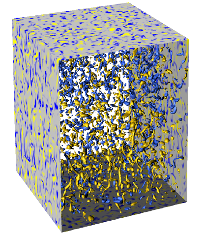
Figure 1: Rendering of buoyancy fluctuation iso-surfaces at the level $2.5\sigma_{B}$, once statistical stationarity has been reached, in the center of the domain between $z=-0.2$ and $z=0.2$. The lateral panels show sections through the flow with a colormap saturating at $3\sigma_{B}$. Yellow(blue) corresponds to positive(negative) buoyancy fluctuations.

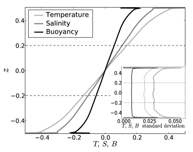
Figure 2: Horizontally and time averaged scalar profiles for the simulation at $R_{S}=10^{11}$; (in the inset) profiles of the standard deviation of scalar fluctuations at fixed $z$. The time averages extend over one hundred convective time units.

Fig. 1 shows an isosurface rendering of the buoyancy fluctuation field for the simulation at $R_{S}=10^{11}$, in the center of the domain, after the solution has reached statistical stationarity. The flow is characterized by the presence of well defined buoyancy structures which transport a large fraction of the vertical buoyancy fluxes and lead to the vertical homogenization of the statistical properties of the flow. Fig. 2 shows vertical profiles of horizontal averages of buoyancy, temperature and salinity, and of the variance of fluctuations respect to these profiles. Note the inverse boundary layers of buoyancy, which testify of a counter-gradient advective transport. An ample central region characterized by a uniform linear background and approximately $z-$independent variance is evident. This is the region of interest for many geophysical applications of fingering convection, including oceanographic problems, all characterized by high Rayleigh numbers and reduced influence of the vertical boundary conditions. Increasing the Rayleigh numbers in our simulations leads to a growth of the height of this central region. The presence of a vertical average background gradient of the scalars is characteristic of fingering convection, and it is consistent with laboratory experiments and observations (e.g Schmitt94 [2, 9]) where approximately uniform vertical mean gradients are reported within the fingers zones.

In the central region buoyancy fluctuations (respect to horizontally averaged buoyancy), vertical velocities, and convective fluxes all vary according to approximate power laws with the Rayleigh number, as summarized in table 1. The table also reports two independent estimates of the characteristic scales of the structures in the buoyancy field: $l_{x}$ is the position of the first zero of the spatial autocorrelation function of buoyancy, computed keeping constant the coordinates $y$ and $z$; $l_{v}$ is the cubic root of the average volume of the connected regions with $|B^{\prime}|\geq 2\sigma_{B^{\prime}}$. Both estimates give similar results.

$R_{S}$	$\sigma_{B^{\prime}}$	$\sigma_{W}$	$\langle WB^{\prime}\rangle$	$l_{x}$	$l_{v}$	$Re$
$10^{8}$	0.0159	432.2	5.81	0.0402	0.0447	0.58
$10^{9}$	0.0132	1017.6	11.06	0.0218	0.0243	0.74
$10^{10}$	0.0099	2621.0	19.45	0.0128	0.0138	1.12
$10^{11}$	0.0078	6271.5	33.56	0.0076	0.0070	1.59
Exponent:	-0.11	0.39	0.25	-0.24	-0.26

Table 1: Statistics of buoyancy fluctuations as a function of haline Rayleigh number, computed at the center of the domain ($-0.2\leq z\leq 0.2$), once statistical stationarity has been reached. The standard deviations of buoyancy fluctuations and of vertical velocities, $\sigma_{B^{\prime}}$ and $\sigma_{W}$, and the vertical convective fluxes, $\langle{WB^{\prime}}\rangle$, are reported; $l_{x}$ and $l_{v}$ are two independent estimates of the size of the structures in the buoyancy field (see text for details). The rightmost column reports the Reynolds number of the buoyancy structures estimated as $Re=\sigma_{W}l_{x}/(LePr)$. The bottom row reports exponents obtained fitting a power law scaling respect to $R_{S}$.

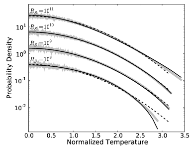
a) b)
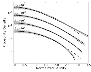
c)

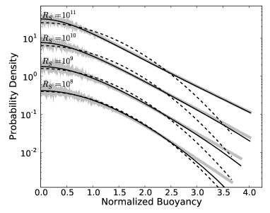
Figure 3: $(a,b,c)$ Probability density functions of the temperature, salinity and buoyancy fluctuations respectively, normalized to unitary variance. Data for four different simulations at $R_{S}=10^{8},10^{9},10^{10},10^{11}$ are reported, gathered over a time interval of one hundred convective times, once stationarity has been reached. For clarity the latter three curves are multiplied by two, four and eight units, respectively. Superimposed on the numerical data are expression (7) and its analogues for temperature and salinity, evaluated using the fits (8) (for temperature and salinity), (9) (for buoyancy) and $E(\mathcal{F}|X)/X=X$. Gaussian distributions with unitary variance are reported for reference, using dashed lines.

Figs. 3(a-c) compare the one-point probability distributions of temperature, salinity and buoyancy fluctuations, for haline Rayleigh numbers $R_{S}=10^{8},10^{9},10^{10},10^{11}$, computed at the center of the domain, $-0.2\leq z\leq 0.2$, once statistical stationarity has been reached. Temperature and salinity present sub-Gaussian distributions at low $R_{S}$, which become roughly Gaussian at intermediate $R_{S}$ and develop tails longer than Gaussian only at the highest $R_{S}$ explored in this work. The distribution of buoyancy, instead, shows non-Gaussian tails already at the lowest $R_{S}$ considered, which become very similar to exponentials at high $R_{S}$.

The emergence of exponential tails in the active scalar distribution is reminiscent of the classical transition to so-called “hard turbulence” for thermal convection, first reported in Castaing89 [18]. In that case buoyancy is determined by only one scalar (temperature), which develops well defined exponential tails at high Rayleigh number. The behaviour of a passive scalar in homogeneous turbulence has been discussed in e.g. in Sinai&Yakhot89 [11, 12] and also in that case non-Gaussian behavior is found. The present case is only partially similar to those just mentioned: no scalar is completely passive in fingering convection, and the buoyant structures have a very different origin and morphology compared to single-scalar convection (finger-like blobs vs. turbulent plumes).

3 A model for the fluctuation distributions

3.1 Yakhot’s approach

The scalar probability distributions described above can be interpreted by adapting to the present case with two active scalars the theory developed by YakhotYakhot89 [13] for the case of high-Rayleigh number thermal convection. An important pre-requisite of that theory is a constant, non-zero vertical gradient of the horizontally averaged density field, a situation which does not occur in the bulk flow of Rayleigh-Bénard convection, but whose presence is, as we have discussed above, the hallmark of fingering convection.

In order to proceed along these lines we express the buoyancy field as $B(x,y,z,t)=B^{\prime}(x,y,z,t)+G_{B}z$, where $G_{B}$ is the vertical gradient of the horizontally averaged buoyancy, and $B^{\prime}$ is the buoyancy fluctuation. The quantities $T^{\prime}$, $S^{\prime}$, $G_{T}$ or $G_{S}$ can be defined analogously. Combining Eq. (2) and (3) we obtain an evolution equation for the buoyancy fluctuation, written in terms of buoyancy and temperature:

$$\frac{\partial B^{\prime}}{\partial t}+\mathbf{u}\cdot\nabla B^{\prime}-wG_{B}=R_{\rho}\left(Le-1\right)\nabla^{2}T^{\prime}+\nabla^{2}B^{\prime}.$$ (5)

We multiply this expression by $B^{\prime 2n-1}$ and denote with $\left\langle\cdot\right\rangle$ a time and volume average. The volume averages are carried over a central portion of the domain, where the assumption of constant gradients holds (represented by the dashed lines of Fig. 2 for our simulations). Assuming a statistically steady state we can integrate by parts; the lateral boundary terms are zero for periodic (or no flux) boundary conditions; the top and bottom terms cancel each other because statitical stationarity implies that the vertical flux of all moments of $B^{\prime}$ must be the same at all heights. Dividing the resulting equation for a generic $n$ by the equation for $n=1$ we obtain

$$(2n-1)\left\langle X_{B}^{2n-2}\chi_{B}\right\rangle=\left\langle X_{B}^{2n-2}\mathcal{F}_{B}\right\rangle,$$ (6)

where we have defined the normalized buoyancy fluctuation, $X_{B}=B^{\prime}/\left\langle B^{\prime 2}\right\rangle^{1/2}$, the normalized buoyancy flux, $\mathcal{F}_{B}=wB^{\prime}/\left\langle wB^{\prime}\right\rangle$ and the normalized buoyancy dissipation rate, $\chi_{B}=\frac{\nabla B^{\prime}\cdot\left[R_{\rho}\left(Le-1\right)\nabla T^{\prime}+\nabla B^{\prime}\right]}{\left\langle\nabla B^{\prime}\cdot\left[R_{\rho}\left(Le-1\right)\nabla T^{\prime}+\nabla B^{\prime}\right]\right\rangle}$. We refer to the latter quantity as ’buoyancy dissipation’, even if it may be negative somewhere in the fluid. In fact, the signature of doubly-diffusive convection is the ability of the second-order derivative terms in the equations to behave as sources of buoyancy fluctuations, rather than solely as sinks. But the large-scale, average effect of these terms remains that of sinks of variance: for $n=1$ Eq. (6) is the balance between the advective rate of extraction of buoyancy variance from the vertical gradients, and its diffusive dissipation rate at small scales. Note that this process cannot be described solely in terms of buoyancy: temperature or salinity fluctuations must appear explicitly in the buoyancy variance dissipation rate.

In the following we interpret the quantities $X_{B},$ $\mathcal{F}_{B},$ and $\chi_{B}$ as stochastic variables and we make our last assumption, namely the equivalence of space-time and ensemble averages. We observe that the probability density of $X_{B}$ must have a compact support, because Eqs. (2) and (3) satisfy a maximum principle, and this forbids arbitrarily large buoyancy fluctuations; therefore the averages that appear in Eq. (6) exist for any integer $n>0$.

From Eq. (6) it is possible to follow Yakhot’s analysisYakhot89 [13] slavishly, obtaining an explicit expression for the probability density of $X_{B}$:

$$P(X_{B})=\frac{E(\chi_{B}|0)P(0)}{E(\chi_{B}|X_{B})}\exp\left[-\int_{0}^{X_{B}}\frac{E(\mathcal{F}_{B}|x)}{xE(\chi_{B}|x)}\,dx\right],$$ (7)

where $E(\cdot|\cdot)$ denotes a conditional average. This is an exact relationship for the one-point probability density of buoyancy fluctuations which depends only on two unknown functions, namely the expected values of the buoyancy fluxes, $E(\mathcal{F}_{B}|X_{B})$, and of the dissipation, $E(\mathcal{\chi}_{B}|X_{B})$, conditioned on the buoyancy fluctuations. The constant $P(0)$ is fixed by the normalization requirement of the density function. Far from the physical boundaries it is reasonable to assume that the actual solution of the Boussinesq equations (1-4) will have the same up-down simmetry of the equations themselves: It follows that $P(X_{B})$, and the unknown conditional expectations $E(\chi_{B}|X_{B})$ and $E(\mathcal{F}_{B}|X_{B})$, are even functions of $X_{B}$. Furthermore, $E(\mathcal{F}_{B}|0)=0$, because $\mathcal{F}_{B}=0$ where $X_{B}=0$.

Theoretical expressions for the distributions of normalized temperature and salinity fluctuations, or of their linear combinations, such as spice, can be obtained following the same approach. This yields expressions which are functionally identical to Eq. (7), but where (e.g. for temperature) the quantities $X_{T}=T^{\prime}/\left\langle T^{\prime 2}\right\rangle^{1/2}$, $\mathcal{F}_{T}=wT^{\prime}/\left\langle wT^{\prime}\right\rangle$, $\chi_{T}=|\nabla T^{\prime}|^{2}/\left\langle|\nabla T^{\prime}|^{2}\right\rangle$ appear in place of $X_{B}$, $\mathcal{F}_{B}$, $\chi_{B}$. In the following we will also use the unlabeled symbols $X$, $\mathcal{F}$, $\chi$ for, respectively, normalized fluctuations, fluxes and dissipation of a generic scalar.

3.2 Scalar fluxes

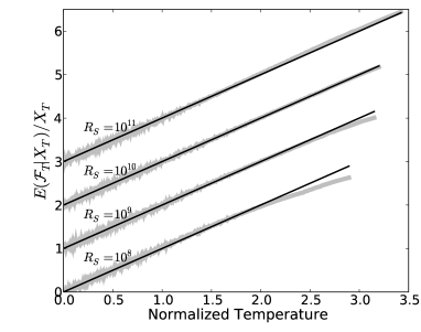
a) b)
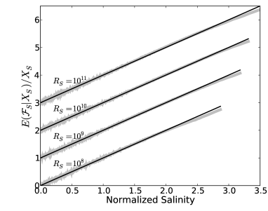
c)

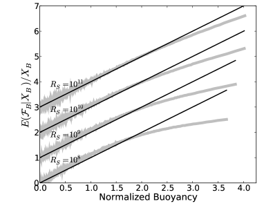
Figure 4: $(a)$ Plot of $E(\mathcal{F}_{T}|X_{T})/X_{T}$ vs. $X_{T}$ for the four simulations at $R_{S}=10^{8},10^{9},10^{10},10^{11}$; data are gathered for one hundred convective times, once statistical stationarity has been reached. For clarity the latter three curves are shifted upward by one, two and three units, respectively. The straight lines are the theoretical fit $E(\mathcal{F}|X)/X=X$. Only the positive normalized fluctuation half-plane is shown. For the negative half-plane odd symmetry holds. $(b,c)$ The analogous plots for salinity and buoyancy.

The normalized, conditional, averages of the temperature and salinity fluxes in our numerical experiments, $E(\mathcal{F}_{T}|X_{T})/X_{T}$ and $E(\mathcal{F}_{S}|X_{S})/X_{S}$, are reported in Figs. 4(a,b), computed in the positive half-plane. The linear expression $E(\mathcal{F}|X)/X=X$ fits very well the data, particularly at larger Rayleigh numbers. Small deviations from linearity are evident only for large temperature or salinity fluctuations. Note that no further constants appear in this expression due to the identity $\langle\mathcal{F}\rangle=\int{E(\mathcal{F}|X)P(X)dX}$ and the requirements $\langle X^{2}\rangle=1$ and $\langle\mathcal{F}\rangle=1$. This result has a very simple interpretation in the flow under study, if temperature and salinity are considered as almost passive scalars: as a parcel of fluid moves downward (upward) in the presence of background gradients, it carries with it the temperature and salinity values corresponding to a higher (lower) level, thus generating positive (negative) temperature and salinity fluctuations. Molecular diffusion tends to remove the fluctuation, until an equilibrium between these two competitive factors is found, leading to a fluctuation proportional to the vertical speed of the parcel of fluid. From this, the relationship $E(\mathcal{F}|X)/X=X$ trivially follows.

A different mechanism must apply for buoyancy fluctuations, which play a direct role in determining vertical accelerations in the flow and which are generated by the doubly-diffusive mechanism, rather than by vertical displacement of the fluid. Fig. 4(c) reports the normalized conditional averages of buoyancy fluxes, $E(\mathcal{F}_{B}|X_{B})/X_{B}$. While the linear expression $E(\mathcal{F}_{B}|X_{B})/X_{B}=X_{B}$ again fits the data, more severe deviations from linearity are evident at large buoyancy values, particularly at low Rayleigh numbers. This result is consistent with a scenario where the advective fluxes are determined to a large extent by the motion of blobs of buoyancy of characteristic size $l$, travelling, on average, at a vertical velocity $w$ determined by the balance between viscous drag and buoyancy forces. This idea is supported by the observation that the typical Reynolds numbers of the structures present in the buoyancy field are low and of order one (see table 1). If the blobs can be approximated as spheres of diameter $l$, carrying an average buoyancy fluctuation $B^{\prime}$, the balance between the buoyancy and the Stokes drag forces would be $R_{S}B^{\prime}l^{3}\propto lw$. If $l$ is roughly independent of $B^{\prime}$ we may take $B^{\prime}\propto w$ for uniform blobs. Note that the power-law exponents for the dependence on $R_{S}$ of $B^{\prime}$, $w$, $l_{x}$ and $l_{v}$ in Table 1, are in good agreement with the relationship $w\propto B^{\prime}l^{2}R_{S}$, after taking the standard deviation of $B^{\prime}$ and $w$ as the characteristic values for the buoyancy and the vertical velocity fields. In this simple scenario the advective buoyancy fluxes are proportional to the square of the buoyancy fluctuations, leading to $E(\mathcal{F}_{B}|X_{B})/X_{B}=X_{B}$. This scenario applies mainly at high Rayleigh numbers, where the organization of the flow in approximately spherical blobs is more marked. The internal structure of the blobs and their interactions will lead to deviations from linearity, which are apparent in Fig. 4(c), particularly at large buoyancy and at low Rayleigh number. To have a further insight into this issue we have partitioned the buoyancy field into connected regions with $|B^{\prime}|\geq 2\sigma_{B^{\prime}}$ and we have computed the average buoyancy and the average vertical velocity within each of these regions. The results are shown in Fig. 5.

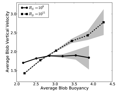
Figure 5: Average vertical velocity vs. average buoyancy in connected regions with $|B^{\prime}|\geq 2\sigma_{B^{\prime}}$ for the $R_{S}=10^{8}$ and the $R_{S}=10^{11}$ simulations. Errobars in gray are 95% bands obtained by jackknife subsampling. Data are gathered for one hundred convective times, once statistical stationarity has been reached.

It is evident that at the lowest Rayleigh number the vertical velocity of these connected regions is fairly independent of the region’s average buoyancy, thus breaking the proportionality $w\propto B^{\prime}$ for extreme values of $B^{\prime}$. At high Rayleigh number connected regions with a very high buoyancy move substantially faster than those having a lower average buoyancy. In this case the proportionality $w\propto B^{\prime}$, on average, holds fairly well.

3.3 Scalar dissipation rates

The conditional averages of temperature and salinity dissipation for the numerical experiments are reported in Figs. 6(a,b). To interpret them it is again useful to take temperature and salinity, to a good approximation, as passive scalars. The Kolmogorov-Obukhov-Corrsin scenario (e.g. ShraimanSiggia00 [12]) assumes that the dissipation of variance of a passive scalar is, on average, independent of the concentration of the scalar itself, which would yield a constant $E(\mathcal{\chi}|X)$ as a function of $X$. Sinai and Yakhot Sinai&Yakhot89 [11] suggested that concentration and dissipation of a passive scalar may be correlated. They modeled the dissipation as a parabolic function of concentration and linked this behaviour with the appearence of non-Gaussian tails. In our simulations the even parabolic expression

$$E(\chi|X)=1-\gamma+\gamma X^{2}$$ (8)

fits well the temperature and salinity dissipation data (also in this case the normalization of $X$ and of $\chi$ reduces the number of free constants in Eq. (8)). Conditional dissipation is fairly constant at $R_{S}=10^{9}$ and smoothly assumes an upward parabolic shape as the Rayleigh number increases. At low $R_{S}=10^{8}$ we find a slightly downward shape: high fluctuations of temperature or salinity are slightly less subject to dissipation than small ones. This may reflect the particular distribution of temperature and salinity inside blobs: extreme fluctuations are found mainly in the regions of low gradients at the core of the blobs, where they are protected from dissipation.

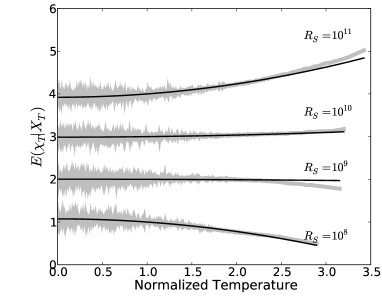
a) b)
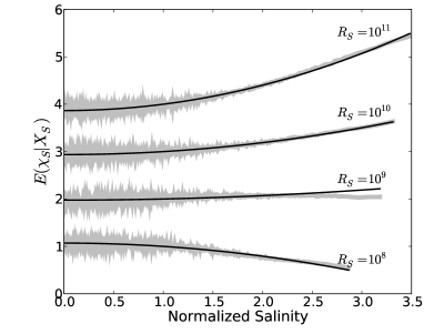
c)

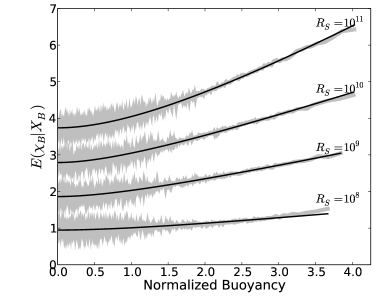
Figure 6: $(a)$ Conditional averaged dissipations of temperature and salinity, $E(\chi_{T}|X_{T})$ and $E(\chi_{S}|X_{S})$, for the four simulations at $R_{S}=10^{8},10^{9},10^{10},10^{11}$; data are gathered for one hundred convective times, once statistical stationarity has been reached. For clarity the latter three curves are shifted upward by one, two and three units, respectively. Overimposed on the numerical data is the parabolical fit (8), where the constant $\gamma$ is determined by a nonlinear least-squares fit. Only the positive normalized fluctuation half-plane is shown. For the negative half-plane even symmetry holds. $(c)$ The analogous plot for buoyancy dissipation rates, with overimposed fit (9).

Fig. 6(c) shows instead that at all Rayleigh numbers the dissipation of buoyancy is never independent of buoyancy itself. To some extent also the dissipation of buoyancy can still be interpreted as the contribution of a passive scalar. Any buoyancy fluctuation which is not aggregated into a blob is likely to be dynamically irrelevant: small buoyancy structures significantly different from rising or sinking blobs will be strongly damped by viscosity, and quickly dissipated. Therefore buoyancy in the background between the blobs is passively transported, and a parabolic shape of $E(\mathcal{\chi}_{B}|X_{B})$ at moderate values of $X_{B}$ is to be expected. For large values of $X_{B}$ the dissipation is dominated by the contribution of the blobs. The detailed distribution of buoyancy fluctuations within each blob and the distribution of blob sizes and intensities will determine the form of the tails of $E(\chi_{B}|X_{B})$ PH10 [19]. At this stage we limit ourselves to report that the numerical simulations at high Rayleigh numbers show remarcably linear tails, and postpone to a future work an in-depth investigation of the morphology of the blobs.

A simple fitting expression that allows us to join the picture inside and outside the blobs is

$$E(\chi_{B}|X_{B})=k+\frac{aX_{B}^{2}}{1+b|X_{B}|}.$$ (9)

The parameter $k$ weights the Kolmogorean part of the dissipation; $a$ is the coefficient of the quadratic component in the expression of $E(\chi_{B}|X_{B})$; $a/b$ is the asymptotic slope of the linear tails. Although the constants $k$, $a$, $b$ are functionally linked by a normalization constraint, writing this relationship explicitly is not as straightforward as in the case of the conditional expectation of the fluxes. Here we prefer to independently fit all three constants that appear in Eq. (9) with a nonlinear least-square regression to the numerical data. The results are shown in Fig. 6(c) and show very good agreement.

3.4 Agreement with the scalar distributions

Since Eq. (7) and its equivalents for temperature and salinity represent exact expressions for the scalar fluctuation amplitude distributions, computing conditional averages of the scalar fluxes and dissipations from our experimental data and substituting them into these equations, leads trivially to an almost exact overlap with the curves in Fig. 3 (not shown). When a simple dependency $E(\mathcal{F}|X)/X=X$ is used for the fluxes, together with the fits (8) (for the dissipations of temperature and salinity) and (9) (for the dissipation of buoyancy), we obtain a very good agreement with the distributions computed from the numerical simulation data, as shown by the black lines in Figs. 3(a-c). The only exceptions are the tails of the buoyancy distribution at low Rayleigh number, where the agreement is worse due to the deviations from linearity of $E(\mathcal{F}_{B}|X_{B})/X_{B}$ discussed in Sec. 3.2. Note that, when $E(\mathcal{F}|X)/X=X$ is assumed, the non-Gaussianity of the tails of the amplitude distributions is controlled by the form of the expected dissipation: the linear tails of Eq. (9) determine the exponential tails of the distributions of buoyancy fluctuations, while a dissipation independent of scalar fluctuations (as shown by temperature and salinity at low $R_{S}$), leads to Gaussian distributions.

4 Conclusions

In the numerical experiments of fingering convection reported in this letter we find sharp evidence for exponential non-Gaussian tails in the buoyancy fluctuation distributions at high Rayleigh number. In contrast, the statistics of temperature and salinity remain closer to Gaussianity even when those of buoyancy are already significantly non-Gaussian. As shown by using a custom version of a theory by Yakhot (1989), this observation can be understood in terms of the different properties of dissipation of a scalar directly creating vertical accelerations, such as buoyancy, compared to the dissipations of the individual buoyancy-changing scalars, such as temperature and salinity.

There are some analogies with the phenomenology of Rayleigh-Bénard convection, where, in the high Rayleigh number “hard-turbulence” regime, temperature fluctuations present exponential-like tails. In that setting temperature fluctuations are equivalent to buoyancy, while in fingering convection this role is played by a linear combination of temperature and salinity. We suspect that the faster appearance, in fingering convection, of non-Gaussian statistics of buoyancy, compared with those of other active scalars, may apply also to other flows with multiple active scalars.

The simple conceptual models introduced in Secs. (3.2) and (3.3) highlight the role of coherent dynamical structures in determining the vertical fluxes and dissipation of buoyancy fluctuations and consequently the appearance of non-Gaussian tails in their amplitude distribution. The same statistics for temperature and salinity are closer to what could be expected of passive scalars. The blobs of fingering convection are generated by a very different mechanism compared to the plumes of Rayleigh-Bénard convection and live in a small range of spatial scales where the effects of molecular diffusion and viscosity are very strong, but nonlinear terms are just as important. We have used a simple threshold in buoyancy to partition the flow and identify the blobs but a better identification method will be needed to characterize in detail their structure and to explore their Lagrangian properties, such as their mean free path, their characteristic life time and the dynamics of their mutual interactions.

The changes in the shape of the distributions that we observe occur gradually over a range of Rayleigh numbers spanning three orders of magnitude. The convective fluxes and other indicators (Table 1) follow cleanly simple scaling laws, with no evident breaks. This suggests that any change in the flow patterns affecting the distributions is not as dynamically important as, for example, the changes in the plumes in the analogous transition in Rayleigh-Bénard convection. Nevertheless, we are quite confident that we are not yet observing any sort of ultimate scaling regime of fingering convection. In fact, as we have argued in Sec. 3.2, the vertical convective fluxes can be modeled in terms of the equilibrium between a blob’s buoyancy and a Stokes drag. However the scalings of Table 1 imply that the Reynolds number of an individual blob increases with the Rayleigh number, and, eventually, it will significantly exceed one. At that point the dynamics will necessarily change, as the blobs will be subject to a drag having a nonlinear dependence on velocity. Whether this will simply mark a change in the slope of the scaling laws and in the form of the amplitude distributions, or if it will trigger more dramatic changes, such as the formation of the elusive staircases, remains to be seen.

References

- [1] J. S. Turner, Ann. Rev. Fluid Mech. 6, 37 (1974).
- [2] R. W. Schmitt, Ann. Rev. Fluid Mech. 26, 255 (1994).
- [3] R. W. Schmitt, Progr. Oceanogr. 56, 419 (2003).
- [4] R. W. Schmitt, J. R. Ledwell, E. T. Montgomery, K. L. Polzin, J. M. Toole, Science 308 685 (2005).
- [5] P. G. Baines and A. E. Gill, J. Fluid Mech. 37, 289 (1969).
- [6] ch. 11 in: M. E. Stern, “Ocean Circulation Physics”, Academic Press, N.Y. (1975).
- [7] W. J. Merryfield, J. Phys. Oceanogr. 30 1046 (2000).
- [8] T. Radko, J. Fluid Mech. 609 59 (2008).
- [9] R. Krishnamurti, J. Fluid Mech. 483 287 (2003).
- [10] P. Flament, Progr. Oceanogr. 54 493 (2002).
- [11] Ya. G. Sinai and V. Yakhot, Phys. Rev. Lett. 63 1962 (1989).
- [12] B. I. Shraiman and E.D. Siggia, Nature 405 639 (2000).
- [13] V. Yakhot, Phys. Rev. Lett. 63 1965 (1989).
- [14] G. Passoni, G. Alfonsi, M. Galbiati, Int. J. Numer. Methods Fluids 38 1069 (2002).
- [15] A. Parodi, J. von Hardenberg, G. Passoni, A. Provenzale, E.A. Spiegel, Phys. Rev. Lett. 92 194503 (2004).
- [16] J. von Hardenberg, A. Parodi, G. Passoni, A. Provenzale, E.A. Spiegel, Phys. Lett. A 372 2223 (2008).
- [17] E. Calzavarini et al., Phys. Rev. E 73 035301 (2006).
- [18] B. Castaing et al., J Fluid Mech. 204 1 (1989).
- [19] F. Paparella and J. von Hardenberg, in: A. M. Greco, S. Rionero, T. Ruggeri (Eds.) Proceedings of WASCOM 2009, World Scientific, in press (2010).