IRFU-10-17

Z boson transverse momentum spectrum from the lepton angular distributions

M. Boonekamp (CEA), M. Schott (CERN)

  Abstract — In view of recent discussions concerning the possibly limiting energy resolution systematics on the measurement of the Z boson transverse momentum distribution at hadron colliders, we propose a novel measurement method based on the angular distributions of the decay leptons. We also introduce a phenomenological parametrization of the transverse momentum distribution that adapts well to all currently available predictions, a useful tool to quantify their differences.

 

1 Introduction

The transverse momentum distribution of heavy particles at hadron colliders is a longstanding subject, first discussed in the context of QCD. Formalisms were developed to predict this distribution, based on analytical or numerical methods (soft gluon resummation theory [1, 2, 3, 4], or parton shower Monte Carlo programs [5, 6] respectively). In both cases, the shape of the distribution is predicted qualitatively, but the full result depends on a limited number of free parameters which need to be extracted from measurement.

The distribution is of physical interest for many reasons. Firstly, the measurement of the overall vector boson production cross sections is considered an important test of perturbative QCD, theoretical predictions now being available up to NNLO [7]. In the context of the total cross section measurement, the kinematic cuts imposed on the decay leptons, reflecting the detector geometric acceptance, require that the observed event rate be corrected by a factor compensating this loss of acceptance. The fraction of lost events must be precisely controled so that the final result contains no significant bias. This in turn implies that the lepton kinematic distributions, and hence the vector boson ones from which they derive, need to be known both inside and outside the selected region.

Another application is the precise measurement of the W boson mass [8]. The decay lepton transverse momentum distribution, or the W boson transverse mass distribution from which this fundamental parameter is extracted, is a complicated quantity resulting in part from the W boson transverse momentum spectrum, $d\sigma_{W}/dp_{T}$. The increasing precision of the measurements of $M_{W}$ puts ever stronger constraints on the knowledge of $d\sigma_{W}/dp_{T}$. An important tool for constraining this distribution is the study of the Z boson transverse momentum spectrum, $d\sigma_{Z}/dp_{T}$.

The recent measurements performed at the Tevatron are increasingly sensitive to the detector energy resolution, which needs to be precisely “subtracted”, or unfolded from the observed distribution to derive an estimate of the true one. This issue will become much more important at the LHC, given the high expected statistics. An alternative variable, $a_{T}$, was introduced recently [9] as a replacement for $p_{T}$. Its advantage is that it is negligibly sensitive to the energy resolution, while still a good probe of resummation or parton shower mechanisms.

In this paper, we propose a novel method that shares the insensitivity of $a_{T}$ to the energy resolution, while remaining a true $p_{T}$ measurement. The method is based on the measured angular distributions of the $Z$ boson decay leptons, which, together with the well known Z boson mass, are sufficient to extract the $p_{T}$ distribution.

In the following, we first introduce a convenient parametrization of the $p_{T}$ distribution. It depends on three intuitive parameters, and adapts well to the available predictions. It represents a practical tool to quantify differences between predictions, as well as for the measurement itself. We then outline the measurement method, and give examples of its performance in a simplified form. We conclude with some caveats and perspectives concerning the use of this method in future measurements.

2 A parametrized form for the $p_{T}$ distribution

The parametrization we propose relies on a number of simple arguments. Consider Z boson production at high energy, and at given mass and rapidity, so that the parton momentum fractions at the hard vertex are small and fixed. In the low transverse momentum region, the repeated gluon emission in the initial state generates a gaussian transverse momentum distribution. Along both the $x$ and $y$ axes, this ”random walk” leads to a distribution proportional to

$$f(p_{x,y};\sigma_{PS})\,\,dp_{x,y}\sim e^{-\frac{p^{2}_{x,y}}{2\sigma_{PS}^{2}}}\,\,dp_{x,y}.$$

The $\sigma_{PS}$ parameter represents the spread of the $p_{X,Y}$ distribution after all emissions and, in a naive picture, could be seen as representing the average number of emitted gluons times their average transverse momentum: $\sigma_{PS}\sim\sqrt{N_{g}}\times p^{g}_{x,y}$. Moving to polar coordinates, the distribution becomes:

$$f(p_{x};\sigma_{PS})\,\,f(p_{y};\sigma_{PS})\,\,dp_{x}\,\,dp_{y} \sim e^{-\frac{p^{2}_{x}}{2\sigma_{PS}^{2}}}\,\,e^{-\frac{p^{2}_{y}}{2\sigma_{PS}^{2}}}\,\,dp_{x}\,\,dp_{y}$$

$$= e^{-\frac{p_{T}^{2}}{2\sigma_{PS}^{2}}}\,\,p_{T}\,\,dp_{T}\,\,d\phi\,\,\equiv\,\,g_{1}(p_{T};\sigma_{PS})\,\,dp_{T}.$$

after a trivial azimuthal integral. At higher $p_{T}$, the shape is dominated by a power law behaviour representing the parton density functions (PDFs) and the perturbative matrix element:

$$g_{2}(p_{T};a)\sim 1/p_{T}^{\alpha}.$$

The transition between the two descriptions is controled by a parameter $n$, defined such that $p_{T}^{match}=n\times\sigma_{PS}$. As for the definition of the Crystal Ball function [10], it satisfies smoothness conditions (the function and its derivative are continuous). The complete parametrization is, forgetting an overall normalization factor:

$$g(p_{T};\sigma_{PS},\alpha,n) = p_{T}\,\,e^{-\frac{p_{T}^{2}}{2\sigma_{PS}^{2}}},\,\,\,\,\,\,p_{T}<n\times\sigma_{PS};$$ (1)

$$= p_{T}\,\,\frac{(\frac{\alpha}{n})^{\alpha}\,e^{-n^{2}/2}}{(\frac{\alpha}{n}-n+\frac{p_{T}}{\sigma_{PS}})^{\alpha}},\,\,\,p_{T}>n\times\sigma_{PS};$$

where the parameters $\alpha$, $n$, and $\sigma_{PS}$ are all positive definite. Fitted to various generator level $\frac{1}{\sigma}\frac{d\sigma}{dp_{T}}$ distributions, this parametrisation shows a nice behaviour in the range in $0<p_{T}<50$ GeV. Over a wider range, the agreement slightly deteriorates, due to the fact that the high $p_{T}$ power law with a constant power is a crude approximation. Both PDFs and matrix element’s power depend on the scale $Q$ of the process, which is related to $p_{T}$. The fit quality could be improved by introducing a running power law, $\alpha(Q^{2})$, at the cost of additional free parameters.

Figure 1 shows the parametrisation fitted to distributions obtained using the Monte Carlo event generators PYTHIA [5], MC@NLO [11], and two versions of RESBOS [2, 3, 12]: the default computation, and a computation including small-$x$ broadening effects. All distributions are obtained at $\sqrt{s}=14$ TeV, $Q=M_{Z}$ and $y_{Z}=0$. The fit quality is good, with $\chi^{2}\sim 1$ in all cases.

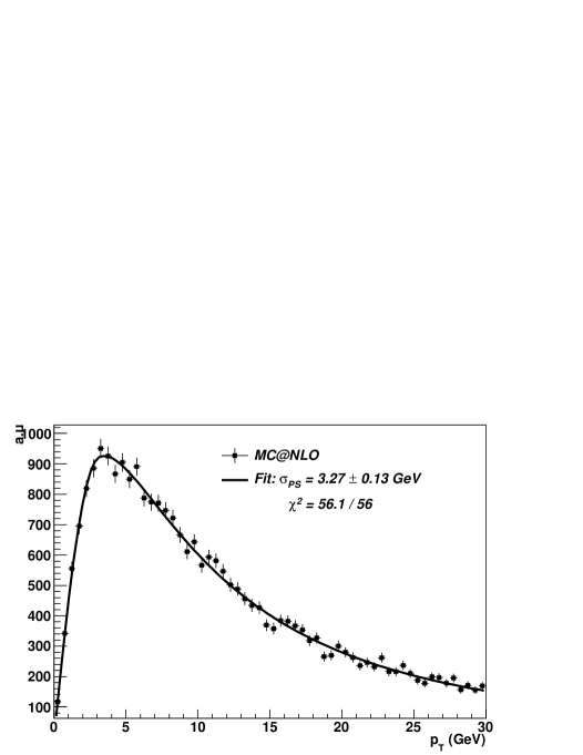
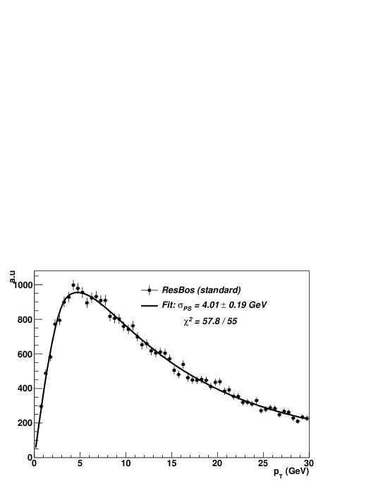
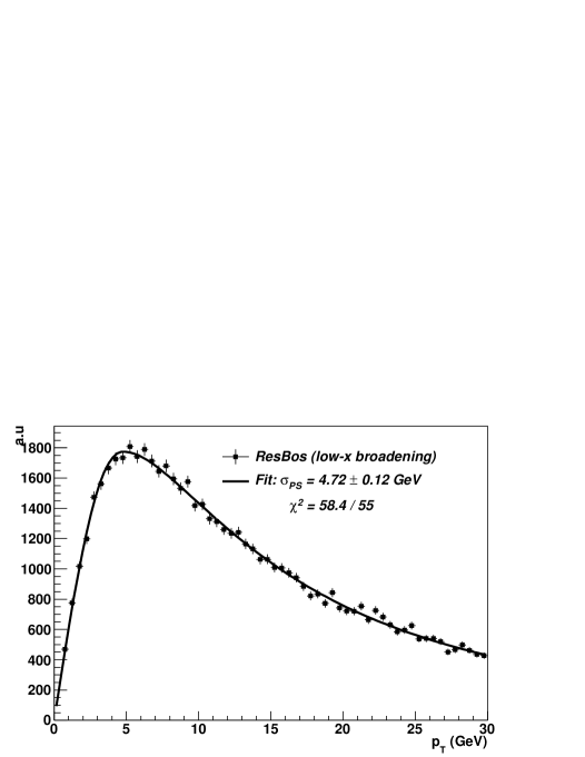
Figure 1: Generator level $p_{T}$ distribution, at $\sqrt{s}=14$ TeV, $Q=M_{Z}$ and $y_{Z}=0$ , as predicted by PYTHIA 1, MC@NLO 1, the standard RESBOS 1, and by the version including low-$x$ broadening effects 1.

It is interesting to study the dependence of the $\sigma_{PS}$ parameter as a function of rapidity, as illustrated in Figure 2. The standard RESBOS prediction shows falling values of this parameter at higher rapidity, an effect generally expected from the decreasing phase space on one side of the parton shower. The modified version, however, shows an increase of this parameter, resulting from the low-$x$ effects. It would be interesting to measure this dependence in the current and forthcoming hadron collider data.

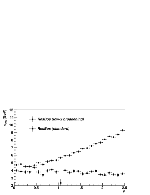
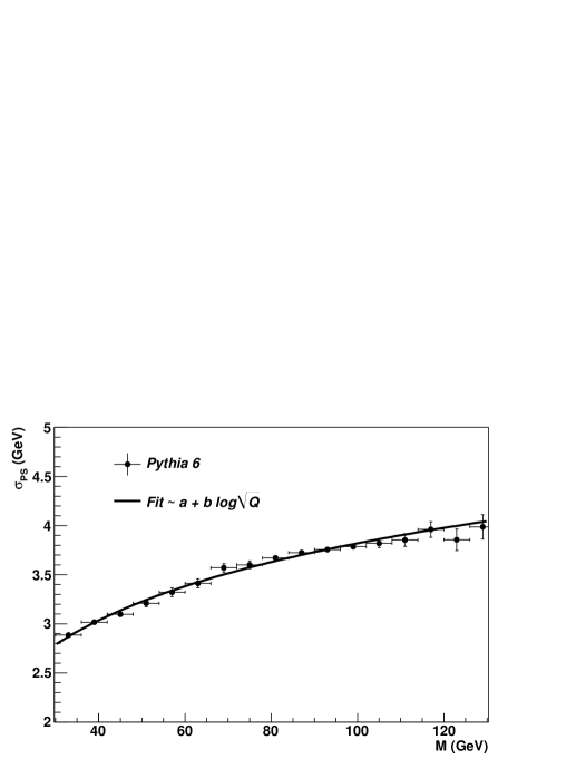
Figure 2: Rapidity dependence of $\sigma_{PS}$, as predicted by the standard RESBOS, and by the version including low-$x$ broadening effects 2; mass dependence of $\sigma_{PS}$, as predicted by PYTHIA 2.

Finally, one can study the $Q$ dependence of the $\sigma_{PS}$ parameter. As stated above, it is naively proportional to $\sqrt{N_{g}}$, the number of gluons emitted in the initial state. $N_{g}$ is, on the other hand and according to the Altarelli-Parisi evolution equations [13, 14, 15], proportional to the logarithm of the scale variation between the original proton and the hard process, $N_{g}\sim\log(Q^{2})$. Plotting $\sigma_{PS}$ as a function of $Q$, taken to be the boson invariant mass event by event, shows a behaviour following $\sigma_{PS}\sim\sqrt{\log(Q^{2})}$ as expected in this simple picture.

3 $p_{T}$ spectrum from the angular distributions

3.1 Methodology

The proposed measurement procedure is suggested by observing that at given transverse momentum and at fixed mass, the $Z$ boson angular distribution can be written as the product of the lepton angular distribution in the $Z$ rest frame, and a factor relating the lepton angles in the rest frame and laboraty frame. For simplicity, we consider the azimuthal angular distribution only:

$$\left({\frac{d\sigma}{\Delta\phi}}\right)_{p_{T}}=\left(\frac{d\sigma}{d\phi^{*}}\right)_{p_{T}}\times\left(\frac{d\phi^{*}}{d\Delta\phi}\right)_{p_{T}}$$ (2)

Above, $\phi^{*}$ is the azimuthal angle in the rest frame, and $\Delta\phi=\phi_{1}-\phi_{2}$ the angular separation in the laboratory frame. The transverse momentum distribution can be inferred by noting that the overall $\Delta\phi$ distribution is the integral of the above over the $p_{T}$ distribution:

$$\frac{d\sigma}{d\Delta\phi}=\int\left(\frac{d\sigma}{\Delta\phi}\right)_{p_{T}}\frac{d\sigma}{dp_{T}}dp_{T}$$ (3)

In Eq. 2, the first factor on the right hand side has a well defined form, and can be computed perturbatively. In the Collins-Soper frame [16], one finds:

$$\left(\frac{d\sigma}{d\Omega}\right)_{p_{T}}\sim 1+\cos^{2}\theta^{*}+(\frac{1}{2}-\frac{3}{2}\cos^{2}\theta^{*})\,\,A_{0}+\cos\theta^{*}\sin\theta^{*}\cos\phi^{*}\,\,A_{1}+\frac{1}{2}\sin^{2}\theta^{*}\cos 2\phi^{*}\,\,A_{2}$$ (4)

where the coefficients $A_{i}$ can be calculated perturbatively and are functions of the kinematic variables $s$, $y$, $p_{T}$. The second factor is purely kinematic. In the simplest case where the system is purely transverse (all rapidities are 0 and momenta are purely transverse), the relation between $\phi^{*}$ and $\Delta\phi$ takes the following form:

$$\phi^{*}=\cos^{-1}\left(\frac{1}{\beta}\sqrt{\frac{2\beta^{2}-\cos\Delta\phi}{1-\cos\Delta\phi}}\right)$$ (5)

where $\beta=\frac{p_{T}}{E}$, and from which the the derivative $\frac{d\phi^{*}}{d\Delta\phi}$ in Equation 2 can be computed. According to the above, the $\Delta\phi$ distribution is directly sensitive to $p_{T}$: small values of $\Delta\phi$ indicate large $p_{T}$ values. In the general case, the polar decay angles complicate the picture significantly, as at finite but modest $p_{T}$, small $\Delta\phi$ values are also obtained from forward decays ($|\eta|\gg 0$), leading to a small projection of the lepton pair opening angle in the transverse plane. In addition, the expressions have to be integrated over the $Z$ boson lineshape, so that in practice we have to extract the factors from large Monte Carlo generated event samples. For the sake of simplicity, we stick to Eq. 3 and compute the the $\Delta\phi$ distribution at given $p_{T}$ integrating over all other relevant variables:

$$\left(\frac{d\sigma}{\Delta\phi}\right)_{p_{T}}=\int\left(\frac{d\sigma}{\Delta\phi}\right)_{p_{T};m,y,\eta}dm\,dy\,d\eta$$ (6)

For the analysis, we use a sample of $10^{6}$ events, generated with MC@NLO. While this approximation is not optimal as the lepton rapidities are also measured, providing additional information which is not exploited here, it is sufficient for the purpose of demonstration. Statistical sensitivities discussed here should thus be understood as conservative.

The integrated azimuthal angular $\Delta\phi$ distribution prediction for MC@NLO is shown in Figure 4, requiring that both decay leptons have a transverse momentum above $20$ GeV and a pseudo-rapidity $\eta$ smaller than $2.5$, as generic acceptance cuts applied by the LHC experiments ATLAS and CMS. The corresponding $\Delta\phi$ distribution vs. the transverse momentum distribution of the Z is shown in Figure 4. It can be interpreted as a matrix $M$, relating a given $p_{T}$ distribution to a $\Delta\phi$ distribution, via

$$\Delta\phi_{i}=M_{ij}\cdot{p_{T}}_{j}$$ (7)

where $i$ and $j$ are the numbers of bin of the $\Delta\phi$ and $p_{T}$ distribution. It is required that each row of $M$ is normalized to unity. The basic idea is to use the measured $\Delta\phi$ distribution to estimate the $p_{T}$ distribution, exploiting their relation through the matrix $M$. The inverse matrix $M^{-1}$ directly relates $p_{T}$ distribution to the measured $\vec{\Delta\phi}$ by a simple matrix multiplication. The matrix $M$ has significant off-diagonal entries and a non-uniform distribution of values on the diagonal. Hence, the inversion of $M$ and the statistical fluctuations in $\vec{\Delta\phi}$ induce large fluctuations in $\vec{p_{T}}$ and therefore sub-optimal results.

Therefore it was chosen to adjust the MC predicted $p_{T}$ distribution iteratively to minimize the difference in the corresponding ${\Delta\phi}_{MC}$ distribution, which is calculated via Equation 7, and the measured ${\Delta\phi}_{Data}$. The difference is expressed as a $\chi^{2}$-value, i.e.

$$\chi^{2} := \sum_{i}\frac{{\Delta\phi}_{Data,i}-{\Delta\phi}_{MC,i}}{\sigma^{2}_{MC,i}}$$ (8)

$$= \sum_{i}\frac{{\Delta\phi}_{Data,i}-M_{ij}\cdot{p_{T,j}}}{\sigma^{2}_{MC,i}}$$ (9)

It was assumed that the statistical uncertainty $\sigma$ is purely due to the measurement, as the Monte Carlo based observables can be theoretically defined with infinite statistics. The parameters to be varied in Equation 8 are all entries of the $p_{T}$ distribution, i.e. in realistic scenarios more than 30. This relatively large number of free fitting parameters dramatically hinders the minimization of Equation 8, especially when the statistics of the measured $\Delta\phi$ distribution is limited. Hence it was chosen to use $f(p_{T},\sigma_{PS},\alpha,n)$, defined in Equation 1, to model the $p_{T}$ distribution, i.e. using only three free parameters $\sigma_{PS},\alpha$ and $n$ during the $\chi^{2}$ -minimization procedure. It has been shown in Section 2 that the parameterization of the $p_{T}$ spectrum via Equation 1 provides an adequate description up to statistics of at least $5.10^{4}$ events, which we assume in the present analysis.

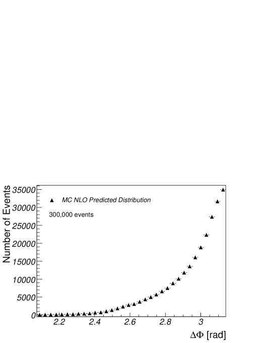
Figure 3: Opening-angle distribution for two Z boson decay leptons.

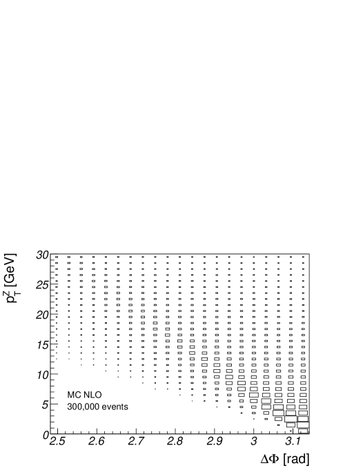
Figure 4: Distribution of the opening-angle between the two leptons and the $p_{T}$ distribution of the Z boson.

3.2 Expected Precision

As already mentioned in Section 1, a prominent systematic uncertainty in the standard measurement of the $p_{T}$ is induced by the uncertainty on the decay lepton momentum measurement. In contrast, the presented approach has only a very weak dependence on the momentum measurement, but relies on the measurement of $\Delta\Phi$, which has in general extremely high precision in most collider experiments. The expected precision of modern detectors, like ATLAS or CMS, is a magnitude smaller than the required binning in the $\Delta\Phi$ distribution. For this reason, the $\Delta\Phi$ distribution is not required to be unfolded, which is an additional advantage compared to the standard measurement.

The uncertainties on the lepton transverse momentum measurement can be parameterized to first order as

$$p_{T}\rightarrow a\cdot p_{T}+\mathrm{Gauss}(m,\sigma)$$

where $a$ is a scale parameter, $m$ is an offset parameter of and $\sigma$ is the width of an additional Gaussian (resolution) uncertainty. The scale parameter $a$ is assumed to have an uncertainty of $1\%$, the resolution parameter $\sigma$ is assumed to have an uncertainty of 300 MeV. Moreover, we assume a systematic shift of $2\times 10^{-3}rad$ on the $\Delta\Phi$ measurement. The latter assumption is rather conservative, keeping in mind the precise $\Delta\Phi$ resolution.

With this assumptions of systematic uncertainties, we can compare both measurement techniques. Table 1 shows the comparison of function parameters $\alpha,\sigma,n$ of Equation 1 and its maximum $max$ for different measurement methods and systematic uncertainties. Standard denotes that the parameter values have been obtained by directly fitting the predicted transverse momentum distribution. $\Delta\Phi$ denotes that the corresponding values have been obtained with fitting the opening angle distribution. Ideal labels that a perfect detector has been assumed, i.e. with perfectly known resolution, while distorted assumes the stated uncertainties on the detector resolution. The given values are based on 500.000 selected Z boson events in a specified leptonic decay channel, generated with MC@NLO.

The parameters in the ideal, standard column are the reference values for the comparisons. The values of the $\Delta\Phi$ approach agree within their statistical uncertainties to the reference values. Moreover, the assumed systematic uncertainty on the $\Delta\Phi$ measurement has no significant effect of the fit results. This is not the case for the distorted standard measurement, where a significant difference compared to the ideal measurement can be observed. The statistical precision of the $\Delta\Phi$-approach is reduced less, by a factor of $2$. Such a decrease is expected due to the integration over rapidity and the mass of the Z boson and hence not all statistical information used. This can be partially recovered when taken the rapidity information into account during the fitting procedure, or when restricting the analysis to a smaller rapidity range, e.g. $|y|<1.0$. Nevertheless, the systematic difference between the standard measurement is worse compared to the statistical uncertainty of the $\Delta\Phi$-approach.

Parameter	standard	standard measurement	$\Delta\Phi$ approach	$\Delta\Phi$ approach
	(ideal)	(distorted)	(ideal)	(distorted)
$max$	3.89 (0.02)	4.04 (0.02)	3.90 (0.04)	3.90 (0.04)
$\sigma$	3.25 (0.03)	3.10 (0.05)	3.22 (0.8)	3.23 (0.09)
$\alpha$	0.90 (0.01)	0.85 (0.01)	0.89 (0.02)	0.91 (0.03)
$n$	3.57 (0.02)	3.94 (0.04)	3.58 (0.06)	3.59 (0.06)

Table 1: Comparison of function parameters $\alpha,\sigma,n$ and the maximum of the function for different measurement methods and systematic uncertainties. The statistical uncertainties are given in parenthesis.

3.3 Comparison of different Monte Carlo Generators

As previously discussed, the values of the matrix $M$ are predicted by a Monte Carlo generator. In this section, it will be discussed to which extent the final $p_{T}$ measurement is independent of a specific Monte Carlo generator program. In order to test this independence, an attempt was made to predict the $p_{T}$ spectrum of one generator using the predicted matrix $M$ of a second generator. Again, it was chosen that the matrix is based on MC@NLO. The $p_{T}$ and $\Delta\Phi$ spectra used for the comparison and fitting, respectively, are taken from HERWIG, RESBOS, and RESBOS including the x-broadening effect. Each spectra is based on 50.000 reconstucted Z boson events, corresponding roughly to an integrated luminosity of ${\cal L}=\int 100\,\mbox{pb}^{-1}$ at the LHC at a collision energy of $7$ TeV. The resulting $p_{T}$ spectra, including the functional description obtained with a direct fit and via the $\Delta\Phi$ measurement are shown for the different generators in Figure 5. The corresponding fitting parameters are shown in Table 2.

Parameter	MC@NLO	HERWIG	RESBOS	RESBOS
				(small x)
$\sigma_{Truth}$	3.31 (0.09)	3.80 (0.17)	4.27 (0.11)	5.50 (0.13)
$\sigma_{\Delta\Phi}$	3.14 (0.30)	3.70 (0.44)	4.45 (0.29)	5.70 (0.28)
$\alpha_{Truth}$	0.90 (0.03)	0.92 (0.04)	0.97 (0.03)	1.07 (0.03)
$\alpha_{\Delta\Phi}$	0.83 (0.09)	0.88 (0.11)	0.99 (0.07)	1.07 (0.07)
$n_{Truth}$	3.55 (0.09)	3.81 (0.14)	3.62 (0.14)	4.04 (0.25)
$n_{\Delta\Phi}$	3.86 (0.20)	4.12 (0.39)	3.96 (0.40)	4.84 (0.77)
$max_{Truth}$	3.95 (0.07)	4.34 (0.10)	4.48 (0.09)	5.50 (0.13)
$max_{\Delta\Phi}$	4.11 (0.14)	4.50 (0.22)	4.70 (0.16)	5.78 (0.20)

Table 2: Comparison of function parameters $\alpha,\sigma,n$ and the maximum of the function for different Monte Carlo generator programs. The subscript truth denotes that the function has been directly fitted to the predicted transverse momentum distribution, while the subscript $\Delta\Phi$ denotes that the corresponding values have been obtained with fitting the opening angle distribution. The values correspond to 50.000 selected events.

The $\Delta\Phi$ fitted values agree within their statistical uncertainty to the values, obtained by a direct fit to the truth $p_{T}$ distribution. As already mentioned in the previous section, the statistical precision and also the systematic differences are mainly due to the integration over the Z boson rapidity.

Figure 5: Fitted function for different Monte Carlo generator programs: MC@NLO (a), HERWIG (b),RESBOS (c), RESBOS with x-broading (d). The dashed function has been directly fitted to the Monte Carlo predicted transverse momentum distribution, while the solid function line has been obtained with by the opening angle distribution. The errors and therefore the quoted likelihoods correspond to 50.000 reconstructed events..

3.4 X-Broadening Effects

As a final example we want to demonstrate that the presented $\Delta\Phi$ based $p_{T}$ spectrum measurement can be also used to test the x-broadening prediction at LHC for early data, i.e. small integrated luminosities.

Instead of directly measuring the $p_{T}$ spectrum to test the x-broadening effect, we propose to measure the maximum of the $p_{T}$ spectrum for different intervals of the Z-boson rapidity. Figure 7 shows the predicted $p_{T}$ spectra for different $y_{Z}$. Larger Z boson rapidities $y_{Z}$ test smaller x-regimes of the interacting partons. Hence it is expected that the x-broadening enhances for larger $y_{Z}$ values, i.e. the maximum the $p_{T}$ shifts to larger values. The measurement of the maximum dependence of the $p_{T}$ on $y_{Z}$ does not only allow to see a possible x-broadening effect, but also to constrain some model parameters.

To test the $\Delta\Phi$ based measurement, we again assume a statistics of $50.000$ reconstructed Z boson decays, distributed in five rapitity intervals ($[0,0.5]$, $[0.5,1.0]$, $[1.0,1.5]$, $[1.5,2.0]$ and $[2.0,2.5]$). In each interval, we perform the $\Delta\Phi$ based fit and extract the maximum of the corresponding $p_{T}$ distribution. The results are shown in Figure 7. It becomes evident that we can distinguish between the standard prediction and the small-x prediction using the $\Delta\Phi$ based fit on a relatively small data sample.

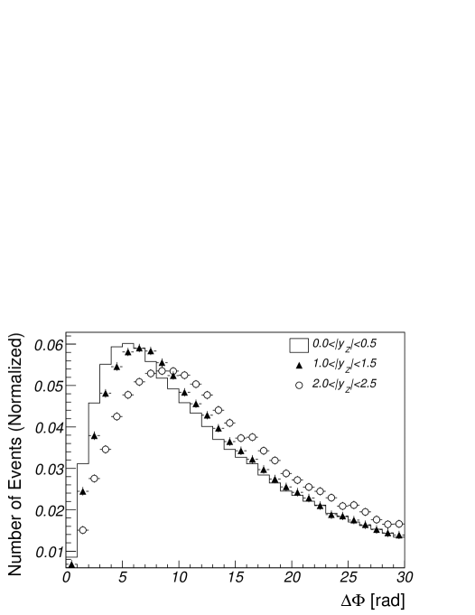
Figure 6: Transverse Momentum Spectrum for different rapidity ranges of the Z boson

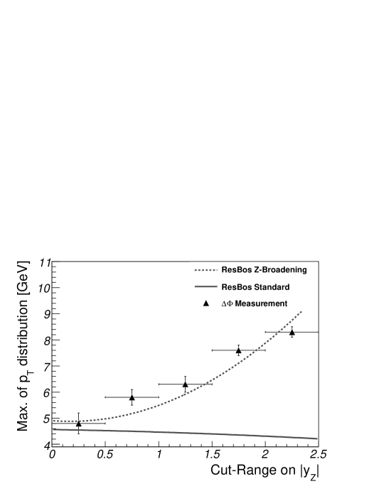
Figure 7: X-Broadening determination with 50.000 reconstructed events.

4 Perspectives

The present work has two components. First, a phenomenological, three-parameter parametrization of the heavy boson $p_{T}$ distribution was introduced, which proved sufficiently versatile to describe the available theoretical predictions. This function has many applications, in quantifying differences between predictions and assisting the measurement procedure.

Secondly, we propose a measurement method that is free of any energy resolution systematics, while remaining a measurement of the $p_{T}$ distribution. The result can thus be directly compared to theoretical predictions of this quantity. We presented here a simplified version of this algorithm, based on a map representing the $\Delta\phi$ distribution at given $p_{T}$. The map was integrated over rapidity for simplicity of this presentation, at the cost of some statistical power. A complete treatment will have to account for the lepton pseudo-rapidity event by event.

The computation of this map was performed by Monte Carlo simulations, and relies on the well known $Z$ boson mass distribution, on kinematics, and on the $\phi^{*}$ distribution in the Collins-Soper frame, which can be computed perturbatively with good precision. The uncertainty induced by this assumption can be expected to be small, but will have to be quantified by further study. A realistic measurement will need sufficient statistics, typically $O(50000)$ events, and would benefit from an analytical calculation of the map.

In summary, we have proposed here a method that takes as input reliably computed quantities on the theoretical side, and precisely measured angles on the experimental side. The resolution of the lepton energy measurment enters only through the kinematic selections, with negligible effect. The statistical power of the method is about a factor two less than a direct measurement, but we expect that the reduced systematic uncertainties involved here will compensate for this in the long term.

5 Acknowledgements

One of the authors (M.S) gratefully acknowledges CEA/IRFU for support.

References

- [1] J. C. Collins, D. E. Soper and G. Sterman, Nucl. Phys. B 250 (1985) 199.
- [2] G. A. Ladinsky and C. P. Yuan, Phys. Rev. D 50, 4239 (1994) [arXiv:hep-ph/9311341].
- [3] C. Balazs and C. P. Yuan, Phys. Rev. D 56, 5558 (1997) [arXiv:hep-ph/9704258].
- [4] F. Landry, R. Brock, P. M. Nadolsky and C. P. Yuan, Phys. Rev. D 67, 073016 (2003) [arXiv:hep-ph/0212159].
- [5] T. Sjostrand, S. Mrenna and P. Z. Skands, JHEP 0605, 026 (2006) [arXiv:hep-ph/0603175].
- [6] G. Corcella et al., arXiv:hep-ph/0210213.
- [7] K. Melnikov and F. Petriello, Phys. Rev. D 74, 114017 (2006) [arXiv:hep-ph/0609070].
- [8] N. Besson, M. Boonekamp, E. Klinkby, T. Petersen and S. Mehlhase [ATLAS Collaboration], Eur. Phys. J. C 57, 627 (2008) [arXiv:0805.2093 [hep-ex]].
- [9] M. Vesterinen and T. R. Wyatt, Nucl. Instrum. Meth. A 602, 432 (2009) [arXiv:0807.4956 [hep-ex]].
- [10] J. Gaiser, “Charmonium Spectroscopy From Radiative Decays Of The J / Psi And Psi-Prime,” (PhD thesis), SLAC-R-255.
- [11] S. Frixione and B. R. Webber, arXiv:0812.0770 [hep-ph].
- [12] S. Berge, P. M. Nadolsky, F. Olness and C. P. Yuan, Phys. Rev. D 72, 033015 (2005) [arXiv:hep-ph/0410375].
- [13] V. N. Gribov and L. N. Lipatov, Sov. J. Nucl. Phys. 15, 438 (1972) [Yad. Fiz. 15, 781 (1972)].
- [14] G. Altarelli and G. Parisi, Nucl. Phys. B 126, 298 (1977).
- [15] Y. L. Dokshitzer, Sov. Phys. JETP 46, 641 (1977) [Zh. Eksp. Teor. Fiz. 73, 1216 (1977)].
- [16] J. C. Collins and D. E. Soper, Phys. Rev. D 16, 2219 (1977).