Ultradeep $K_{S}$ Imaging in the GOODS-N

Abstract

We present an ultradeep $K_{S}$-band image that covers $0.5\times 0.5$ deg² centered on the Great Observatories Origins Deep Survey-North (GOODS-N). The image reaches a 5 $\sigma$ depth of $K_{S,\rm AB}=24.45$ in the GOODS-N region, which is as deep as the GOODS-N Spitzer Infrared Array Camera (IRAC) 3.6 $\mu$m image. We present a new method of constructing IRAC catalogs that uses the higher spatial resolution $K_{S}$ image and catalog as priors and iteratively subtracts fluxes from the IRAC images to estimate the IRAC fluxes. Our iterative method is different from the $\chi^{2}$ approach adopted by other groups. We verified our results using data taken in two different epochs of observations, as well as by comparing our colors with the colors of stars and with the colors derived from model spectral energy distributions (SEDs) of galaxies at various redshifts. We make available to the community our WIRCam $K_{S}$-band image and catalog (94951 objects in 0.25 deg²), the Interactive Data Language (IDL) pipeline used for reducing the WIRCam images, and our IRAC 3.6 to 8.0 $\mu$m catalog (16950 objects in 0.06 deg² at 3.6 $\mu$m). With this improved $K_{S}$ and IRAC catalog and a large spectroscopic sample from our previous work, we study the color-magnitude and color-color diagrams of galaxies. We compare the effectiveness of using $K_{S}$ and IRAC colors to select active galactic nuclei (AGNs) and galaxies at various redshifts. We also study a color selection of $z=0.65$–1.2 galaxies using the $K_{S}$, 3.6 $\mu$m, and 4.5 $\mu$m bands.

1. Introduction

Deep near-infrared (NIR) imaging is essential for understanding galaxy evolution at high redshifts. One of its key applications is the determination of galactic mass. NIR luminosity is the best tracer of galactic stellar mass because it is less affected by extinction and young stars. This role is traditionally played by deep ground-based $K$-band imaging (e.g., Cowie et al., 1994; Kauffmann & Charlot, 1998; Brinchmann & Ellis, 2000). An important reason for this is that the $K$-correction at $K$-band is small across a broad range of redshifts and is relatively invariant against galaxy types compared to the other two NIR bands ($J$ and $H$, see, e.g., Keenan et al., 2010). Recently, the high sensitivity of the Spitzer Infrared Array Camera (IRAC, Fazio et al., 2004) adds additional powerful wavebands for this purpose (e.g., Fontana et al., 2006; Pérez-González et al., 2008; Elsner et al., 2008). However, ground-based $K$-band imaging remains important because of the ease of observations.

In order to study galaxy formation and evolution, we have been carrying out deep NIR imaging in the Great Observatories Origins Deep Survey-North (GOODS-N, Giavalisco et al., 2004). In Barger, Cowie, & Wang (2008, hereafter B08) we presented a deep $K_{S}$-band catalog in the GOODS-N obtained with the Wide-field InfraRed Camera (WIRCam) on the 3.6 m Canada-France-Hawaii Telescope (CFHT). The WIRCam image was used by Wang et al. (2007) to study an optically faint submillimeter galaxy. The catalog was used by Cowie & Barger (2008) to construct a mass-selected sample of galaxies at $z<1.5$ with an AB magnitude limit of 23.4. We have since added more data to the WIRCam $K_{S}$ imaging and slightly improved the reduction. In this paper we present the new image and a new $K_{S}$ catalog. In order to achieve a more complete sampling of galaxy mass at high redshifts, we have also constructed a new 3.6 to 8.0 $\mu$m catalog based on Spitzer IRAC images in the GOODS-N (M. Dickinson et al., in preparation), which we also present here.

Colors in the Spitzer IRAC bands are used to study the redshifts of galaxies, especially optically faint ones (e.g., Pope et al., 2006; Wang et al., 2007; Devlin et al., 2009; Marsden et al., 2009). This is largely based on the rest-frame 1.6 $\mu$m bump in galactic spectral energy distributions (SEDs), which is caused by the H^- opacity minimum in the stellar photosphere (Simpson & Eisenhardt, 1999; Sawicki, 2002). IRAC colors are also used for separating active galactic nuclei (AGNs) from galaxies (Lacy et al., 2004; Stern et al., 2005, see also Hatziminaoglou et al., 2005; Sajina, Lacy, & Scott, 2005). In B08 we studied the effectiveness of using IRAC colors to select AGNs and galaxies at various redshifts based on a large spectroscopic sample, and we pointed out the limitations in these selections. With our improved color measurements in the IRAC and $K_{S}$ bands, we revisit and discuss these issues.

We describe the observations in § 2, the data reduction in § 3, the reduction quality in § 4, and a $K_{S}$ selected catalog in § 5. We present in § 6 a new method of constructing IRAC catalogs based on the $K_{S}$-band image and catalog, and we evaluate the performance of our new method. In § 7 we describe the general properties of the $K_{S}$ and IRAC catalog, including its overlap with other multiwavelength catalogs, the $K_{S}$ and IRAC color-magnitude diagrams and color-color diagrams. We summarize our results in § 8. The images and catalog data from this work will be available online. All fluxes in this paper are $f_{\nu}$. All magnitudes are in AB system, unless otherwise stated, where an AB magnitude is defined as $\rm AB=23.9-2.5\log(\mathrm{Jy})$.

2. WIRCam Imaging Observations

Ultradeep $K_{S}$-band imaging observations of the Hubble Deep Field-North (HDF-N), including the GOODS-N and flanking fields, were carried out with WIRCam on the CFHT. WIRCam consists of four $2048\times 2048$ HAWAII2-RG detectors covering a field of view of $20\arcmin\times 20\arcmin$ with a $0\farcs 3$ pixel scale. The observations were made in semesters 2006A, 2007A, and 2008A by two groups. A Canadian group led by Luc Simard obtained 11.5 hr of integration in 2006A. Our group based in Hawaii obtained 37.9 hr of integration between 2006A and 2008A, bringing the total integration to 49.4 hr. To recover the gap between the sensors and bad pixels, all exposures were dithered with various offsets ranging from $\pm 0\farcm 5$ to $\pm 1\farcm 5$ along R.A. and Dec. The dither patterns were changed after each semester in order to minimize artifacts caused by flat fielding or by sky subtraction. After each 0.5 to 1 hr of dithered observations, the dither centers were offset by up to $\pm 6\arcmin$ to further broaden the area coverage and smooth out the distribution of integration time. The observations were carried out by the CFHT in queue mode with weather monitoring. Nearly all of the data were taken under photometric conditions. A small fraction ($<10\%$) of the data were taken under thin cirrus, so we have down-weighted them (see next section). Typical seeing for the observations is between $0\farcs 7$ and $0\farcs 8$ (FWHM). Images taken under $>1\arcsec$ seeing were not used in the reduction.

3. Data Reduction

In order to reduce imaging data taken with WIRCam and similar cameras, we have developed an Interactive Data Language (IDL) based reduction pipeline—SIMPLE Imaging and Mosaicking PipeLinE (SIMPLE). Here we describe the SIMPLE reduction of the WIRCam data.

3.1. Removal of Instrumental Features

The WIRCam images were reduced chip by chip. Because of the rapidly varying sky color in the NIR, only dithered images taken within $\sim 0.5$ hr were grouped and reduced together. A group of raw images were first corrected for nonlinearity in the instrumental response with correction coefficients provided by the CFHT (C.-H. Yan, 2008, priv. comm.). The images were then normalized, median-combined to form a sky flat field, and flattened with that. In the flattened images, objects were detected and masked back in the raw images. The masked raw images were normalized again by taking into account the locations of the masked pixels and then median-combined to form a second sky flat. This was used as the final flat field for flattening the raw images again. Because there was still some variation in sky color within the $\sim 0.5$ hr period, the sky flat did not always perfectly flatten the images. To remove the residual gradients in the flattened images, objects were detected again and masked. A 5th-degree polynomial surface was fitted to each masked image and subtracted from the unmasked image.

On each WIRCam detector, there is crosstalk between each of the 32 readout channels ($2048\times 64$ pixels each), as well as within each of the four video boards (8 channels each). For every image, SIMPLE median-combined the 32 $2048\times 64$ stripes and subtracted the combined stripe from each of the original ones to remove the 32-channel crosstalk features. The 8-channel crosstalk features are relatively weak and only appear around bright objects after combining several hours of images. SIMPLE repeated the median combination around only bright objects and only within the affected 8 channels, and then subtracted the median image to remove the 8-channel features. All the median combinations here were performed after detected objects were masked.

The above procedures cleanly removed most of the 32 and 8-channel crosstalk. Very low level 8-channel crosstalk features are still visible around the brightest $\sim 5$ stars in our field-of-view after combining the 39 hr of data taken in 2006 and 2007. This is probably caused by the coupling between crosstalk, flat field pattern, and sky background structures in the images. There is no trivial way to solve this, and we did not attempt to further remove this very low level effect. Thanks to the WIRCam instrument team, the crosstalk in 2008 had improved behavior and no crosstalk residual effect is observed after the above 32 and 8-channel removal procedure.

3.2. Correction for Distortion and Astrometry

The flattened, sky subtracted, and crosstalk removed images were then used for deriving the pointing offsets between the dithered images and the distortion function of the optics. In order to obtain accurate offsets, SIMPLE uses the package SExtractor (Bertin & Arnouts, 1996) to detect objects and to determine their pixel coordinates. Then offsets are derived by averaging the displacements of the same objects that appear in different images. Because of the optical distortion, objects in different parts of the images have slightly different dither displacements. This differential displacement is used by SIMPLE to derive the distortion function, following the technique developed by Anderson & King (2003).

SIMPLE uses cubic polynomials to fit the distortion functions, i.e.,

$$x^{\prime}=F(x,y)=\sum f_{ij}x^{i}y^{j},$$ (1)

$$y^{\prime}=G(x,y)=\sum g_{ij}x^{i}y^{j},$$ (2)

where $x$ and $y$ are the undistorted coordinates of objects, and $x^{\prime}$ and $y^{\prime}$ are the distorted coordinates, $F$ and $G$ are the distortion functions, and $i+j\leq 3$. To first order, the displacements of objects between dithered images can then be expressed as the expansions of the distortion functions:

$$\Delta x^{\prime}=\frac{\partial F(x,y)}{\partial x}\Delta x+\frac{\partial F(x,y)}{\partial y}\Delta y,$$ (3)

$$\Delta y^{\prime}=\frac{\partial G(x,y)}{\partial x}\Delta x+\frac{\partial G(x,y)}{\partial y}\Delta y,$$ (4)

where $\Delta x^{\prime}$ and $\Delta y^{\prime}$ are the measured dither displacements of objects, which are functions of positions, and $\Delta x$ and $\Delta y$ are the pointing offsets of the dithering.

Under the above approximation, the measured displacements of objects are the first order derivatives of the distortion functions. For $n$ objects in $m$ dithered images, there are approximately $n\times(m-1)$ sets of linear equations for each of $\Delta x^{\prime}$ and $\Delta y^{\prime}$. The systems of linear equations were solved for the coefficients of $F$ and $G$ with a least-squares method. Initially, the mean values of $\Delta x^{\prime}$ and $\Delta y^{\prime}$ were used as rough estimates of $\Delta x$ and $\Delta y$. After $F$ and $G$ were integrated, they were used to correct for $x^{\prime}$ and $y^{\prime}$ to derive better estimates of the dither offsets $\Delta x$ and $\Delta y$. Then improved coefficients of $F$ and $G$ were solved with the new $\Delta x$ and $\Delta y$. For WIRCam, one such iteration seems to provide sufficiently good distortion functions. Since the optical distortion was derived within a $\sim 0.5$ hr sequence of dithered images, the above approach has the advantage of accounting for the long-term time-dependent flexure of the telescope. It also does not require any external information and thus can easily be applied to any target field.

To determine the absolute astrometry, we used several different catalogs in the HDF-N region. We first combined the catalogs of the Sloan Digital Sky Survey (SDSS) Data Release 6 around the HDF-N region and the v1.0 GOODS-N Advanced Camera for Surveys (ACS) catalog (Giavalisco et al., 2004), after correcting for the well-known $0\farcs 38$ offset between the GOODS-N ACS frame and the radio frame. The combined catalog was cross-checked with the source positions in the Very Large Array (VLA) 1.4 GHz catalog of Biggs & Ivison (2006) to ensure consistency with the radio frame. The comparison between the ACS and the VLA astrometry is only good to several tens of milli-arcseconds, because of the differences in optical and radio morphologies of distant galaxies. This sets the limit for our absolute astrometry.

We then reduced several hours of the best quality WIRCam $K_{S}$-band data and matched the WIRCam object positions to the above SDSS/ACS astrometric catalog. We added bright and compact WIRCam $K_{S}$ objects to the SDSS/ACS catalog to form a dense astrometric catalog for reducing the full set of WIRCam $K_{S}$ images. The final catalog has $\sim 8700$ objects over a diameter of 1.3 degree, approximately 5700 of which are concentrated in the central 0.6 deg² region. In all the reductions, when individual images were warped to correct for distortion and projected onto a common sky plane, the objects detected in the images were forced to match the positions in the astrometric catalog. The registration of the images onto the catalog was performed at the sub-pixel level with a bilinear resampling. There was only one resampling for each exposure in the entire reduction, which was a fifth degree polynomial including both the distortion correction and a tangential sky projection. This one-step resampling minimized the image smearing.

3.3. Mosaicking and Photometric Calibration

Before the distortion-corrected images were combined to form a deep mosaic, the images were calibrated for extinction variation, cosmic rays were removed, and the images were weighted. The relative extinction variation was corrected using fluxes measured by SExtractor on high S/N objects in the images. Then pixels in different images that have the same sky coordinates were compared for rejecting cosmic rays with sigma clipping. The clipping rate was kept to be approximately 1% so only an insignificant amount of useful data were discarded. The sigma clipping allows weighted mean combinations of the images, which produces 25% higher S/N compared to median combinations when all images have equal weights. The images were optimally weighted according to the atmospheric transparency ($\eta_{\rm atm}$, derived from the flux calibration, see below), integration time ($T_{\rm exp}$), and background brightness ($BG$). Furthermore, each pixel was weighted by its relative efficiency ($Q_{\rm E}$, proportional to flat field). Thus the final weight applied to a pixel is:

$$w(x,y)\propto\eta_{\rm atm}^{2}T_{\rm exp}BG^{-1}Q_{\rm E}(x,y).$$ (5)

Since objects in the images have a wide range of sizes, we did not weight the images with seeing. The relative extinction corrected, cosmic ray removed, and weighted images were then mean-combined to form a deep mosaic.

Figure 1.— $K_{S}$ filter transmission curves. The solid curve is the WIRCam $K_{S}$ filter and the dashed curve is the 2MASS $K_{S}$ filter.

On the mosaicked images, object fluxes were measured again with SExtractor using $5\arcsec$ diameter apertures, and the results were cross-correlated with the Two Micron All Sky Survey (2MASS, Skrutskie et al., 2006) point-source catalog. We used 2MASS point sources with $K_{S}=14.44$–16.34 to calibrate the absolute flux of the WIRCam image. Objects brighter than this range are affected by WIRCam nonlinearity (despite the correction for linearity) and objects fainter than this range show a significant selection effect in the 2MASS fluxes. We adopted the 2MASS “default magnitudes,” which attempt to account for the total fluxes of the point sources (Cutri et al., 2003). Because the 2MASS $K_{S}$ and WIRCam $K_{S}$ filter transmission curves are very similar (Figure 1), we directly adopted the 2MASS $K_{S}$ magnitudes and did not attempt to account for the slight difference between the two systems. We adopted the 666.7 Jy $K_{S}$ Vega zero-magnitude provided by 2MASS (Cohen, Wheaton, & Megeath, 2003). Calibrated mosaic images from all the dither sets and from the four chips were combined into a final wide-field, ultradeep image. All the weights described above were carried into the final image in the form of effective integration time. We found that despite the large variation in sky background brightness, noise in the final image scales nicely with the inverse square-root of the effective integration time in intermediate and shallow regions where confusion noise is less important. This means that our weighting scheme provides excellent S/N optimization.

Figure 2 shows the integration time distribution and layout of our survey field. Figure 3 shows the cumulative area in the final mosaic as a function of effective integration time. The final combined mosaic covers a square area of $35\arcmin\times 35\arcmin$, centered at $\alpha=189\arcdeg.227$, $\delta=62\arcdeg.239$ (J2000.0). The central $\sim 18\arcmin$ region has more than 20 hr of integration at each position and fully covers the GOODS-N ACS area. The image has uniform image quality across the entire field, with a FWHM of $\sim 0\farcs 8$.

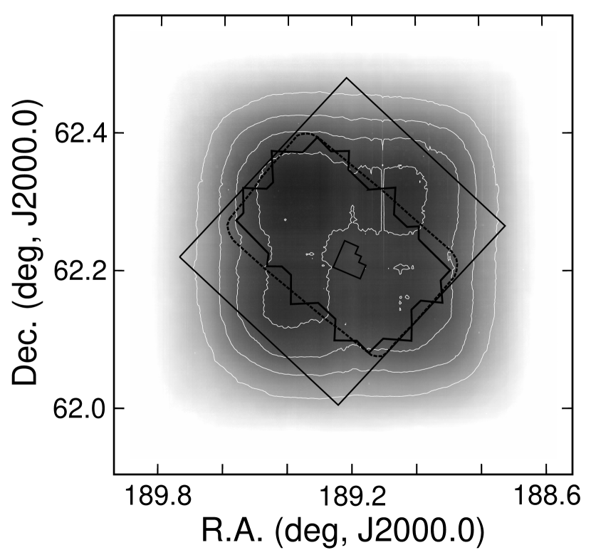
Figure 2.— Survey field layout. Grayscale shows the effective integration time of our WIRCam $K_{S}$ imaging. White contours show 80%, 60%, 40% and 20% of the maximum effective integration time. Black solid polygons show the GOODS-N ACS region and the HDF-N-proper. Black dashed contour shows the GOODS-N IRAC region. Black rectangle shows the Chandra Deep Field-North region.

Figure 3.— Cumulative area in the WIRCam $K_{S}$ image vs. effective integration time. The maximum effective integration time in the map is normalized to be 1.0. The effective integration time accounts for variation in efficiency of pixels, atmospheric extinction, and background brightness (see text). In shallow and intermediate depth regions where confusion is less important, noise very closely scales as inverse square-root of the effective integration time.

4. Reduction Quality

4.1. Astrometry

The SIMPLE reduction of the WIRCam $K_{S}$ image forced the positions of detected objects to match those in the astrometric catalog formed with the SDSS and the GOODS-N ACS catalogs. The resultant astrometry is excellently constrained by the ACS catalog in the central region and reasonably constrained by the SDSS catalog in the outer region. To quantify the (relative) astrometric accuracy, we selected well-detected compact sources (S/N $>20$ and FWHM $<1\farcs 2$) from the SExtractor catalog (Section 5). Nearly 4000 such sources have counterparts in the SDSS or GOODS-N ACS catalog. Figure 4 and Figure 5 show the offsets between the WIRCam and the SDSS/ACS positions. There are no observable systematic offsets between the WIRCam positions and both the SDSS and ACS catalogs. However, the astrometry is clearly better in the central part of the image where ACS sources were used to constrain the astrometric solution. The rms dispersions of the offsets are $0\farcs 05$ between WIRCam and ACS along both the R.A. and Dec. axes on nearly 4000 sources. The rms offsets between WIRCam and SDSS are larger, $0\farcs 08$ for RA and $0\farcs 10$ for Dec, on nearly 460 sources. We found that the SDSS and ACS catalogs have similar $\sim 0\farcs 1$ rms offsets between each other. This suggests the larger observed offsets between the WIRCam and SDSS positions may primarily be a consequence of an uncertainty internal to the SDSS catalog.

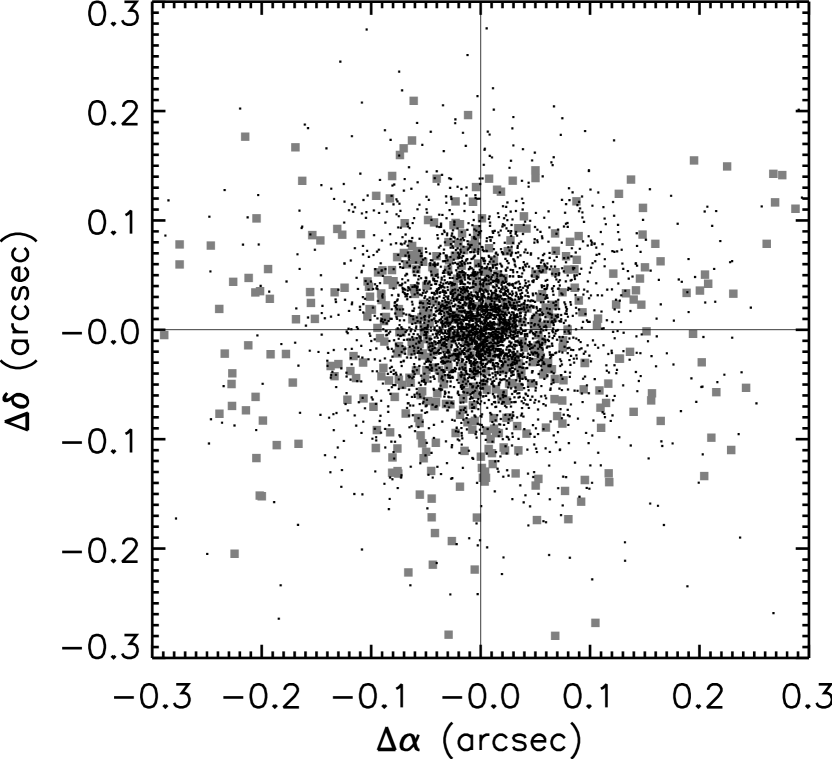
Figure 4.— Relative astrometric offsets between the WIRCam $K_{S}$ image and the SDSS and GOODS-N ACS catalogs. Approximately 4000 well-detected compact sources (S/N $>20$, FWHM $<1\farcs 2$) are plotted. Squares show the offsets of the WIRCam positions with respect to the SDSS positions, and dots show those with respect to the ACS positions.

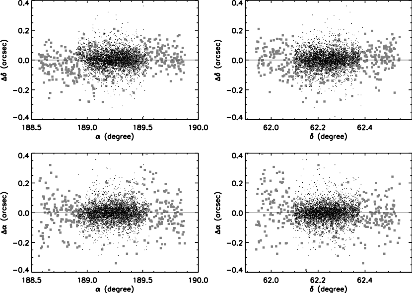
Figure 5.— Same as Figure 4, but as functions of RA and Dec.

The above measured rms offsets include both systematic and random errors. For example, the measured $0\farcs 05$ rms offset between WIRCam and ACS is slightly larger than the nominal positional uncertainty for FWHM $\sim 0\farcs 8$ and S/N $>20$, which should be $<0\farcs 04$. To estimate the systematic error in astrometry, we repeated the same measurements with higher S/N cuts and lower FWHM cuts. The rms offset decreases initially but stops decreasing when it approaches $0\farcs 03$, even when the selected sources have extremely high S/N (e.g., $>200$) and have FWHM comparable to the seeing. We conclude that there is an $\sim 0\farcs 03$ systematic uncertainty in our WIRCam astrometry in the GOODS-N ACS region. Such an error includes both the internal error in the ACS catalog and the error introduced by the image registration of SIMPLE. On the other hand, the rms offset between WIRCam and SDSS is $\sim 0\farcs 1$. Since all SDSS sources are detected in the WIRCam image with S/N $>100$ (median S/N is 2300), random noise is negligible here. We conclude that the systematic error is $\sim 0\farcs 1$ in outer regions where ACS positions are unavailable.

4.2. Photometry

The absolute flux scale of our WIRCam $K_{S}$ image was calibrated with 2MASS point sources in the image. Figure 6 shows the comparison between the 2MASS fluxes and the calibrated WIRCam fluxes derived with $5\arcsec$ diameter apertures. The ratio between the two is only flat in a narrow flux range. We chose $K_{s,AB}=14.44$–16.34 (the two vertical lines in Figure 6) for the calibration of the WIRCam image. Outside this range, there are nonlinearity problems with the WIRCam sensors (bright end) and selection effects in 2MASS (faint end). In the chosen range for calibration, the error-weighted mean of the flux ratios ($F_{\rm 2MASS}/F_{\rm WIRCam}$) for 70 sources is $1.0005\pm 0.5\%$, indicating that the overall absolute calibration of the WIRCam $K_{S}$ image is good to $\sim 0.5\%$. We note that the error bars in Figure 6 are dominated by 2MASS flux errors. Thus, the calibration of our WIRCam image is limited by the photometric quality of 2MASS. It is not possible to achieve better results unless we make frequent monitoring of standard stars during our observations, which is quite expensive in terms of observing time.

Figure 6.— Comparison of the 2MASS $K_{S}$ fluxes with the calibrated WIRCam $K_{S}$ fluxes. The noise in the WIRCam fluxes is plotted as horizontal error bars but is too small to be visible for the entire flux range and therefore makes a negligible contribution to the vertical error bars. This implies a calibration limited by the photometric quality of 2MASS. Vertical lines show the flux range used for the calibration. Sources outside the two lines are not used because of nonlinearity in WIRCam fluxes and selection effects in 2MASS. Within the two vertical lines, data that are $>3\sigma$ away from the mean are also excluded in the calibration.

We also investigated the photometric uniformity in our WIRCam $K_{S}$ image. The above value of 0.5% is the mean calibration error over the entire image. It is possible that the calibration of certain smaller regions is worse than this value. We subdivided the WIRCam image into four quadrants, roughly corresponding to data obtained from the four detector chips, and then compared the WIRCam fluxes with the 2MASS fluxes as we did for the entire image. For quadrants 1 through 4, the error-weighted flux ratios are $1.010\pm 0.9\%$ (16 sources), $-0.985\pm 0.9\%$ (19 sources), $1.009\pm 1.3\%$ (16 sources), and $1.011\pm 0.9\%$ (22 sources), respectively. In all of these cases, based on the numbers of available 2MASS sources and their 2MASS flux errors, the expected calibration errors are roughly 1%. The standard deviation of the four measured offsets is 1.3%, which compares well with the expected calibration error from 2MASS. This suggests that there is not an observable photometric gradient over size scales of $\sim 15\arcmin$. The absolute fluxes of objects are still limited by the photometric quality of 2MASS at this scale. The measured 1.3% variation is indeed excellent when compared to other $K$-band extragalactic deep surveys over similar size scales (e.g., 2% in the COSMOS survey, Capak et al., 2007).

5. $K_{S}$ Source Catalog

We used SExtractor (v2.5.0) to produce a $K_{S}$ source catalog. The most important source extraction parameters in SExtractor are summarized in Table 1. We provide our raw SExtractor $K_{S}$ catalog in this data release. We caution that the detection parameters (the first three in the table) that we adopted are somewhat aggressive in detecting faint sources, which may lead to more spurious sources (see § 5.2). The users of our data product may want to regenerate catalogs with more conservative values, based on the nature of their work.

Based on the raw catalog, we compiled a $K_{S}$ selected catalog, which is the primary product of this paper. We first estimated the true noise level in the WIRCam $K_{S}$ image. We masked the detected objects and convolved the image with circular kernels of amplitude 1.0 (i.e., flux apertures). The local (within $\sim 14\arcsec$) rms fluctuations in the convolved image were considered as errors in aperture photometry that include all possible sources of noise: photon noise, correlated noise between pixels, confusion noise from faint, undetected objects, and uncertainty in the estimate of the small-scale background. We compared the noise measured in this way with the photometric errors derived by SExtractor. We found that for all aperture sizes between $1\farcs 5$ and $5\arcsec$ in diameter, the ratio between the two errors is fairly insensitive to the aperture size and has a value of 1.28. Thus, we multiplied all of the flux errors in the SExtractor catalog by this factor to approximate the total noise. This does not affect the flux measurements.

Table 1SExtractor Parameters

Parameter	Value
DETECT_MINAREA	2
DETECT_THRESH	1.25
ANALYSIS_THRESH	1.25
FILTER	Y
FILTER_NAME	gauss_1.5_3x3.conv
DEBLEND_NTHRESH	64
DEBLEND_MINCONT	0.00001
CLEAN	Y
CLEAN_PARAM	0.1
SEEING_FWHM	0.8
BACK_SIZE	24
BACK_FILTERSIZE	6
BACK_TYPE	AUTO
BACKPHOTO_TYPE	LOCAL
BACKPHOTO_THICK	24
WEIGHT_TYPE	MAP_WEIGHT
WEIGHT_THRESH	10

The next step is to estimate aperture corrections. In our data reduction we calibrated the flux on 2MASS point sources using fixed $5\arcsec$ diameter apertures. Thus, SExtractor fluxes measured with $5\arcsec$ apertures do not need any aperture corrections and we consider $5\arcsec$ aperture fluxes to be the best estimate of the total fluxes of the sources. This clearly does not apply to the several most extended objects in the image, since their aperture corrections should be much larger than that for smaller objects (i.e., 2MASS point sources used in the calibration). Since they are not the major targets of our work, we did not attempt to obtain highly accurate fluxes for these very few sources.

Despite that $5\arcsec$ aperture fluxes are the best estimate of total fluxes, their S/N is relatively low. We thus looked for suitable fluxes measured with smaller apertures, and corrected the small aperture fluxes to $5\arcsec$ when it is necessary. We compared all other SExtractor flux options with the fixed $5\arcsec$ diameter aperture fluxes and found that the SExtractor “auto-aperture” fluxes agree excellently with them at all flux levels. In addition, the auto-aperture fluxes have the best optimized S/N for sources with various morphologies and fluxes. We thus decided to adopt directly the SExtractor auto-aperture fluxes and errors in our final catalog. We did not apply any additional corrections except for the aforementioned factor of 1.28 to the errors.

The adoption of SExtractor auto-aperture fluxes works excellently for nearly all sources. However, a very small number of sources (0.7% of total) are undetected in auto-apertures but detected in fixed apertures. For such sources, we adopted their $3\arcsec$ fluxes and corrected the fluxes to $5\arcsec$ with a median correction factor from all other detected sources. In addition, after all the above corrections to the fluxes and flux errors, some sources in the SExtractor raw catalog are still undetected. Given that our error estimate is realistic and the flux is well optimized, we considered sources with S/N $<1$ as undetected (1.9% of total) and only included their flux errors in the final catalog for upper limits. To keep the source number and order in our final $K_{S}$ catalog identical to those in the SExtractor raw catalog, we did not remove such undetected sources. This is for easy comparisons with the SExtractor catalog, in case the users of our data need to carry out more consistency or quality check.

We next evaluated the depth and completeness of our $K_{S}$ WIRCam catalog. In the central $30\arcmin\times 30\arcmin$ of the image where the sensitivity distribution is more uniform, the median 1$\sigma$ error among 3$\sigma$ sources is 0.15 $\mu$Jy, corresponding to a 3$\sigma$ limiting magnitude of 24.77. In the GOODS-N region, where the image is the deepest, the median 1$\sigma$ error is 0.12 $\mu$Jy, corresponding to a 3$\sigma$ limiting magnitude of 25.10. This is as deep as the IRAC 3.6 $\mu$m image in the same region.

5.1. Depth and Completeness

We estimated the completeness of our $K_{S}$ catalog with Monte Carlo simulations. We note that completeness is a complex function of flux, morphology, crowdedness, and source extraction. The results here are meant only to provide a guide. Exactly how one should carry out the completeness computation depends on the purpose of the study, and we shall leave this to the users of our data.

Here, we first randomly selected well-detected (S/N $>20$) sources from the SExtractor catalog. The selected sources span a wide range of flux, size, and shape. We extracted these sources from the WIRCam image and artificially dimmed or brightened them to the flux range of interest. Then we randomly placed them in the WIRCam image and ran SExtractor to detect them. Each time we only placed a small number of sources in the image so the overall source density did not change by $\gtrsim 1\%$. A total of $\sim 50,000$ sources were randomly placed in the image. The SExtractor catalogs for simulated images were processed identically to the real catalog. We considered a source recovered if it is detected at $>2\sigma$. We divided sources into four groups according to their half-light radii ($R_{h}$) and calculated the recovery rate in each 0.1 dex flux bin and $R_{h}$ group. The results in the central $30\arcmin\times 30\arcmin$ region are shown in Figure 7a. The 90% completeness limits for the two compact groups ($R_{h}\sim 0\farcs 47$ and $0\farcs 54$, comprising $>50\%$ of the total sample) are 1.10 $\mu$Jy ($7.3\sigma$) and 1.32 $\mu$Jy ($8.8\sigma$), respectively, equivalent to 23.80 and 23.60 magnitude. For the entire sample the mean 90% completeness weighted by the size distribution is 1.38 $\mu$Jy ($9.2\sigma$, which is equivalent to 23.55 magnitude. If we restrict this to the deeper 0.06 deg² GOODS-N IRAC region (Figure 7b), then the mean 90% completeness limit becomes 0.94 $\mu$Jy ($7.8\sigma$), or 23.96 magnitude.

Figure 7.— Completeness of the $K_{S}$ WIRCam catalog vs. flux and half-light radius in the central $30\arcmin\times 30\arcmin$ region (A) and in the GOODS-N IRAC region (B). Percentages given in the parentheses are fractions of objects in the four half-light radius groups in the $K_{S}$ catalog.

The above results show that the present WIRCam imaging is the deepest in the $K$-band over a substantial area. For example, the Very Large Telescope (VLT) NIR imaging in the GOODS-S is 90% complete at $K_{S}=23.8$ in a small area of $<10$ arcmin² (Grazian et al., 2006). On the other hand, our team (Wang, Barger, & Cowie, 2009) and Japanese groups (Kajisawa et al., 2006) have carried out extremely deep $K_{S}$ band imaging in the GOODS-N at the 8.2 m Subaru Telescope with a smaller $2048\times 2048\times 2$ imager. Kajisawa et al. (2009) combined all archived data to make a deep $K_{S}$ image of the GOODS-N. They achieved 3$\sigma$ limiting magnitudes of 25.5 and 26.5 in 103 arcmin² and 28 arcmin², respectively. This Subaru image is deeper than our WIRCam image (3$\sigma$ of 25.1 magnitude in the $\sim 200$ arcmin² GOODS-N region), but the area coverage is much smaller.

5.2. Spurious Sources

We took two approaches to estimate the spurious fraction, one based on an inverted image and the other based on multi-wavelength counterpart identification. First, we constructed an image with inverted background, and then ran through the same source detection and catalog compilation described above. This infers a spurious fraction of $\sim 20\%$ on sources with S/N $>3$, which is unreasonably high. After examining the image and the “sources,” we believe this is because the crosstalk of WIRCam produces negative holes near bright objects, making the noise non-Gaussian and greatly overestimating the spurious fraction. One evidence for this is that, in relatively crosstalk-free regions, the spurious fraction inferred from the inverted image dramatically decreases to $5\%$. This value of 5% is an upper limit since there are still low-level crosstalk effects.

We then looked for $K_{S}$ sources that are not detected in other images. In the region where the GOODS-N ACS and IRAC images overlap, there are 15112 $K_{S}$ sources detected at $3\sigma$. Among them, 489 (3.2%) sources do not have counterparts in the ACS catalog and are not detected at 3.6 and 4.5 $\mu$m at $3\sigma$ in the IRAC catalog described in the next section. (See § 7.1 for a slightly different comparison.) The fraction 3.2% is also an upper limit since we cannot rule out real $K_{S}$ sources being not detected in the ACS and IRAC images, especially given that the IRAC images are not substantially deeper than the $K_{S}$ image. This 3.2% upper limit is tighter than the 5% limit set by the inverted image, consistent with the above suggested non-Gaussian noise. Because of this limitation, it is difficult to further constrain the spurious fraction of our $K_{S}$ catalog. We suggest the users of our data to carry out independent source extraction if more conservative extractions are desired.

In Table 2 we summarize the basic properties of our WIRCam $K_{S}$ image described in this and previous sections.

Table 2Properties of the WIRCam Images

Properties	$K_{S}$ Image
Semesters	2006A, 2007A, 2008A
P.I.	L. Cowie, L. Simard
Total Integration	49.4 hr
Field Center (J2000.0)
R.A.	$189\arcdeg.227$
Dec.	$62\arcdeg.239$
Area ($T_{exp}>2$ hr)	0.25 deg2
Seeing FWHM	$0\farcs 8$
Calibration Uncertainty	1.3%
Astrometric Uncertainty	$0\farcs 03$–$0\farcs 1$
90% Completeness Limit	1.38 $\mu$Jy (23.55 mag.)
Spurious Fraction	$<3.2\%$

6. Colors in the WIRCam and IRAC Bands

We next used the WIRCam $K_{S}$ image and catalog as priors to analyze the fluxes of galaxies in the GOODS-N Spitzer IRAC images at 3.6–8.0 $\mu$m (M. Dickinson et al., in preparation). Similar work has been done previously. In both the GOODS-N (Laidler et al., 2007) and the GOODS-S (Grazian et al., 2006), ACS $z^{\prime}$-band images were used as priors to determine fluxes in the IRAC bands. While our $K_{S}$ image has a lower resolution than the ACS $z^{\prime}$ images, the waveband is much closer to the IRAC bands, making it a better choice for this type of analysis.

The primary goal is to better measure the colors of objects between the IRAC and $K_{S}$ bands. The nearly $2\arcsec$ resolution of IRAC is significantly worse than the typically sub-arcsecond resolution in the optical and NIR, but it is not much larger than the sizes of galaxies. This makes color measurements extremely uncertain. Normally one would need to sacrifice resolution in the optical and NIR bands to achieve this. The approach we describe below does not have this disadvantage. A secondary goal is to better separate IRAC fluxes of objects that are close to each other. There are nearly 20,000 $K_{S}$ detected source in the GOODS-N IRAC area, but SExtractor can only directly detect $11,000$ sources in the 3.6 $\mu$m IRAC image. One reason for the smaller number of sources in the IRAC image is that many objects are blended under the IRAC resolution. We will demonstrate that our method provides reasonable estimates of the IRAC fluxes of lightly blended objects.

6.1. Methodology

The basic idea is to convolve the $K_{S}$ image of each galaxy individually with a scaled convolution kernel to construct a model image for an IRAC image. The scaling of the kernel varies between galaxies because galaxies have different IRAC-to-$K_{S}$ flux ratios (i.e., colors). The set of scaling factors that produce the best model image are then the best estimates of the flux ratios.

It is immediately obvious that the results would be sensitive to the evaluation of whether a model best approximates the IRAC image, as well as whether the chosen convolution kernel well represents the PSF. In Laidler et al. (2007) and Grazian et al. (2006), the model that produced the minimum $\chi^{2}$ was considered as the best model. In such analyses, $\chi^{2}$ is very sensitive to the mismatch of the PSF, and unfortunately, there is a huge uncertainty in the PSFs in the IRAC bands. This was pointed out by Grazian et al. and is also clearly shown in Figure 8. It is thus unclear to us whether or not $\chi^{2}$ analyses are the best approach. Here we present an alternative approach based on the widely used image deconvolution technique in radio astronomy—CLEAN (Högbom, 1974). Instead of minimizing the $\chi^{2}$ of the pixels, CLEAN determines the scaling of the kernels based on the fluxes of the image components. This is very attractive to us since our true goal is to be able to account for the fluxes detected in the IRAC images. As long as the fluxes in an IRAC image can be cleanly removed by subtracting a model, we consider the model to be the best. Below we describe the basic steps in our analysis of the galaxy colors. We hereafter refer to our technique as REALCLEAN, since it is done in real space instead of Fourier space.

6.1.1 PSF Construction

The GOODS-N IRAC images have pixel scales of $0\farcs 6$, so we background subtracted and resampled them to the WIRCam $0\farcs 3$ pixel scale. During the resampling, the IRAC images were also slightly warped such that the positions of objects precisely match those in the WIRCam image. To construct PSFs for the IRAC and WIRCam images, we selected $\sim 20$ bright but unsaturated, point-like, and isolated objects in these images. The images of these objects were aligned, stacked, and normalized to form the PSFs. The IRAC PSFs were then deconvolved by the WIRCam PSF with a maximum likelihood deconvolution of a few iterations. The deconvolved IRAC PSFs were used as the convolution kernels to convolve the WIRCam image. One may worry about the uncertainty in the deconvolution of the PSFs. We also tried an alternative approach that does not require the deconvolution of the IRAC PSF, in which we measured colors in the IRAC images that are convolved with the WIRCam PSF and in the $K_{S}$ image that are convolved with the IRAC PSFs (see § 6.4). We did not see a systematic difference between the two approaches. We thus adopted the deconvolved IRAC PSFs as the convolution kernels.

6.1.2 Object Identification

In the background-subtracted WIRCam $K_{S}$ image, for each detected object we identified pixels associated with that object. This was done with the “segmentation map” provided by SExtractor. This allowed us to apply different scaling factors to the convolution kernels on different objects. A minor drawback here is that very faint pixels in the outer parts of galaxies would be missed. However, as long as these faint pixels do not have dramatically different colors from the brighter cores of the galaxies, our measured colors can still be considered as good estimates of the flux-weighted mean colors of galaxies. Another minor drawback is pixels that contain emission from more than one object. This would only become problematic when objects are not well resolved in the WIRCam image. Since this is the fundamental limit of the WIRCam observations, we did not attempt to resolve this issue.

6.1.3 REALCLEANing Bright Objects

To obtain model images that best approximate the observed IRAC images, we use our REALCLEAN method, which is especially useful when determining fluxes of blended galaxies. In a REALCLEAN cycle, we first identify the brightest galaxy in the IRAC image. Then we remove a small fraction (25% at 3.6 $\mu$m down to 10% at 8.0 $\mu$m; this factor is often called the “gain”) of its flux from the IRAC image by subtracting a model image constructed by convolving the WIRCam image with the above mentioned kernel. The flux is determined by placing a circular aperture at the object. We used aperture diameters of $4\arcsec$, $4\arcsec$, $5\arcsec$, and $6\arcsec$ for the IRAC 3.6, 4.5, 5.8 and 8.0 $\mu$m bands, respectively. Despite the fact that such aperture photometry is affected by nearby objects, because we only look at the brightest object and because the gain is $\ll 1$, we guarantee that we do not over-subtract the object. To speed up the REALCLEAN process, we subtract fractional fluxes from many objects in one REALCLEAN cycle. However, in each REALCLEAN cycle we only subtract objects that are sufficiently far away from each other that locally each subtracted object is the brightest. In the subsequent REALCLEAN cycle we look for the next brightest objects in the subtracted image and subtract small fractions of fluxes from them. We repeat this iterative procedure until no objects in the residual IRAC image have fluxes brighter than a few $\sigma$.

It is interesting to note that the above procedure is similar to the CLEAN deconvolution of radio interferometric data (see a summary in Cornwell, Braun, & Briggs 1999) in many ways. To limit the degrees of freedom, CLEAN is often limited to CLEAN windows or boxes within which emission is known or guessed to be present. CLEAN also sometimes uses priors to improve the speed of convergence of the solution. These are exactly what our procedures do: we only subtract IRAC fluxes at the locations of $K_{S}$ detected galaxies, and we use the WIRCam $K_{S}$ images of the galaxies as the model.

6.1.4 Final Residual Flux Minimization

Once REALCLEAN reaches a few $\sigma$, all objects have similar brightness and REALCLEAN is no longer efficient and necessary. Thus, we measured the residual IRAC fluxes of all of the WIRCam objects and subtracted them from the IRAC image all at once. This global subtraction unavoidably over-subtracts blended objects, especially those whose separations are less than the flux aperture sizes. Since the global subtraction is carried out only after the objects are REALCLEANed to a few $\sigma$, the amount of over-subtraction is small. Nevertheless, the over-subtraction can be further minimized.

We estimated the over-subtraction by measuring the fluxes again in the residual image. Then we re-iterated the global subtraction by adjusting the subtracted fluxes and again measured the over-subtraction in the next residual image. In each iteration, the adjustment of fluxes were small fractions (equal to the REALCLEAN gains) of the estimated over-subtraction. This slowly brought the residual fluxes of galaxies in the subtracted image from negative (after the first global subtraction following the REALCLEAN cycles) to nearly zero after tens of iterations. In the iterations, we closely watched the residual fluxes of galaxies to see if they converged to zero. When the residual fluxes no longer converged (typically after 40–60 iterations), we stopped the iterations. Fluxes subtracted in the REALCLEAN stage and in this minimization stage were added to make the total IRAC fluxes of the WIRCam $K_{S}$ detected galaxies.

For each IRAC band, there are two epochs of observations covering different areas in the GOODS-N but with some overlap. All the procedures described above, including the PSF construction, were carried out independently on each single-epoch image. This is because the two epochs have different orientations of pixels and PSFs. For sources in the overlap region, we adopted the error weighted fluxes from the two epochs.

6.1.5 Flux and Error Measurements

As mentioned, we used $4\arcsec$–$6\arcsec$ diameter apertures to measure fluxes, or in other words, to evaluate whether the model best removes fluxes of galaxies. Such small aperture sizes nicely cover the cores of the IRAC PSFs and minimize influences from nearby sources. We also derived aperture corrections from the convolution kernels. However, the proper correction is a function of the sizes of the galaxies, which are not exactly point sources under the IRAC resolution. This biases the measured fluxes, especially when the apertures are small. Our small apertures also miss the information in the outer wings of the PSFs. To account for these, we repeated the REALCLEAN procedures with 50% larger apertures and compared the results with those from small-aperture REALCLEANs. Such aperture sizes are comparable to the sizes of the first diffraction rings in the IRAC PSF and are sufficiently large for the majority of galaxies in the GOODS-N. We applied a constant correction factor (2%–6%) to all the small-aperture fluxes, derived from the large-aperture REALCLEAN on high S/N and isolated sources.

We estimated flux errors in a similar way to those for the WIRCam fluxes described in § 5. We convolved the residual IRAC images with circular uniform kernels of amplitude 1.0 and measured the rms fluctuation locally. This way, the measured noise included not only photon noise, confusion noise, and correlated noise, but also rough estimates of the uncertainties caused by imperfect object removal in the entire REALCLEAN and flux minimization processes. IRAC fluxes and errors measured in this way are included in the $K_{S}$ selected source catalog in this data release (Table 3).

6.2. Quality and Performance

6.2.1 Residual Images

To evaluate the performance of the above REALCLEAN-based procedures, we first visually inspected the residual images after subtracting the best models. Figure 8 shows the HDF-N region of the IRAC images before and after the subtraction. Overall, the subtraction of IRAC objects with our REALCLEAN method appears reasonably good in all IRAC channels. However, minor residual effects can be seen. There are faint halos around many objects in all channels after the subtraction, likely a consequence of the fact that our small flux apertures did not fully account for fluxes from slightly extended objects. On the other hand, on compact objects there are residual patterns around the cores of the objects. In the first two IRAC channels, this indicates a $\sim 5\%$ uncertainty in the adopted IRAC PSF. Because this occurs across the entire field, this is unlikely to be an effect of PSF variation or position-dependent mis-registration. This is the most severe in the first two IRAC channels, suggesting that under-sampling of the PSF by the large IRAC pixels may have played a role. However, the exact reason remains unclear to us. The 5.8 $\mu$m channel has the cleanest subtraction of IRAC objects. It gets slightly worse again in the 8.0 $\mu$m channel, likely because the 8.0 $\mu$m morphology becomes sufficiently different than that in the $K_{S}$-band.

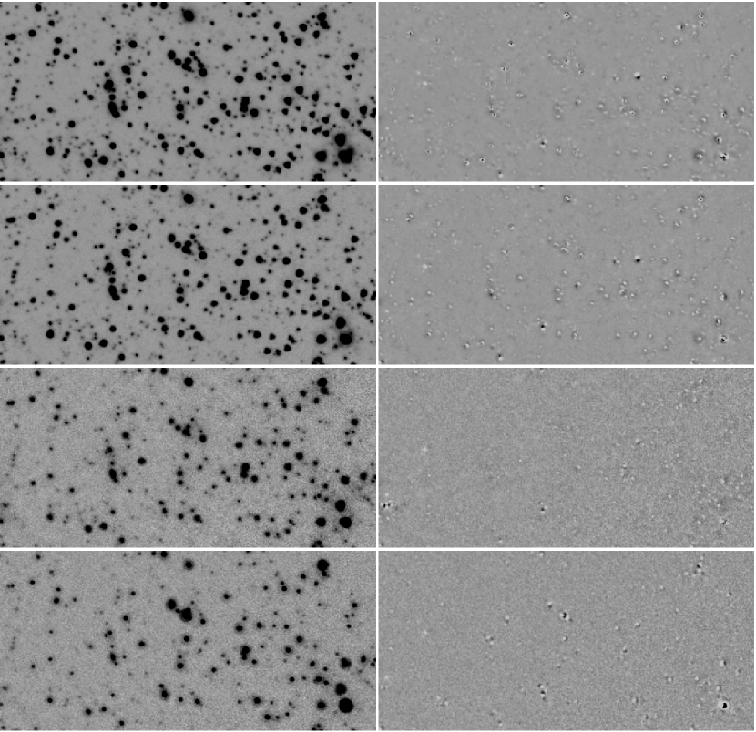
Figure 8.— Results of the REALCLEAN subtraction and residual flux minimization. Images to the left are the original IRAC images in the HDF-N. Images to the right are the residual images after subtracting all sources with minimal residual fluxes. From top are the IRAC images at 3.6, 4.5, 5.8 and 8.0 $\mu$m. Each residual image is shown with a brightness scale identical to its original image. All images are shown with inverted scales.

Figure 9.— Simple Monte Carlo simulations of REALCLEAN on two blended objects. Four large panels show results from the four IRAC channels. The simulations include various flux ratios and angular separations for the blended pairs. Results of different flux ratios (FR) are shown in the sub-panels. Vertical axes show the output-to-input flux ratios of the fainter objects between the blended pairs. Error bars show the dispersion among various realizations. Note that the 8.0 $\mu$m panel has a different vertical scale. The lack of data points in some regions of the plots means that even the SExtractor cannot separate the blended sources in the WIRCam images. REALCLEAN cannot deal with such cases since it is based on the SExtractor WIRCam catalogs.

6.2.2 Monte Carlo Simulations

The above visual inspection of the residual images qualitatively shows that overall our REALCLEAN approach can account for the IRAC fluxes of $K_{S}$-band detected objects and that there are no catastrophic failures in subtracting off the IRAC objects. However, this does not guarantee that fluxes are correctly assigned to objects when multiple objects are blended by the IRAC PSF. To test this, we carried out simple Monte Carlo simulations.

We simulated objects of high S/N ($\sim 20$) blended by nearby objects. The flux ratios between the blending bright sources and the targets are from 1.0 to 100. The separations between the targets and the nearby sources are from $1\farcs 3$ to $4\arcsec$, with various position angles. All objects are point-like and have flat spectra. PSFs derived from the two epochs of the real IRAC images and the real WIRCam image were used to create the associated simulated images. All the images were processed identically to the above REALCLEAN and catalog making procedures.

We shown the results of the simulations in Figure 9. A few trends can be observed and are indeed as expected. REALCLEAN performs the best when the fluxes ratios are $<10$ and separations are $\gtrsim 2\arcsec$. At very small separations of $1\farcs 3$, REALCLEAN can also correctly recover the fluxes if the nearby objects are less than $2\times$ brighter then the targets. Among the $\sim 15000$ real sources detected at 3.6 $\mu$m in our final catalog (§ 6.3), 90% of their brightest neighbors fall in the above ranges of flux ratio and angular separation.

There no data points in regions of large flux ratios and small separations (including flux ratios of greater than 31.6, which are not shown). These are the cases in which even SExtractor cannot resolve the blended sources in the WIRCam images. REALCLEAN cannot determine the IRAC fluxes if the sources are not resolved by SExtractor in the WIRCam images. At the boundary when the SExtractor can barely resolve the blended pairs, REALCLEAN either over-estimates (large separation) or under-estimates (small separation) the fluxes of the targets. The amount of over and under-estimate can be up to 40%. Here we are pushing the limits of both REALCLEAN and SExtractor. In our catalog, the fractions of sources with $<4\arcsec$ neighbors that are $>17.8\times$ and $>31.6\times$ brighter are 5.7% and 3.6%, respectively.

The above results imply good REALCLEAN fluxes for the majority of sources in our catalog. A small number of sources may have IRAC fluxes affected by very bright neighbors. The effect is generally not $\gg 40\%$ before SExtractor becomes unable to detect the faint sources. The caveat here is that the above simulations are very simple. One may conduct much larger simulations with variable object morphology, S/N level, and number of blended sources. We do not think these are particularly useful given the large uncertainty in the IRAC PSF discussed in § 6.2.1. Realistic simulations should take into account such uncertainties, folding in how the PSF is under-sampled by the IRAC pixels and how the observations were carried out and reduced to better sample the images (e.g., dither and drizzle), which is out of the scope of this paper. Without good knowledge about the PSF, going further beyond the above simulations does not likely help on understanding the performance of REALCLEAN. In what follows, we will rely on simple consistency checks within the available data, paying special attention to blended galaxies.

6.2.3 Overlap Region Between Epochs 1 and 2

The GOODS-N IRAC observations consist of data from two epochs. Both the PSFs and the pixels in these two epochs have different orientations. The two epochs of imaging overlap in approximately 35 arcmin² of area at the center of the GOODS-N. Since we ran our REALCLEAN procedures on the two epochs separately, we compared our results in the overlap region to see if they are consistent. Figure 10 shows the ratios of the fluxes derived from epochs 1 and 2. The dashed curves in each plot show the dispersion of the flux ratios, and the solid curves show the expected dispersion based on flux errors estimated in § 6.1.5. The fact that the two curves are very close to each other is a strong indication that our error estimate is realistic and that the uncertainty of the fluxes derived from our REALCLEAN procedure is limited by the noise in the data.

We examined the IRAC sources that have nearby $K_{S}$-band detected objects with separations of $1\arcsec$–$2\arcsec$ (diamonds and $2\arcsec$–$3\arcsec$ (triangles). In the $1\arcsec$–$2\arcsec$ category, the distributions of the flux ratios are not significantly different from the main sample, except that at 8.0 $\mu$m. At 8.0 $\mu$m the $2\arcsec$–$3\arcsec$ category has a distribution similar to the main sample. These results suggest that our procedures produce consistent results against slight changes in the PSF for blended sources with separations greater than $1\arcsec$ at 3.6, 4.5, and 5.8 $\mu$m and $2\arcsec$ at 8.0 $\mu$m. In the $K_{S}$ catalog for sources with S/N $>5$, the median separation between galaxies and their nearest neighbors is $4\farcs 1$, and 99.5% of sources do not have a nearest neighbor within $1\arcsec$. This suggests that nearly all of the fluxes we derived for the first three IRAC channels are reliable. On the other hand, among the $\sim 5000$ 8.0 $\mu$m detected sources, approximately 10% of the sources have nearest neighbors at $<2\arcsec$. Their fluxes are more problematic, if Figure 10 is indicative. However, the percentage would be lower if we only considered sources whose nearest neighbors were significantly brighter than themselves. One can imagine that if sources with similar fluxes are blended, REALCLEAN naturally assigns similar fluxes to both if the gain is sufficiently small (which is the case for our 8.0 $\mu$m REALCLEAN). On the other hand, if sources with different fluxes are blended, the procedure might fail, especially on the fainter member of the pair. These are also indicated in our Monte Carlo simulations.

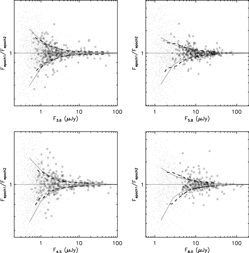
Figure 10.— Comparison of the IRAC fluxes derived from the two epochs. Dots show the full sample. Diamonds and triangles show galaxies whose nearest $K_{S}$ neighbors have angular separations of $1\arcsec$–$2\arcsec$ and $2\arcsec$–$3\arcsec$, respectively. Dashed curves show the dispersion of the full-sample data. Solid curves show the expected dispersion based on flux uncertainties derived in § 6.1.5. The $y$-axes have logarithmic scales.

Figure 11.— IRAC and $K_{S}$-band colors vs. redshift for spectroscopically identified galaxies. Only galaxies with S/N $>10$ at each waveband are plotted (dots). Diamonds show galaxies whose nearest neighbors are within $1\arcsec$–$2\arcsec$. X-marks show X-ray selected AGNs (hard or soft X-ray luminosities greater than $10^{42}$ erg s^-1). Solid curves show unreddened galaxy templates of, from red to blue, M 82 (a dusty starburst), M 100 (a spiral), and a dustless starburst. Dotted curves show the M 82 template with $A_{V}=2.0$.

6.2.4 Comparison with SED Models

The key goal of our analyses is to obtain accurate colors for the WIRCam and IRAC sources. We selected sources that have redshifts in the spectroscopic survey of B08 and compared their colors with model SEDs. Here we used two SEDs with dust and polycyclic aromatic hydrocarbon (PAH) features from Silva et al. (1998), M 82 (a dusty starburst) and M 100 (a spiral), and a dustless starburst template from Kinney et al. (1996) that has a blue stellar continuum and strong recombination lines. We also reddened the M 82 SED with $A_{V}=2.0$ using the Calzetti et al. (2000) extinction law. These four SEDs represent a broad range of galaxy colors. Figure 11 shows the comparison between the data and the model SEDs. As in Figure 10, galaxies with nearest neighbors of $1\arcsec$–$2\arcsec$ separations are shown with diamonds.

Overall the derived IRAC and $K_{S}$ colors match the SED models excellently. At $z\sim 2.2$ and 3.4 in the $F_{3.6}/F_{Ks}$ ratio and $z\sim 3$ in the $F_{4.5}/F_{3.6}$ ratio, there are substantial numbers of observed colors significantly bluer than the starburst model. This is true for both isolated galaxies and galaxies with close neighbors. We believe these blue “outliers” are not artifacts of our REALCLEAN procedures but rather objects with emission lines even stronger than those in the starburst template. The lines are likely H$\alpha$ and [S II] (entering $K_{S}$ at $z\sim 2.2$), H$\beta$ and [O III] (entering $K_{S}$ at $z\sim 3.4$), and [S III] (entering the 3.6 $\mu$m band at $z\sim 3$), all present in the starburst template. We attempted to verify this with our spectroscopic data. Unfortunately, we only have optical spectra on three of these galaxies, as most of the redshifts are adopted from Reddy et al. (2006). The three sources have standard Lyman break galaxy spectra with strong C IV absorption. In one case there is also Ly$\alpha$ emission. In the other cases we do not cover Ly$\alpha$. Galaxies with strong rest-frame optical (corresponding to $K_{S}$ and IRAC bands at these redshifts) emission lines have absorption lines in the rest-frame ultraviolet (corresponding to optical at these redshifts). Given their rest-frame ultraviolet continua, these three galaxies are inevitably strong emission-line galaxies in the rest-frame optical. This is consistent with strong emission lines causing the blue observed colors at $K_{S}$ and IRAC.

There are a few unexplained blue outliers at $z\sim 1.4$–2 in $F_{3.6}/F_{Ks}$ and at $z\sim 2$ in $F_{4.5}/F_{3.6}$. They might be fluxes mistakenly assigned by our REALCLEAN procedure. However, if this is the case, it would be very surprising if such outliers are not observed at all at $z<1.5$, where most of the spectroscopic samples lie. An alternative explanation is that they are galaxies with misidentified redshifts. We have spectra for these galaxies, except for two whose redshifts were adopted from Reddy et al. (2006). We inspected the available spectra and did not see obvious signs of misidentification. Thus, the nature of these blue outliers remains unclear. Nevertheless, we emphasize that the observed IRAC colors of the majority of the galaxies match excellently with the models at nearly all redshifts. Combining this with our observations in § 6.2.3, we are confident that our REALCLEAN procedures correctly assigned fluxes to nearly all of the IRAC sources.

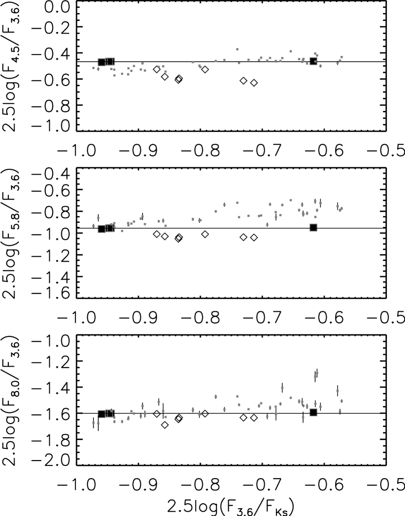
Figure 12.— IRAC colors of spectroscopically identified stars (dots) and IRAC primary absolute calibrators. A-type calibrators are shown as filled squares and K-type calibrators are shown as open diamonds. The mean colors of the four A-type calibrators are shown with horizontal lines.

6.2.5 Calibration

The last performance test is a comparison with Spitzer absolute flux calibrators in Reach et al. (2005). Figure 12 shows the measured colors of the spectroscopically identified stars brighter than $K_{S}=19$ and the colors of the IRAC primary absolute calibrators in Reach et al. Among the calibrators, A dwarfs are shown with filled squares and K giants are shown with open diamonds. Reach et al. found a displacement between the calibration derived from A and K stars, especially in the first two IRAC channels. The reason for this is unclear and the authors decided to adopt an absolute calibration based on only A stars. In Figure 12 we see a gradual drift of the IRAC colors for our data with respect to the IRAC calibrators, from blue to red in the $F_{3.6}/F_{Ks}$ color. However, since the IRAC absolute calibration is based on A stars, it is more appropriate for us to compare A stars only. At the very blue end where we find three of the four A-type IRAC calibrators, our observed colors for the stars agree excellently with the IRAC calibrators. The largest offset is observed in the $F_{4.5}/F_{3.6}$ color (top panel), where the stars in the left appear to be $\sim 0.05$ magnitude bluer than the mean color of the A-type calibrators (measured from stars with $x$-axis values $<-0.9$). We thus conclude that our colors are well calibrated, with systematic errors no larger than $\sim 5\%$.

6.2.6 Known Issues

Despite all the tests above, the IRAC fluxes derived by our REALCLEAN procedures are not perfect. The PSFs we used for REALCLEAN can only effectively remove fluxes within $\sim 4\times$ the FWHM. There are about 10 or so very bright stars with PSF wings, which are much broader than this. Objects close to these bright stars, especially those on the diffraction spikes and crosstalk features, have systematically higher IRAC fluxes. A more subtle effect is seen in a few very crowded regions where more than three objects heavily overlap. In such configurations objects that are close to the centers of the groups of objects can have systematically higher fluxes. Visual inspections identify only a handful of such examples in each IRAC band.

Table 3$K_{S}$ Selected Multi-Band Catalog

ID	R.A.	Dec.	$F_{Ks}$	$\sigma_{Ks}$	$F_{3.6}$	$\sigma_{3.6}$	$F_{4.5}$	$\sigma_{4.5}$	$F_{5.8}$	$\sigma_{5.8}$	$F_{8.0}$	$\sigma_{8.0}$
	(J2000.0)	(J2000.0)	($\mu$Jy)
54739	189.104027	62.278061	6032.930	0.229	2741.866	0.936	1662.465	0.632	1160.937	1.426	611.762	0.790
54740	189.054105	62.283076	94.032	0.235	82.640	0.158	53.823	0.203	56.101	0.860	38.938	0.841
54741	188.919686	62.287091	0.286	0.066	0.000	0.000	0.000	0.000	0.000	0.000	0.000	0.000
54742	189.482580	62.282344	54.345	0.233	31.454	0.173	23.463	0.171	17.371	0.468	9.386	0.356
54743	189.139434	62.284211	35.129	0.165	21.971	0.136	16.208	0.214	13.119	0.402	6.451	0.718
54744	188.774407	62.286231	1.029	0.213	0.000	0.000	0.000	0.000	0.000	0.000	0.000	0.000
54745	189.178137	62.286029	2.824	0.173	2.823	0.110	2.159	0.130	2.149	0.361	2.311	0.507
54746	189.747513	62.286519	0.184	0.075	0.000	0.000	0.000	0.000	0.000	0.000	0.000	0.000
54747	188.729697	62.286591	0.335	0.142	0.000	0.000	0.000	0.000	0.000	0.000	0.000	0.000
54748	189.369137	62.286251	2.069	0.103	2.484	0.121	1.975	0.133	1.891	0.432	1.085	0.262
54749	189.193693	62.286347	0.830	0.117	0.985	0.043	0.762	0.051	0.000	0.303	0.000	0.000
54750	189.071498	62.286398	1.692	0.110	2.196	0.094	1.674	0.117	0.894	0.353	0.752	0.254

Note. — Table 3 is published in its entirety in the electronic edition of the Astrophysical Journal. A portion is shown here for guidance regarding its form and content. If the measured fluxes are less than the flux errors (S/N $<1$), zeros are assigned to the fluxes but the errors are given for upper limits. Zero flux errors mean that the sources do not have measurements (i.e., the $K_{S}$ sources are not in the IRAC regions).

6.3. Combined NIR and IRAC Catalog

We combined the IRAC fluxes derived with the REALCLEAN procedures with the $K_{S}$ source catalog to form the final multiband catalog. The catalog is presented in Table 3. The total number of sources is identical to the SExtractor $K_{S}$ catalog, but not every $K_{S}$ source contained a detection in the IRAC bands. As is the case for the $K_{S}$ fluxes, our IRAC flux errors are quite realistic (see § 6.2.3 and Figure 11), and we consider the IRAC sources with S/N $<1$ to be undetected. Table 4 summarizes the number of detections and upper limits in the multiband catalog.

We have searched for missing sources in the REALCLEANed IRAC images. There may exist sources that are so red that they are detected in the IRAC channels but not in the $K_{S}$ image. These sources are mostly too faint to be detected in the WIRCam $K_{S}$ image. A small fraction of them are blended with nearby sources in the $K_{S}$ image and not extracted by SExtractor. To search for such sources, we combined the REALCLEANed (those in the right hand side of Figure 8) 3.6 and 4.5 $\mu$m IRAC images and masked the $K_{S}$ detected objects. This naturally excludes sources that are too close to bright objects. We visually inspected the REALCLEANed images and look for rermaining sources there. We excluded sources that are likely cosmic rays in the IRAC images, or other kinds of artifacts. We also examined the 5.6 and 8.0 $\mu$m REALCLEANed images, and we found that all the sources seen in these two images can be extracted from the 3.6+4.5 $\mu$m REALCLEANed images. Thus, the positions of such sources were measured in the 3.6+4.5 $\mu$m image and their fluxes were measured in all the individual IRAC images. The $K_{S}$-band fluxes and flux errors are measured in the same way as described in § 5. The positions, $K_{S}$ fluxes, and IRAC fluxes of a total of 358 such sources are listed in Table 5. All of them have detections in at least two IRAC bands, and 112 of them are detected in all four bands. As can be seen in Figure 8, source extractions in the REALCLEANed images are difficult and can be severely affected by the imperfect source subtraction described in § 6.2.1. We warn the readers that Table 5 is very likely an incomplete list of $K_{S}$-faint IRAC sources.

Table 4Number of Sources and Detection Limits in the Multi-Band Catalog

Waveband	Total Number	Detections	Upper Limits	Depth ($\mu$Jy)
$K_{S}$	94951	75187	1784	0.18
3.6 $\mu$m	16950	15018	731	0.11
4.5 $\mu$m	16631	14015	1000	0.12
5.8 $\mu$m	16870	8481	4551	0.42
8.0 $\mu$m	15184	7245	4118	0.42

Note. — The total number column gives the number of IRAC flux measurements at the locations of the $K_{S}$ objects. They are mainly determined by the area coverage of the IRAC images. Detections are measurements with $>3\sigma$ fluxes. Upper limits are measurements with $<1\sigma$ fluxes. Depths are median 1$\sigma$ errors among sources detected at 3$\sigma$ for the entire maps.

Table 5IRAC Sources without $K_{S}$ Counterparts

R.A.	Dec.	$F_{Ks}$	$\sigma_{Ks}$	$F_{3.6}$	$\sigma_{3.6}$	$F_{4.5}$	$\sigma_{4.5}$	$F_{5.8}$	$\sigma_{5.8}$	$F_{8.0}$	$\sigma_{8.0}$
(J2000.0)	(J2000.0)	($\mu$Jy)
189.049062	62.133903	0.227	0.091	0.945	0.128	0.894	0.160	1.597	0.625	1.049	0.385
189.086443	62.134109	0.000	0.108	0.400	0.127	0.480	0.151	0.000	0.247	0.000	0.614
189.049452	62.138386	0.000	0.074	0.377	0.078	0.110	0.080	1.870	0.560	0.741	0.377
189.209527	62.140676	0.000	0.114	0.908	0.181	1.037	0.191	1.419	0.731	1.270	0.541
189.215522	62.144264	0.000	0.094	0.638	0.212	1.049	0.190	0.000	0.284	1.507	0.590
189.241636	62.145789	0.250	0.082	0.423	0.169	0.589	0.118	0.590	0.402	0.000	0.282
189.246272	62.146429	0.217	0.105	0.468	0.151	0.623	0.122	0.377	0.324	0.000	0.258
189.087076	62.150220	0.000	0.087	0.756	0.232	0.366	0.211	0.696	0.300	0.000	0.425
188.998232	62.150675	0.000	0.095	0.269	0.117	0.581	0.159	0.000	0.337	0.426	0.335
189.018589	62.153052	0.192	0.101	0.345	0.112	0.277	0.129	0.000	0.496	0.769	0.557
189.045539	62.154243	0.000	0.093	0.572	0.129	0.511	0.146	1.249	0.549	0.000	0.438
188.981101	62.154402	0.254	0.081	1.280	0.198	2.046	0.210	3.184	0.922	2.433	1.231

Note. — Table 5 is published in its entirety in the electronic edition of the Astrophysical Journal. A portion is shown here for guidance regarding its form and content. If the measured fluxes are less than the flux errors (S/N $<1$), then zeros are assigned to the fluxes, but the errors are given for upper limits.

Figure 13.— Comparison between the colors derived with the XCONV and REALCLEAN methods. All sources in both catalogs are plotted.

Table 6$K_{S}$-to-IRAC Colors Derived with Cross-Convolution

ID	$K_{S}-3.6$$\mu$m	$K_{S}-4.5$$\mu$m	$K_{S}-5.8$$\mu$m	$K_{S}-8.0$$\mu$m
54739	-0.839	-1.434	-1.807	-2.430
54740	-0.135	-0.628	-0.576	-0.884
54741	99.000	99.000	99.000	99.000
54742	-0.579	-0.928	-1.283	-1.879
54743	-0.517	-0.862	-1.095	-1.537
54744	99.000	99.000	99.000	99.000
54745	0.154	-0.067	0.166	0.174
54746	99.000	99.000	99.000	99.000
54747	99.000	99.000	99.000	99.000
54748	0.365	0.190	-0.273	-0.473
54749	-0.659	-0.817	99.000	99.000
54750	0.283	-0.006	-0.249	-0.316

Note. — Table 6 is published in its entirety in the electronic edition of the Astrophysical Journal. A portion (identical to that for Table 3) is shown here for guidance regarding its form and content. Source ID and the total number of sources are both identical to that in Table 3. All colors are in the AB magnitude system. Sources with no measurements are assigned 99.0.

6.4. Alternative Color Measurements with Cross-Convolution

In the previous subsections, we described our REALCLEAN method of obtaining robust color measurements, for overcoming the issues of the very different PSFs and the blending of sources. Here we describe an alternative method that can better handle the former issue but is more vulnerable to the latter. We started with the background subtracted and registered images used for the REALCLEAN procedure. For each single-epoch IRAC image, we convolved the WIRCam $K_{S}$ image with the IRAC PSF and the IRAC image with the WIRCam PSF. We refer to this procedure as cross-convolution (XCONV). We then used the 2-image mode of SExtractor to detect sources in the unconvolved WIRCam image and to measure the WIRCam and IRAC fluxes in the XCONVed images at the locations of the detected WIRCam sources. The PSFs in the XCONVed images have FWHMs of slightly larger than $2\arcsec$. After experimenting with various photometry apertures, we found that a $3\arcsec$ aperture gives the best compromise for S/N, inclusion of most fluxes from a wide range of source structure, and blending of sources. Here we focus on the $K_{S}$-to-IRAC colors measured this way, and we do not attempt to measure total fluxes.

The advantage of the XCONV method is clear: the PSFs are ideally matched and deconvolution of the IRAC PSFs is not required (unlike in the REALCLEAN method). The disadvantage is the severely degraded $K_{S}$ image resolution, which prevents the extraction of information on both blended sources and faint sources. Because of these, we consider the XCONV colors of relatively bright and isolated sources to be more robust than the REALCLEAN colors. However, as shown in Figure 13, the XCONV colors and the REALCLEAN colors turn out to be remarkably consistent. The systematic offsets in Figure 13 between these two colors for $\sim 1800$ $F_{K_{S}}>10$ $\mu$Jy objects are 0.002, -0.024, 0.031, and 0.030 (from 3.6 to 8.0 $\mu$m). We examined the small number of objects in the figure that have offsets of $>0.05$ at $F_{K_{S}}>10$ $\mu$Jy. They are either close to bright objects (a weakness of the XCONV method) or are in regions with multiple intermediate brightness objects (a weakness of the REALCLEAN method, as mentioned in § 6.2.6).

The excellent consistency between the XCONV colors and the REALCLEAN colors further shows that our REALCLEAN method is robust. We thus consider the REALCLEAN catalog as the primary product of this work, and we recommend it for most applications. On the other hand, since the XCONV colors have unique advantages in their own right, we also provide the XCONV colors in Table 6. We remind the reader that the XCONV colors are less reliable on faint or blended sources. Such colors should be adopted with caution.

7. Properties of the $K_{S}$ and IRAC Catalog

Here we provide general descriptions of the properties of our $K_{S}$ and IRAC REALCLEAN catalogs. In subsequent papers we will present scientific analyses on high-redshift galaxies based on this catalog and other multiwavelength data.

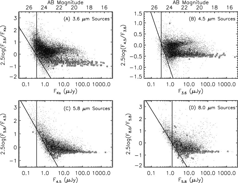
Figure 14.— $K_{S}$ and IRAC color-magnitude diagrams of IRAC selected sources. Dots show all sources selected at each corresponding IRAC band at $>3\sigma$. Gray squares show spectroscopically identified stars. In each panel, solid lines show the median $3\sigma$ detection limits of the two wavebands in consideration, adopted from Table 4.

7.1. Overlap with Other Catalogs

The GOODS-N has extremely rich multiwavelength data and several catalogs have been published of sources in this region. Here we summarize the overlap between these catalogs and our $K_{S}$ selected catalog.

In the GOODS-N and its flanking fields, the two most important optical observations are the HST ACS imaging of the GOODS-N (Giavalisco et al., 2004) and the Subaru SuprimeCam imaging of the $\sim 0.45$ deg field around the GOODS-N (Capak et al., 2004). In the 184 arcmin² HST ACS region, there are 16326 $K_{S}$ selected sources with S/N $>3$ in our catalog and 39432 $z^{\prime}$ (F850LP) selected ACS sources in the GOODS v2.0 catalog. With $0\farcs 4$ search radii ($0.5\times K_{S}$ seeing FWHM), 14291 (87.5%) $K_{S}$ sources have at least one ACS counterpart. The number increases to 14883 (91.2%) when the search radii are $0\farcs 8$. It increases much more slowly beyond this. Among the 1443 optically faint $K_{S}$ sources, 547 of them are detected at and 3.6 $\mu$m at $>3\sigma$. These are extremely unlikely spurious sources and appear to be truly optically faint NIR objects. The rest of the optically faint $K_{S}$ sources are either outside the IRAC region (407 sources) or do not have IRAC counterparts (489 sources). The later case may be an indication of the existence of spurious sources in our $K_{S}$ catalog (see § 5.2).

We can also reverse the direction of the counterpart search. Among the 39432 ACS sources, 16982 (43.1%) have at least one $K_{S}$ counterpart within $0\farcs 8$. The number decreases to 14853 (37.7%) for $0\farcs 4$ search radii. These show not only that the $K_{S}$ depth is insufficient for detecting most of the ACS sources, but also that the $K_{S}$ resolution is too low for separating some close pairs of galaxies in the ACS image.

Capak et al. (2004) released a Subaru SuprimeCam catalog of the GOODS-N region covering an area of 713 arcmin² with 48858 $R_{C}$+$z^{\prime}$ selected sources. In the same region, there are 51649 $K_{S}$ selected sources with S/N $>3$, among which 73.2% have counterparts in the Subaru catalog within $1\farcs 2$. The catalog of Capak et al. (2004) adopted a tighter S/N cut than our $K_{S}$ catalog. This partially explains why the fraction with optical counterparts here is much lower than in the ACS case, despite the fact that the Subaru images are very deep. The large scattering halos around bright stars in the Subaru image create “holes” in the catalog, and $K_{S}$ sources do not have optical counterparts in such holes.

The X-ray Chandra Deep Field-North (CDF-N) is fully covered by our $K_{S}$ imaging. The Chandra 2 Ms imaging (Alexander et al., 2003) covers an area of approximately 420 arcmin² with an uneven sensitivity distribution. There are 503 X-ray sources in the 2 Ms catalog, 493 (98.0%) of which have $K_{S}$ source counterparts within $2\farcs 5$ search radii. Among the 10 $K_{S}$-faint sources, four are close to the edge of relatively bright objects. The brighter $K_{S}$ objects may have affected the detection of the X-ray counterparts at $K_{S}$, or themselves may be the correct counterparts. To check whether the rest 6 are spurious X-ray sources, we look for their counterparts at other wavelengths. Two $K_{S}$-faint X-ray source (source #151 and #183 in the catalog of Alexander et al., 2003) have faint IRAC counterparts and are extremely faint in the optical. They are even close to two submillimeter sources detected at 1.1 mm (AzGN10 amd AzGN12 in Perera et al., 2008). Another (#88) has a faint optical counterpart but is outside the IRAC region. These three are therefore genuinely $K_{S}$-faint X-ray sources. Two $K_{S}$-faint X-ray sources (#248 and #371) are undetected in the Subaru optical, Spitzer 3.6 to 24 $\mu$m, and VLA 1.4 GHz images. Even in the X-ray images they appear to be quite faint. They are more likely spurious X-rayt sources. Finally, one X-ray source (#427) is not detected in any of the optical to radio images we have, but its detection appears quite convincing in the hard X-ray band. Its nature is undetermined.

The Spitzer GOODS Legacy Program also imaged the GOODS-N field with Multi-Band Imaging Photometer for Spitzer (MIPS, Rieke et al., 2004) at 24 $\mu$m. The GOODS Data Release 1+ provided a 24 $\mu$m catalog that is highly complete at 80 $\mu$Jy, containing 1199 sources. With search radii of $2\farcs 5$, 1182 MIPS sources have counterparts in our $K_{S}$ catalog. The rest are all in low S/N regions in the MIPS images and appear to be spurious. Thus, our $K_{S}$ image seems to detect all $>80$ $\mu$Jy 24 $\mu$m sources, bearing in mind the possibility that some sources could be misidentified by the large search radii.

Finally, at the long wavelength side, there exist deep VLA 1.4 GHz imaging in the GOODS-N (Richards, 2000). Biggs & Ivison (2006) re-reduced the VLA data and provided improved images and catalog. The catalog of Biggs & Ivison contains 537 $>30$ $\mu$Jy ($\sim 5\sigma$) 1.4 GHz sources within a radius of $\sim 24\arcmin$ centered at the HDF-N with a non-uniform sensitivity distribution. A total of 450 radio sources are within the $30\arcmin$ region of our $K_{S}$ image, 439 (97.5%) of which have $K_{S}$ counterparts within $1\farcs 5$ of search radii. The 11 $K_{S}$-faint radio sources do not appear to be spurious in the radio image, although some of them are very close to the $5\sigma$ limit at 1.4 GHz. They are all in the outer shallower region of the $K_{S}$ image. We note that, in the outer part of the image, the $K_{S}$ sensitivity decreases dramatically with exposure time (Figure 2), while the radio sensitivity decreases slowly with the primary beam of the VLA. We therefore conclude that the central part of our $K_{S}$ image is sufficiently deep for detecting nearly all of the 30 $\mu$Jy radio sources.

Figure 15.— $K_{S}$ and IRAC color-magnitude diagrams of X-ray, 24 $\mu$m, and 1.4 GHz selected sources. In panel (A) and (B), X-ray sources more luminous than $10^{42}$ erg s^-1 are enclosed by squares. Solid lines in each panel show median $3\sigma$ detection limits of the two wavebands in consideration.

7.2. Color-Magnitude Diagrams

In Figure 14 we present color-magnitude diagrams for sources selected in each of the four IRAC bands. The most apparent feature is the color bimodality in the $F_{3.6}/F_{Ks}$ and $F_{4.5}/F_{3.6}$ colors. There are two distinct, nearly horizontal branches. The blue branches contain most of the stars and low-redshift galaxies. The redshift divisions in $F_{3.6}/F_{Ks}$ and $F_{4.5}/F_{3.6}$ are $z\sim 0.7$ and $z\sim 1.2$, respectively. At these two redshifts, galaxies quickly move across the two branches, because of the rest-frame 1.6 $\mu$m SED bump in galaxies. This can also be seen in Figure 11, which is based on our spectroscopic redshifts. The division at $z\sim 1.2$ in the $F_{4.5}/F_{3.6}$ color is much more apparent in Figure 14 because Figure 11 suffers a bit from the spectroscopic redshift desert at $z\gtrsim 1.4$. The bimodality nearly disappears in the $F_{5.8}/F_{4.5}$ color and entirely disappears in the $F_{8.0}/F_{5.8}$ color. The main reason is that strong PAH emission from low-redshift starbursts significantly reddens the colors. A minor reason is the relatively lower S/N at these longer IRAC bands.

In Figure 15 we show the color-magnitude diagrams for the X-ray, 24 $\mu$m, and 1.4 GHz selected sources discussed in the previous subsections. The $F_{3.6}/F_{Ks}$ colors of all three populations lie in a well-defined area of the color-magnitude space. The distributions are determined by the sensitivities at X-ray, 24 $\mu$m and 1.4 GHz, plus loose correlations between luminosities at these wavebands (tracing star formation and black hole accretion) and the rest-frame 1–4 $\mu$m luminosities (tracing stellar mass). At bright magnitudes the sources are at low redshifts (the blue branch), while at the fainter fluxes the sources are at $z>0.7$ and the sources move to the red branch. The trend is the weakest for X-ray AGNs (open squares in Figure 15a), but it is still observable.

The distributions in the $F_{4.5}/F_{3.6}$ and $F_{5.8}/F_{4.5}$ colors of these three populations are more or less similar, and we do not show them here. However, the $F_{8.0}/F_{5.8}$ color-magnitude diagrams become significantly different. A group of red $F_{8.0}/F_{5.8}$ sources appear at the bright end. These colors are produced by strong PAH emission from low-redshift starbursting galaxies. They are also seen in the general 8 $\mu$m selected diagram (Figure 14d). It is interesting to note the difference between the low-luminosity X-ray sources (X-ray luminosity $<10^{42}$ erg s^-1, dots in Figure 15b) and the X-ray AGNs ($>10^{42}$ erg s^-1, squares in Figure 15b). In the Chandra 2 Ms sample, none of the X-ray AGNs have red $F_{8.0}/F_{5.8}$ colors of $>0.8$, because the strong radiation field of AGNs can destroy PAH molecules.

Figure 16.— $F_{4.5}/F_{3.6}$ vs. $F_{8.0}/F_{5.8}$ color-color diagrams of 8.0 $\mu$m ($>3\sigma$) and X-ray selected sources. In panel (B), X-ray AGNs ($>10^{42}$ erg s^-1) are enclosed with open squares. The dashed lines show the selection of $z>1.3$ galaxies proposed by B08, which is $\log(F_{4.5}/F_{3.6})>0.096\log(F_{8.0}/F_{5.8})$. The dotted lines show the selection of $z>1.2$ galaxies proposed by Devlin et al. (2009). The solid lines enclose the region where Stern et al. (2005) suggested that these colors select most broad-line AGNs.

7.3. IRAC Color-Color Diagrams

In B08 we presented $F_{4.5}/F_{3.6}$ vs. $F_{8.0}/F_{5.8}$ and $F_{5.8}/F_{3.6}$ vs. $F_{8.0}/F_{4.5}$ color-color diagrams along with our spectroscopic sample. With these two IRAC color-color diagrams, we analyzed efficiencies and contaminations of selections of $z>1.3$ and $z>1.6$ galaxies as well as AGNs. Since the quality of the IRAC photometry is improved here, it is interesting to revisit these issues. Here we focus on the selections of high-redshift galaxies and X-ray AGNs. (B08 also included the most powerful radio sources, but that sample size is very small.)

Figure 16 shows $F_{4.5}/F_{3.6}$ vs. $F_{8.0}/F_{5.8}$ color-color diagrams of 8.0 $\mu$m and X-ray selected sources. The color bimodality shown in Figure 14b is clearly seen here. The dashed lines are the $z>1.3$ selection proposed by B08. We reported in B08 that this selection can pick up 90% of $z>1.3$ galaxies, but 39% of the galaxies that satisfy this criterion are $z<1.3$ contaminants. In the 3$\sigma$ 8.0 $\mu$m sample here, there are 2096 spectroscopic redshifts, 352 of which are at $z>1.3$. The above selection picks up 241 of them, corresponding to a selection completeness of 68%, much lower than that in B08. On the other hand, the selection only picks up 54 $z<1.3$ galaxies, corresponding to a selection contamination of 18%, also much lower than that in B08. The results do not change much if we limit to higher S/N 8 $\mu$m sources where the measurements of colors are more robust. The inconsistency between the results here and our previous results is most likely a systematic difference in the calibration of the IRAC fluxes. For example, if we make the galaxies here $\sim 0.15$ magnitude redder in the $F_{4.5}/F_{3.6}$ color, then the completeness and contamination both become similar to those in B08.

The above comparison shows that using IRAC colors to select high-redshift galaxies is extremely sensitive to how galactic colors are measured. This also emphasizes that simply adopting existing IRAC color selection schemes may be problematic unless one is very careful about the fine details of the color measurements. Bearing this in mind, the selection completeness and contamination are then just a matter of fine tuning the selection criteria at the expense of one another. Such fine tuning also requires a relatively large sample of spectroscopic redshifts. In addition to the very likely difference in the colors, the basic conclusions about IRAC color selections on high-redshift galaxies remain unchanged here and in B08.

There are also other high-redshift galaxy selections. The dotted lines in Figure 16 show the $z>1.2$ selection adopted by Devlin et al. (2009) and Marsden et al. (2009) for studies of submillimeter galaxies. We found that all of the above conclusions apply to this selection as well. This selection has either incompleteness at high redshift or contaminations at low redshift.

Figure 17.— $F_{5.8}/F_{3.6}$ vs. $F_{8.0}/F_{4.5}$ color-color diagrams of 8.0 $\mu$m ($>3\sigma$) and X-ray selected sources. In panel (B), X-ray AGNs ($>10^{42}$ erg s^-1) are enclosed with open squares. The dashed lines show the selection of $z>1.6$ galaxies proposed by B08, which is $\log(F_{5.8}/F_{3.6})>0.096\log(F_{8.0}/F_{4.5})$. The solid lines enclose the region where Lacy et al. (2004) suggested that these colors select AGNs.

Figure 16b shows X-ray sources and X-ray AGNs. The IRAC colors suggested by Stern et al. (2005) to select most broad-line AGNs are enclosed by solid lines. However, here we see that the Stern et al. selection only picks up a fraction of the X-ray AGNs. By comparing both panels in Figure 16 as well as Figures 11b and d, we see that the same region also selects a larger number of high-redshift galaxies. These galaxies do not show up in the relatively shallow data of Stern et al. (2005, their Figure 1). This is consistent with the finding in B08 and Yun et al. (2008) that high-redshift reddened objects occupy similar color spaces to AGNs. The selection of Stern et al. (2005) does not pick up the majority of AGNs and has substantial galaxy contamination.

B08 also presented $F_{5.8}/F_{3.6}$ vs. $F_{8.0}/F_{4.5}$ color-color diagrams and used them to analyze selections of $z>1.6$ galaxies and the Lacy et al. (2004) selection of AGNs. As with the $F_{4.5}/F_{3.6}$ vs. $F_{8.0}/F_{5.8}$ color-color diagram, B08 concluded that the IRAC selection of $z>1.6$ galaxies can be very complete ($\sim 90\%$), but it has a large contamination ($\sim 40\%$) from low-redshift galaxies. B08 also found that the Lacy et al. (2004) selection of AGNs is incomplete (though better than the Stern et al., 2005 selection) and has severe galaxy contamination. We present the updated $F_{5.8}/F_{3.6}$ vs. $F_{8.0}/F_{4.5}$ color-color diagrams in Figure 17, and we confirm all the conclusions made by B08.

To sum up, using IRAC colors to select high-redshift galaxies can be either incomplete or suffer from contaminations from AGNs or low-redshift galaxies. The selection can be fine tuned to balance the completeness and contamination, but this requires a good spectroscopic sample and/or extremely well measured IRAC colors. We also found that galaxies and AGNs occupy a very similar region of color space. The IRAC selections of AGNs based on the Lacy et al. (2004) and Stern et al. (2005) methods always include large numbers of galaxy contaminations and have various degrees of incompleteness.

7.4. $K_{S}$ and IRAC Color-Color Diagrams

The above discussion only includes IRAC colors. In this work, we presented ultradeep $K_{S}$ photometry, which can be a powerful tool for studying galactic colors. We show the $F_{4.5}/F_{Ks}$ vs. $F_{4.5}/F_{3.6}$ color-color diagrams for 4.5 $\mu$m and X-ray sources in Figure 18. Here we only adopt the two shortest IRAC bands for their higher S/N and for their continuous availability in the Spitzer warm phase mission. Again, we see that the X-ray AGNs occupy a color space that is nearly identical to that of galaxies. Such a diagram is extremely ineffective for separating galaxies and AGNs. On the other hand, this color-color diagram is much more structured than the previous IRAC-only diagrams, suggesting that these colors can provide an excellent redshift diagnostic.

Figure 18.— $F_{4.5}/F_{Ks}$ vs. $F_{4.5}/F_{3.6}$ color-color diagrams of 4.5 $\mu$m ($F_{4.5}>2$ $\mu$Jy) and X-ray selected sources. In panel (B), X-ray AGNs ($>10^{42}$ erg s^-1) are enclosed with open squares.

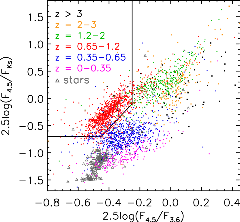
Figure 19.— $F_{4.5}/F_{Ks}$ vs. $F_{4.5}/F_{3.6}$ color-color diagram of spectroscopically identified sources in the B08 sample. Symbols are color coded with spectroscopic redshifts, including spectroscopically identified stars (gray triangles).

Figure 19 shows the same diagram as Figure 18, but only for the spectroscopic subsample drawn from B08. There is a very subtle difference in the distributions of galaxies in these two diagrams (4.5 $\mu$m selected vs. spectroscopically identified), because the spectroscopic identifications suffer from the redshift desert and are somewhat biased to galaxies with strong emission lines that can have unusual $F_{4.5}/F_{Ks}$ colors (see § 6.2.4). However, three distinct redshift groups can be seen in both diagrams: $z<0.65$, $z=0.65$–1.2, and $z>1.2$. In particular, we find that the following selection criteria are especially effective in selecting intermediate redshifts of $z=0.65$–1.2:

$$\log(F_{4.5}/F_{Ks})>-0.28\quad\quad{\rm and}$$

$$\log(F_{4.5}/F_{3.6})<-0.1\quad\quad{\rm and}$$

$$\log(F_{4.5}/F_{Ks})>1.2\log(F_{4.5}/F_{3.6})+0.26.$$

This selection is shown as the solid lines in Figure 19.

In Figure 19 a total of 2834 spectroscopic identifications are included, among which 1079 are at $z=0.65$–1.2. The above $K_{S}$ and IRAC selection picks up 870 galaxies at $z=0.65$–1.2, corresponding to a selection completeness of 81%. On the other hand, the selection also picks up 86 galaxies at $z<0.65$, 26 galaxies at $z>1.2$, and 3 stars, corresponding to a contamination of 11.6%. It is possible to fine tune the selection criteria to achieve higher completeness at the expense of increasing contamination, or vice versa. For example, after we moved the selecting region in the diagram towards the lower-right by 0.1 magnitude along both the $x$ and $y$ axes, the selection completeness increased to 89%, but the contamination also increased to 17%.

$F_{4.5}/F_{Ks}$ and $F_{4.5}/F_{3.6}$ colors can still be measured in the Spitzer warm phase mission and can be used in different ways. The above $z=0.65$–1.2 selection picks up galaxies at redshifts just lower than that in the popular $BzK$ selection ($z\sim 1.4$–2.5, Daddi et al., 2004). Galaxies at $z>1.2$ and $z<0.65$ can also be selected from the same diagram. In addition, in a subsequent paper, we will use the same diagram to select $z>2$ massive and dusty galaxies (Wang et al., in preparation).

Generally speaking, the addition of the $K_{S}$-band data increases the redshift resolution at $z<2$. At higher S/N this will greatly help IRAC-based photometric redshift studies (e.g., Pope et al., 2006), which can be more powerful than simple color selections. On the other hand, in all the examples discussed in this paper, IRAC colors become much less efficient in separating galaxies at $z>2$, even after the inclusion of $K_{S}$. For these high-redshift galaxies, optical colors or photometric redshifts that combine optical, NIR, and IRAC bands (e.g., Mancini et al., 2009) may be much better. However, on optically faint objects such as high-redshift submillimeter galaxies (e.g., Wang et al., 2007; Younger et al., 2009), colors from deep NIR and IRAC imaging are valuable in studying their redshifts.

8. Summary

We carried out ultradeep $K_{S}$ band imaging in the HDFN and its flanking field with WIRCam on the CFHT. The mosaic image has a size of $35\arcmin\times 35\arcmin$, fully covering the GOODS-N field. With nearly 50 hr of integration, we reached a 90% completeness limit of 1.38 $\mu$Jy ($\rm AB=23.55$) in the 0.25 deg² region, and 0.94 $\mu$Jy ($\rm AB=23.96$) in the 0.06 deg² GOODS-N IRAC region. The faintest detected objects have $K_{S}$ fluxes of $\sim 0.2$ $\mu$Jy ($\rm AB=25.65$). The photometry is uniform across the entire field, and the variation is well within 2%. In the GOODS-N region the astrometry is accurate to $0\farcs 03$ for compact objects with high S/N. The $K_{S}$ images and the associated catalogs are available through the internet.

We used the $K_{S}$ image and catalog as priors to measure MIR magnitudes in the Spitzer IRAC 3.6 to 8.0 $\mu$m bands with our REALCLEAN method. We verified the REALCLEAN results using data taken in two different epochs of observations, as well as by comparing our colors with the colors of stars and with the colors derived from model SEDs of galaxies at various redshifts. The REALCLEAN method appears to provide reasonably good photometry even on galaxies that have close neighbors within $2\arcsec$. This also provides a relatively clean way to identify faint IRAC objects that are not detected in the $K_{S}$ image. We make the REALCLEAN IRAC catalogs for both $K_{S}$ detected and undetected objects available to the community. Additional to the REALCLEAN method, we also measured galactic colors by convolving the $K_{S}$ image with the IRAC PSFs and convolving the IRAC images with the $K_{S}$ PSF. The derived colors are consistent with the REALCLEAN results.

We found our $K_{S}$ sample to be extremely powerful in studying the multiwavelength properties of high-redshift galaxies. The $K_{S}$ image detected most (if not all) of the X-ray, 24 $\mu$m, and radio sources published in this field. On the other hand, only 40% of the HST ACS sources in the GOODS-N are detected at $K_{S}$ at the current depth.

We studied various $K_{S}$ and IRAC color-magnitude and color-color diagrams. Because of the rest-frame 1.6 $\mu$m bump in the SEDs of galaxies, galaxies show significant color evolution in the $K_{S}$ and IRAC bands from $z=0$ to $z<2$. We found that using IRAC colors to select galaxies at certain redshifts is extremely sensitive to the color measurements and that balancing selection completeness and contamination will require careful tuning of the selection criteria with a good spectroscopic sample. We discussed an effective selection of $z=0.65$–1.2 galaxies using the $K_{S}$ band and the two shorter IRAC bands that will remain available in the Spitzer warm phase mission. We also confirmed our previous studies (B08) that the IRAC AGN selections in Lacy et al. (2004) and Stern et al. (2005) are either incomplete at the low-luminosity end or suffer severely from galaxy contamination.

References

- Alexander et al. (2003) Alexander, D. M. et al. 2003, AJ, 126, 539
- Anderson & King (2003) Anderson, J., & King, I. R. 2003, PASP, 115, 113
- Barger, Cowie, & Wang (2008) Barger, A. J., Cowie, L. L., & Wang, W.-H. 2008, ApJ, 689. 687 (B08)
- Bertin & Arnouts (1996) Bertin, E., & Arnouts, S. 1996, A&AS, 117, 393
- Biggs & Ivison (2006) Biggs, A. D. & Ivison, R. J. 2006, MNRAS, 371, 963
- Brinchmann & Ellis (2000) Brinchmann, J., & Ellis, R. 2000, ApJ, 536, L77
- Calzetti et al. (2000) Calzetti, D., Armus, L., Bohlin, R. C., Kinney, A. L., Koornneef, J., & Storchi-Bergmann, T. 2000, ApJ, 533, 682
- Capak et al. (2004) Capak, P., et al. 2004, AJ, 127, 180
- Capak et al. (2007) Capak, P., et al. 2007, ApJS, 172, 99
- Cohen, Wheaton, & Megeath (2003) Cohen, M., Wheaton, Wm. A., & Megeath, S. T. 2003, AJ, 126, 1090
- Cornwell, Braun, & Briggs (1999) Cornwell, T., Braun, R., & Briggs, D. S. 1999, in ASP Conf. Ser. 180, Synthesis Imaging in Radio Astronomy II, e.d. G. B. Taylor, C. L. Carilli, & R. A. Perley, 151
- Cowie et al. (1994) Cowie, L. L., Gardner, J. P., Hu, E. M., Songaila, A., Hodapp, K.-W., & Wainscoat, R. J. 1994, ApJ, 434, 114
- Cowie & Barger (2008) Cowie, L. L., & Barger, A. J. 2008, ApJ, 686, 72
- Cutri et al. (2003) Cutri, R. M., et al. 2003, Explanatory Supplement to the 2MASS All Sky Data Release (Washington: NASA), http://www.ipac.caltech.edu/2mass/releases/allsky/doc/explsup.html
- Daddi et al. (2004) Daddi, E., Cimatti, A., Renzini, A., Fontana, A., Mignoli, M., Pozzetti, L., Tozzi, P., & Zamorani, G. 2004, ApJ, 617, 746
- Devlin et al. (2009) Devlin, M. J., et al. 2009, Nature, 458, 737
- Elsner et al. (2008) Elsner, F., Feulner, G., & Hopp, U. 2008, A&A, 477, 503
- Fazio et al. (2004) Fazio, G. G., et al. 2004, ApJS, 154, 10
- Fontana et al. (2006) Fontana, A., et al. 2006, A&A, 459, 745
- Giavalisco et al. (2004) Giavalisco, M. et al. 2004, ApJ, 600, L93
- Grazian et al. (2006) Grazian, A., et al. 2006a, A&A, 449, 951
- Hatziminaoglou et al. (2005) Hatziminaoglou, E., et al. 2005, AJ, 129, 1198
- Högbom (1974) Högbom, J. A. 1974, A&AS, 15, 417
- Kajisawa et al. (2006) Kajisawa, M., et al. 2006, PASJ, 58, 951
- Kajisawa et al. (2009) Kajisawa, M., et al. 2009, ApJ, 702, 1393
- Kauffmann & Charlot (1998) Kauffmann, G., & Charlot, S. 1998, MNRAS, 297, L23
- Keenan et al. (2010) Keenan, R. C., Trouille, L., Barger, A. J., Cowie, L. L., & Wang, W.-H. 2010, ApJS, 186, 94
- Kinney et al. (1996) Kinney, A. L., Calzetti, D., Bohlin, R. C., McQuade, K., Storchi-Bergmann, T., & Schmitt, H. R. 1996, ApJ, 467, 38
- Lacy et al. (2004) Lacy, M., et al. 2004, ApJS, 154, 166
- Laidler et al. (2007) Laidler, V. G., et al. 2007, PASP, 119, 1325
- Mancini et al. (2009) Mancini, C., Matute, I., Cimatti, A., Daddi, E., Dickinson, M., Rodighiero, G., Bolzonella, M., & Pozzetti, L. 2009, A&A, 500, 705
- Marsden et al. (2009) Marsden, G., et al. 2009, ApJ, in press (arXiv:0904.1205)
- Perera et al. (2008) Perera, T. A., et al. 2008, MNRAS, 391, 1227
- Pérez-González et al. (2008) Pérez-González, P. G., et al. 2008, ApJ, 686, 72
- Pope et al. (2006) Pope, A., et al. 2006, MNRAS, 370, 1185
- Richards (2000) Richards, E. A. 2000, ApJ, 533, 611
- Reddy et al. (2006) Reddy, N. A., Steidel, C. C., Erb, D. K., Shapley, A. E., & Pettini, M. 2006, ApJ, 653, 1004
- Reach et al. (2005) Reach, W. T., et al. 2005, PASP, 117, 978
- Rieke et al. (2004) Rieke, G., et al. 2004, ApJS, 154, 25
- Sajina, Lacy, & Scott (2005) Sajina, A., Lacy, M., & Scott, D. 2005, ApJ, 621, 256
- Sawicki (2002) Sawicki, M. 2002, AJ, 124, 3050
- Silva et al. (1998) Silva, L., Granato, G. L., Bressan, A., & Danese, L. 1998, ApJ, 509, 103
- Simpson & Eisenhardt (1999) Simpson, C., & Eisenhardt, P. 1999, PASP, 111, 691
- Skrutskie et al. (2006) Skrutskiee, M. F., et al. 2006, AJ, 131, 1163
- Stern et al. (2005) Stern, D., et al. 2005, ApJ, 631, 163
- Wang et al. (2007) Wang, W.-H., Cowie, L. L., van Sader, J., Barger, A. J., & Williams, J. P. 2007, ApJ, 670, L89
- Wang, Barger, & Cowie (2009) Wang, W.-H., Barger, A. J., & Cowie, L. L., 2009, ApJ, 690, 319
- Younger et al. (2009) Younger, J. D., et al. 2009, ApJ, 704, 803
- Yun et al. (2008) Yun, M. S., et al. 2008, MNRAS, 389, 333