Bringing entanglement to the high temperature limit

Abstract

We show the existence of an entangled nonequilibrium state at very high temperatures when two linearly coupled harmonic oscillators are parametrically driven and dissipate into two independent heat baths. This result has a twofold meaning: first, it fundamentally shifts the classical-quantum border to temperatures as high as our experimental ability allows us, and second, it can help increase by at least one order of magnitude the temperature at which current experimental setups are operated.

Introduction.— Since the establishment of quantum theory in last century there has been a long evolution on our concept of what is quantum and to what extent it is required to explain observations in nature. At the very beginning the reduction postulate was proposed, clearly separating between quantum microscopic entities and classical macroscopic measuring apparatuses. Since then macroscopic quantum phenomena such as superconductivity and coherent superposition in Bose–Einstein condensates Andrews et al. (1997), together with interference fringes of very massive molecules Hornberger et al. (2009) have been observed. Recently a proposal to create superpositions of dielectric bodies, such as viruses up to micron size, inside a high finesse optical cavity has been given Romero-Isart et al. (2009). Hence the border between the classical and quantum worlds seems to be more diffuse and intriguing than we could have conceived one century ago.

Neither the usual transition criterion of $\hbar/S_{ch}\rightarrow 0$ (with $S_{ch}$ the characteristic action of the system) is to be trusted, since this limit could be not completely continuous and strong deviations have been reported in the semiclassical regime Dittrich and Pachón (2009). In the more realistic situation when the system interacts with the surrounding environment, dissipation restricts purely quantum phenomena to within the very low temperatures limit Zurek (2003),

$$k_{B}T/\hbar\omega\ll 1\;,$$ (1)

where $\hbar\omega$ denotes the typical energy scale of the system and $k_{B}T$ the thermal energy. Above this limit, quantum correlations are inaccessible behind a ’mask’ of thermal fluctuations.

As a consequence, observing quantum phenomena implies the need for a very delicate pre-cooling process. But, is there any alternative to cooling for being quantum? In the present Letter, we defy the above classicality criterion and report the existence of a nonequilibrium entangled steady state for coupled harmonic oscillators at high temperatures, obtained through parametric driving. This result is quite fundamental, meaning that we might expect entanglement in hot highly nonequilibrium situations, as pointed out Cai et al. (2008) for biological systems. Further, it could lighten the burden on quantum experiments requiring delicate pre-cooling setups. We note that though quantum coherence can play a role in biological processes at ambient temperature Collini et al. (2010), demonstration of entanglement would be a much more extreme phenomenon.

The model and its solution.— In order to render our arguments more quantitative, we study the entanglement between two interacting identical harmonic oscillators. Though an idealization, it encompasses a reasonable description of a wide variety of objects in nature such as nanomechanical oscillators Schwab and Roukes (2005), optical Gröblacher et al. (2009) and microwave cavities Wallraff et al. (2004), and movable mirrors Marshall et al. (2003) to cite some, through which we expect to give a character of universality to the concepts that we expose here. The Hamiltonian of the system, $\mathcal{H}_{\rm s}$ reads

$$\mathcal{H}_{\rm s}=\sum_{\alpha=1}^{2}\left(\frac{P_{\alpha}^{2}}{2m}+\frac{1}{2}m\omega^{2}Q_{\alpha}^{2}\right)+c(t)\;Q_{1}Q_{2}\;,$$ (2)

with $m$ the mass of the oscillator, $\omega$ the frequency and $c(t)$ is the coupling coefficient. In what follows we assume:

$$\frac{c(t)}{m}=c_{0}+c_{1}\cos(\omega_{\rm d}t)\;,$$ (3)

that is, we consider a time dependent interaction, which plays a fundamental role in the creation and survival of entanglement.

In any realistic scenario the system is not completely isolated from the outside. The most rigorous way to include dissipation is by means of the system-bath model Weiss (1993). We couple the oscillators to two independent baths (see figure 1a),

$${\cal H} = \mathcal{H}_{\rm s}+\sum_{\alpha,k=1}^{2,\infty}\frac{{p_{\alpha,k}}^{2}}{2{m}_{k}}+\frac{{m}_{k}{\omega}_{k}^{2}}{2}\left({x_{\alpha,k}}-\frac{{c}_{k}Q_{\alpha}}{{m}_{k}{\omega}_{k}^{2}}\right)^{2}\;,\;\;$$ (4)

where the baths are modeled by an infinite collection of harmonic oscillators Ullersma (1966); Caldeira and Leggett (1983). This independence accounts for a bath having a characteristic correlation length which exceeds the distance between oscillators. The opposite case corresponds to a model with common bath Paz and Roncaglia (2008) and leads to conservation of quantum entanglement at higher than $\hbar\omega/k_{B}$ temperatures. This can be shown to be spurious since having different oscillator frequencies or bath couplings (and no driving) leads again to the diagram in figure 1b. Therefore we place ourselves in the most pessimistic situation for studying entanglement Liu and Goan (2007).

The evolution for the density matrix of the two oscillators, ${\hat{\rho}}_{s}$, can be cast as,

$$\rho_{s}(X_{f},t)=\int{\rm d}^{4}X_{i}J(X_{f},t;X_{i},0)\rho_{s}(X_{i},0),$$ (5)

with $X=\{Q_{1,+},Q_{1,-},Q_{2,+},Q_{2,-}\}$ and $J(X_{f},t;X_{i},0)$ being the influence functional which is given in terms of a path integral expression after tracing out the environmental degrees of freedom Feynman and Vernon F. L. (1963). Usually, the analytical evaluation of $J(X_{f},t;X_{i},0)$, even for time independent systems, is only possible in very few cases Caldeira and Leggett (1983); Grabert et al. (1988). Here, we have been able to derive an exact analytic expression for $J(X_{f},t;X_{i},0)$ in terms of the odd and even solutions of the Mathieu oscillator (See Appendices B and C). The environmental influence enters via the spectral density $I(\omega)=\sum_{j}c_{j}^{2}/(2m_{j}\omega_{j})\delta(\omega-\omega_{j})$. Here, we assume for simplicity Ohmic noise $I(\omega)=m\gamma\omega$. It produces white noise in the classical limit Grabert et al. (1988). With our analytical result we can study the central system in any regime: low or high temperature, strong or weak damping, deeply quantum or semiclassical energy scales, etc., thus avoiding any spurious approximative corrections or limitations. As a result, any system that can be considered as two harmonic oscillators with linear coupling can be ascribed exactly to our description.

Entanglement computation.— Linearity of the total Hamiltonian ensures that the state is always Gaussian, and thus its entanglement properties are fully characterized by the covariance matrix $\sigma_{i,j}=\langle\xi_{i}\xi_{j}+\xi_{j}\xi_{i}\rangle/2-\langle\xi_{i}\rangle\langle\xi_{j}\rangle$ with $\xi=(Q_{1},Q_{2},P_{1},P_{2})$. An exact measure of entanglement is known for Gaussian states, the Logarithmic Negativity $E_{N}$, as explained in Appendix A. It is computed from the covariance matrix, which can be calculated from the propagator $J(X_{f},t;X_{i},0)$ (see appendix E). In what follows we will exclusively use this measure.

Entanglement in the time independent case.— In contact with an environment, each particle is asymptotically forced into a thermal state with a temperature equal to that of the bath it is connected to. This state is reached independently on the initial condition of the oscillator, which in the case of no driving [$c_{1}=0$ in (3)] leads to the entanglement characteristics shown in figure (1b). That is, any state will, after thermalization, fall into either the blue (entangled) part or the white (separable) part, depending only on the ratio $c_{0}/m\omega^{2}$ and the bath’s temperatureLiu and Goan (2007) . The entanglement region is restricted to the so called quantum limit $\hbar\omega<kT$, as expected from intuition, above such a temperature each oscillator has an independent description because the quantum state is separable .

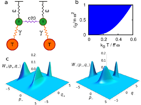
Figure 1: Generation of an entangled nonequilibrium state with dissipative environments. a, The system is formed by two linearly coupled oscillators, initially thermalised due to each of them being dissipatively coupled to an environment at temperature $T$. Driving sinusoidally the coupling leads to production of entanglement even at very high temperatures. b, Entanglement phase diagram for the case without driving. The state thermalizes to a state with no entanglement unless the temperature is below the quantum limit $k_{\rm B}T<\hbar\omega$. c, Wigner phase-space representation of the normal modes. They are squeezed along orthogonal directions, so the oscillators are entangled ($E_{N}\simeq 0.33$). The parameters are $k_{B}T/\hbar\omega=10$, $\gamma=0.01\omega$, $c_{1}=0.5m\omega^{2}$, while the snapshot has been taken at time $\omega t=6$.

Entanglement creation by driving— We sketch here a simple idea of how to produce an entangled nonequilibrium state at high temperatures. It may provide a huge leap in experimental requirements , while in addition it definitely removes temperature from the list of possible criteria for classicality, the latter being an important theoretical topic. The normal mode transformation for the oscillator Hamiltonian (2) reads $\widetilde{H}=\sum_{\alpha=\pm}P_{\alpha}^{2}/2m+\omega_{\pm}^{2}Q_{\alpha}/2$ where $Q_{\pm}=(Q_{1}\pm Q_{2})/\sqrt{2}$ ($P_{\pm}=(P_{1}\pm P_{2})/\sqrt{2}$) and $\omega_{\pm}^{2}=\omega\pm c(t)/m$. In the continuous variable setting, it is known that the maximally entangled state -a kind of reference state, comparison with which provides a quantification scheme for entanglement- is the Einstein, Podolsky, Rosen wavefunction Einstein et al. (1935). It is just the infinite squeezing limit of the two-mode squeezed vacuum state, in which the indeterminacies of $Q_{+}$ and $P_{-}$ are under the standard quantum limit set by Heisenberg’s principle, while $Q_{-}$ and $P_{+}$ are above it (such that $\Delta Q_{\pm}/\Delta P_{\pm}=\exp{(\mp 2r)}/\omega^{2}$, with $r$ the so-called squeezing parameter). The opposite situation is also valid. Thus generation of entanglement can be provided by squeezing of the normal modes, which in turn can be generated through parametric driving of their frequencies Galve and Lutz (2009). Both a time dependence in $\omega$ or $c$ will do, however the latter is better because it naturally provides the correct combination of squeezing between $\pm$ modes. At the same time, the environment will try to destroy quantum coherence through equilibration to the thermal state. Thus we have two competing effects, whose balance will determine whether the steady state is entangled or not. In figure 1 we provide an example of normal mode squeezing in presence of the bath above the typical quantum limit (1) $k_{B}T/\hbar\omega=10>1$.

In figure 2 we summarize our results. Indeed, we find sets of parameters where entanglement is present at temperatures beyond the quantum limit, notice that in both figures $k_{\rm B}T>\hbar\omega$. Starting with a thermal state at the bath’s temperature, the system reaches after a certain time a nonequilibrium steady state with nonzero entanglement. We have chosen rather conservative couplings to the baths, as we will explain later, and still very high temperatures, $k_{\rm B}T\gg\hbar\omega$, can be reached.

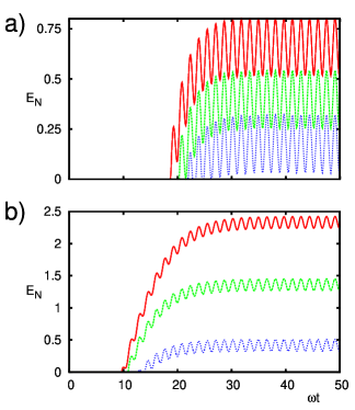
Figure 2: (Color online) a, Time evolution of entanglement under parametric driving of the coupling at different environmental temperatures $k_{B}T/\hbar\omega=250$(red), $300$(green), $350$(blue), with a damping of $\gamma=0.005\omega_{0}$, driving amplitude of $c_{1}=0.5m\omega_{0}^{2}$ and driving frequency $\omega_{d}=2\times 0.998\omega_{0}$. A steady entangled state is reached in a reasonable time with a significative amount of entanglement. b, Now the temperature is kept fix , $k_{B}T/\hbar\omega=5$, with the same parameters, while the damping parameter is varied: $\gamma=0.005\omega_{0}$(red), $0.01\omega_{0}$(green), $0.02\omega_{0}$(blue).

It is a remarkable fact that while the system is forced into a highly nonequilibrium state, a steady state of entanglement is reached which is independent on the initial state of the system. To show this effect we plot in figure 3 (see inset) the time evolution of entanglement when the system starts with a two mode squeezed state and squeezing parameters $r=0,0.5,1$, and compare it to the case of an initial thermal state with the same temperature as the bath.

New ’phase diagram’ for entanglement— Parametric driving yields a new asymptotic behaviour which defines a new ’phase diagram’, now dependent on four parameters: driving amplitude and frequency, temperature and the coupling to the bath. The driving frequency is overall chosen to be $\omega_{d}=2\times 0.998\omega$, and we also set $c_{0}=0$. While the optimal squeezing generation is obtained with a $\omega_{d}$ dependent on $\omega$ and $c_{1}$, the latter number seems to produce results nearly as good for different parameters, so it will be used unless otherwise stated. In figure 3 we see the points which delimit the border between presence(left)/absence(right) of entanglement, which is linear in temperature and driving amplitude and, as expected, the more isolated and driven the system is (low $\gamma$ and high $c_{1}$), the higher the temperature can be reached. In addition to the exact result, we have plotted a simple estimation of the border which we explain next.

We already mentioned that the entanglement production in this system can be viewed as a competition between the squeezing due to the driving and mixing because of the environment. The rate of squeezing can be obtained from the solutions to the nondissipative driven problem. They have the Mathieu form $x(t)=\exp{(i\mu_{M}t)}\phi(t)$, where $\phi(t)$ is a periodic function.If the Mathieu characteristic exponent $\mu_{M}$ is real, they are stable, otherwise they are divergent which implies production of squeezing at a rate $|$Im$(\mu_{M})|$ (for every damped solution there is a divergent one) Zerbe and Hänggi (1995). The rate of decoherence can be estimated from the diffusion coefficient $D$Zurek (2003) (see Appendix D), yielding $\gamma D\sim\gamma\ k_{B}T/\hbar\omega$ whenever $k_{B}T>\hbar\omega$. Thus by comparison of both rates we obtain the new condition under which entanglement is present:

$$\frac{k_{B}T}{\hbar\omega}\leq\frac{|\rm{Im}(\mu_{M})|}{\gamma}\;,$$ (6)

which is seen to be a rather impressive match to the exact evolution. The condition above should be compared with the standard condition (1). In a nutshell the driving brings in a new quantum limit.

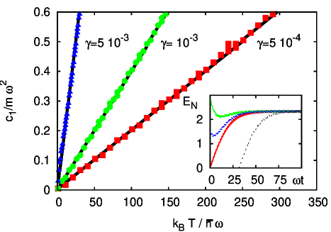
Figure 3: ’Phase diagram’ of entanglement in the presence of parametric driving. We compare the condition (6) [lines] with the exact time evolution [dots] for different bath couplings $\gamma=0.005\omega$ (blue triangles), $0.001\omega$ (green circles ) and $0.0005\omega$ (red squares). Inset: time evolution for different initial conditions, namely a two mode squeezed vaccuum state (dotted curves) with squeezing parameter $r=0$ (red), $0.5$ (blue), $1$ (green), as compared to that of an initial thermal state (black). They all converge after some tens of periods. The parameters here are $\gamma=0.001\omega$, $c_{1}=0.2m\omega^{2}$, $\omega_{d}=2\times 0.9998\omega$ and $k_{B}T/\hbar\omega=10$.

Some examples— We give next some actual examples of experiments which could profit from our strategy. However an additional comment is in order: the fact that squeezing grows approximately as $|\text{Im}(\mu_{M})|t$ also means that the energy and delocalization in space are increasing exponentially in time. Thus checking consistency with experimental size and energy considerations is a must.

Take for example two Calcium ions, each confined in its own planar Penning traps Stahl et al. (2005). A trap can be fabricated by nanolithography with a size of $d\sim 0.12\mu m$. If a voltage of $V=10V$ is applied, the motional frequency is $\omega\simeq 21$GHz and thus we can interpret figure 1 as the temperature in Kelvin. A wire mediated capacitive coupling between traps allows to reduce the effective distance between ions and makes the coupling increase up to a reasonable level $c(t)=c_{0}=0.047m\omega_{0}^{2}$. If the frequencies are driven instead of the coupling (i.e. $\omega(t)=\omega_{0}+\omega_{1}\sin\omega_{d}t$), and assuming $\gamma=0.0005\omega$, we still manage to get entanglement up to $\sim 50K$, while the delocalization of the oscillators is yet below the trap size, ensuring no confinement leakage. To reach room temperature a very strong coupling would be required indeed, but our method allows the experimentalist to avoid building a sub-4K (liquid Helium) setup. We believe this to be a huge experimental step.

Another example is microwave superconducting cavities Mariantoni et al. (2008). The coupling between two cavities can be modulated placing a superconducting qubit between them. The effective hamiltonian governing the dynamics is (2). The typical frequencies in these resonators are in the GigaHerz regime, operating usually in the milikelvin range. The decoherence in these systems is $\gamma\cong 10^{-4}\omega$, or even less. However the coupling is weak, around $10$MHz. In this case, due to the weak coupling, the parametric driving would enhance the amount entanglement that could be measured by nowadays technology Menzel et al. (2010).

Current experiments with nanomechanical resonators have these typical parameters: $\omega=2\pi\nu=2\pi\times 15{\rm MHz}$, $m=10^{-17}{\rm kg}$, $c_{1}\sim 10^{-1}m\omega^{2}$, and a quality factor $Q\sim 20000$, which yields a damping $\gamma=5\times 10^{-5}\omega$ Woolley et al. (2008). An entangled state can be observed at $2K$. If the frequency can be increased a factor 10, it might reach the entangled regime in presence of liquid Helium.

In addition it is notable that the strong coupling regime has been reached between a massive mechanical microresonator and light Gröblacher et al. (2009). Furthermore, a proposal for parametrically driving the coupling between a nanomechanical resonator and a superconducting electrical resonator has been given in Tian et al. (2008). Thus we might well foresee that these advances could be used to measure entanglement in yet unsuspected temperature regimes in the near future, while eliminating the need for complex and costly setups to cool objects to the quantum regime.

Acknowledgments— We aknowledge Peter Hänggi and Gert-Ludwig Ingold for enlightened discussions and advices. We also thank the warm hospitality from the Universität Augsburg where this work was started. DZ aknowledges financial suport from FIS2008-01240 (MICINN), FG from COQUSYS (IFISC-CSIC), LAP from Colciencias and the U. Nal. de Colombia.

Appendix A Entanglement quantification

Entanglement can be easily quantified for a bipartite system of continuous variables in a Gaussian state. The logarithmic negativity Vidal and Werner (2002) gives a characterization of the amount of entanglement which can be distilled into singlets. In the case of Gaussian continuous variable states, only the covariance matrix is needed. The covariance matrix $\sigma$ is defined as

$$\sigma_{\xi_{i}\xi_{j}}=\langle\xi_{i}\xi_{j}+\xi_{j}\xi_{i}\rangle/2-\langle\xi_{i}\rangle\langle\xi_{j}\rangle$$ (7)

with $\xi_{i}=Q_{1},Q_{2},P_{1},P_{2}$. The logarithmic negativity is defined as

$$E_{N}=-\frac{1}{2}\sum_{i=1}^{4}\log_{2}[\text{Min}(1,2|l_{i}|)]$$ (8)

where $l_{i}$ are the symplectic eigenvalues of the covariance matrix. They are simply the normal eigenvalues of the matrix $-i\Sigma\sigma$, with $\Sigma$ the symplectic matrix

$$\sigma=\left(\begin{array}[]{cc}0&\textbf{1}_{2}\\ -\textbf{1}_{2}&0\end{array}\right)$$ (9)

and $\textbf{1}_{2}$ is the $2\times 2$ identity matrix.

Whenever the logarithmic negativity of the system is zero, we have a separable state $\rho_{s}=\sum_{i}p_{i}\rho_{1}^{(i)}\otimes\rho_{2}^{(i)}$, and each oscillator can be described independently. In continuous variable systems, the amount of entanglement is unbounded from above, having as a limiting case the maximally entangled EPR wavefunction with $E_{N}\to\infty$.

Appendix B Decoupling the total system in normal modes

The Hamiltonian of the total system reads

$$\mathcal{H}_{\rm s} = \frac{p_{1}^{2}}{2m}+\frac{1}{2}m\omega^{2}q_{1}^{2}+\frac{p_{2}^{2}}{2m}+\frac{1}{2}m\omega^{2}q_{2}^{2}+c(t)q_{1}q_{2},$$ (10)

$${H}_{IB} = \sum_{k=1}^{N}\frac{1}{2m_{k}}p_{k}^{2}+\frac{1}{2}m_{k}\omega_{k}^{2}\left(x_{k}-\frac{c_{k}q_{1}}{m_{k}\omega_{k}^{2}}\right)^{2}+\sum_{k=1}^{N}\frac{1}{2{m^{\prime}}_{k}}{p^{\prime}}_{k}^{2}+\frac{1}{2}{m^{\prime}}_{k}{\omega^{\prime}}_{k}^{2}\left({x^{\prime}}_{k}-\frac{{c^{\prime}}_{k}q_{2}}{{m^{\prime}}_{k}{\omega^{\prime}}_{k}^{2}}\right)^{2},$$ (11)

where $c(t)=mc_{0}+mc_{1}\cos(\omega_{\rm d}t)$. Introducing the normal modes coordinates $x_{+}$ and $x_{-}$ defined by

$$q_{1}=\frac{1}{\sqrt{2}}\left(x_{+}+x_{-}\right),\qquad p_{1}=\frac{1}{\sqrt{2}}\left(p_{+}+p_{-}\right),$$ (12)

$$q_{2}=\frac{1}{\sqrt{2}}\left(x_{+}-x_{-}\right),\qquad p_{2}=\frac{1}{\sqrt{2}}\left(p_{+}-p_{-}\right),$$ (13)

$\mathcal{H}_{\rm s}$ reads

$${\cal H}_{S} = \frac{p_{+}^{2}}{2m}+\frac{1}{2}m\Omega_{+}^{2}(t)x_{+}^{2}+\frac{p_{-}^{2}}{2m}+\frac{1}{2}m\Omega_{-}^{2}(t)x_{-}^{2},$$ (14)

where $\Omega_{\pm}^{2}(t)=\omega^{2}\pm c(t)/m$ and $H_{IB}$

$${H}_{IB} = \sum_{k=1}^{N}\frac{1}{2m_{k}}p_{k}^{2}+\frac{1}{2}m_{k}\omega_{k}^{2}x_{k}^{2}-\frac{1}{\sqrt{2}}c_{k}x_{k}(x_{+}+x_{-})+\frac{c_{k}^{2}}{2\sqrt{2}m_{k}\omega_{k}^{2}}(x_{+}+x_{-})^{2}$$ (15)

$$+ \sum_{k=1}^{N}\frac{1}{2{m^{\prime}}_{k}}{p^{\prime}}_{k}^{2}+\frac{1}{2}{m^{\prime}}_{k}{\omega^{\prime}}_{k}^{2}{x^{\prime}}_{k}^{2}-\frac{1}{\sqrt{2}}{c^{\prime}}_{k}{x^{\prime}}_{k}(x_{+}-x_{-})+\frac{{c^{\prime}}_{k}^{2}}{2\sqrt{2}{m^{\prime}}_{k}{\omega^{\prime}}_{k}^{2}}(x_{+}-x_{-})^{2}.$$

These coordinates introduce a cross-term $x_{+}x_{-}$, which cancels out if

$$\frac{c_{k}^{2}}{m_{k}\omega_{k}^{2}}=\frac{{c^{\prime}}_{k}^{2}}{{m^{\prime}}_{k}{\omega^{\prime}}_{k}^{2}}.$$ (16)

This requirement does not means that the oscillators in the baths are identic but their modes distributions. In the continuous limit, it implies that the spectral distributions characterizing the baths, $J_{1}(\omega)$ and $J_{2}(\omega)$, are the same. In this case,

$${H}_{IB} = \sum_{k=1}^{N}\left\{\frac{1}{2m_{k}}p_{k}^{2}+\frac{1}{2}m_{k}\omega_{k}^{2}x_{k}^{2}+\frac{1}{2{m^{\prime}}_{k}}{p^{\prime}}_{k}^{2}+\frac{1}{2}{m^{\prime}}_{k}{\omega^{\prime}}_{k}^{2}{x^{\prime}}_{k}^{2}+\frac{c_{k}^{2}}{\sqrt{2}m_{k}\omega_{k}^{2}}x_{+}^{2}+\frac{c_{k}^{2}}{\sqrt{2}m_{k}\omega_{k}^{2}}x_{-}^{2}\right.$$ (17)

$$- \left.\left(\frac{1}{\sqrt{2}}{c}_{k}{x}_{k}+\frac{1}{\sqrt{2}}{c^{\prime}}_{k}{x^{\prime}}_{k}\right)x_{+}-\left(\frac{1}{\sqrt{2}}{c}_{k}{x}_{k}-\frac{1}{\sqrt{2}}{c^{\prime}}_{k}{x^{\prime}}_{k}\right)x_{-}\right\}.$$

This expression suggests the introduction of new set of coordinates $\mathfrak{q}_{k}$ and $\mathfrak{Q}_{k}$ defined by

$$\mathfrak{q}_{k}=\frac{1}{\lambda_{k}\sqrt{2}}\left({c}_{k}{x}_{k}+{c^{\prime}}_{k}{x^{\prime}}_{k}\right), \mathfrak{Q}_{k}=\frac{1}{\Lambda_{k}\sqrt{2}}\left({c}_{k}{x}_{k}-{c^{\prime}}_{k}{x^{\prime}}_{k}\right),$$ (18)

which can be inverted

$$x_{k}=\frac{1}{\sqrt{2}{c}_{k}}\left(\lambda_{k}{\mathfrak{q}}_{k}+\Lambda_{k}{\mathfrak{Q}}_{k}\right), {x^{\prime}}_{k}=\frac{1}{\sqrt{2}{c^{\prime}}_{k}}\left(\lambda_{k}{\mathfrak{q}}_{k}-\Lambda_{k}{\mathfrak{Q}}_{k}\right),$$ (19)

$$p_{k}=\frac{1}{\sqrt{2}{c}_{k}}\left(\lambda_{k}{\mathfrak{p}}_{k}+\Lambda_{k}{\mathfrak{P}}_{k}\right), {p^{\prime}}_{k}=\frac{1}{\sqrt{2}{c^{\prime}}_{k}}\left(\lambda_{k}{\mathfrak{p}}_{k}-\Lambda_{k}{\mathfrak{P}}_{k}\right).$$ (20)

After substituting in $H_{IB}$ and choosing $m_{k}c_{k}^{2}={m^{\prime}}_{k}{c^{\prime}}_{k}^{2}$ to eliminate a term proportional to $\mathfrak{p}_{k}\mathfrak{P}_{k}$, we have

$${H}_{IB} = \sum_{k=1}^{N}\left\{\frac{\lambda_{k}^{2}}{2m_{k}c_{k}^{2}}\mathfrak{p}_{k}^{2}+\frac{m_{k}\omega_{k}^{2}\lambda_{k}^{2}}{2c_{k}^{2}}\mathfrak{q}_{k}^{2}-\lambda_{k}\mathfrak{q}_{k}x_{+}+\frac{\Lambda_{k}^{2}}{2m_{k}c_{k}^{2}}\mathfrak{P}_{k}^{2}+\frac{m_{k}{\omega}_{k}^{2}\Lambda_{k}^{2}}{2c_{k}^{2}}{\mathfrak{Q}}_{k}^{2}-\Lambda_{k}\mathfrak{Q}_{k}x_{-}\right\}.$$ (21)

To obtain a more standard version of the Hamiltonian, we could redefine $m_{k}\rightarrow\lambda_{k}^{2}/c_{k}^{2}\mathfrak{m}_{k}$ and $\omega_{k}^{2}=c_{k}^{2}\varpi_{k}^{2}/\lambda_{k}^{4}$ and impose $\lambda_{k}^{2}=\Lambda_{k}^{2}$ or just by choosing $\lambda_{k}^{2}=c_{k}^{2}=\Lambda_{k}^{2}$, so

$${H}_{IB} = \sum_{k=1}^{N}\left\{\frac{1}{2m_{k}}\mathfrak{p}_{k}^{2}+\frac{m_{k}\omega_{k}^{2}}{2}\mathfrak{q}_{k}^{2}\pm c_{k}\mathfrak{q}_{k}x_{+}+\frac{1}{2m_{k}}\mathfrak{P}_{k}^{2}+\frac{m_{k}{\omega}_{k}^{2}}{2}{\mathfrak{Q}}_{k}^{2}\pm c_{k}\mathfrak{Q}_{k}x_{-}\right\}.$$ (22)

It means that we can conserve a small arbitrariness in the phase of the coupling by choosing different signs by $\lambda_{k}$ and $\Lambda_{k}$. However, for convenience we choose ‘$+$’ for both.

In summary, we have

$${\cal H} = \frac{p_{+}^{2}}{2m}+\frac{1}{2}m\Omega_{+}^{2}x_{+}^{2}+\frac{p_{-}^{2}}{2m}+\frac{1}{2}m\Omega_{-}^{2}x_{-}^{2}$$ (23)

$$+ \sum_{k=1}^{N}\left\{\frac{1}{2m_{k}}\mathfrak{p}_{k}^{2}+\frac{m_{k}\omega_{k}^{2}}{2}\mathfrak{q}_{k}^{2}-c_{k}\mathfrak{q}_{k}x_{+}+\frac{1}{2m_{k}}\mathfrak{P}_{k}^{2}+\frac{m_{k}{\omega}_{k}^{2}}{2}{\mathfrak{Q}}_{k}^{2}-c_{k}\mathfrak{Q}_{k}x_{-}\right\},$$

or

$${\cal H} = \frac{p_{+}^{2}}{2m}+\frac{1}{2}m\Omega_{+}^{2}x_{+}^{2}+\sum_{k=1}^{N}\left\{\frac{1}{2m_{k}}\mathfrak{p}_{k}^{2}+\frac{m_{k}\omega_{k}^{2}}{2}\mathfrak{q}_{k}^{2}-c_{k}\mathfrak{q}_{k}x_{+}\right\}$$ (24)

$$+ \frac{p_{-}^{2}}{2m}+\frac{1}{2}m\Omega_{-}^{2}x_{-}^{2}+\sum_{k=1}^{N}\left\{\frac{1}{2m_{k}}\mathfrak{P}_{k}^{2}+\frac{m_{k}{\omega}_{k}^{2}}{2}{\mathfrak{Q}}_{k}^{2}-c_{k}\mathfrak{Q}_{k}x_{-}\right\}.$$

It is quite trivial, but we have derived an effective microscopic description of our initial assumption: normal modes coupled to identic but independent baths. It worths to be mentioned that not only the baths have the same modes, $\frac{c_{k}^{2}}{m_{k}\omega_{k}^{2}}=\frac{{c^{\prime}}_{k}^{2}}{{m^{\prime}}_{k}{\omega^{\prime}}_{k}^{2}}$, but also the coupling between the system and the bath is the same, $\lambda_{k}=+c_{k}=\Lambda_{k}$.

In order to complete our program an important point is left, if we want that the propagating function factorize, $J[x_{+},x_{-},x_{+}^{\prime},x_{-}^{\prime}]=J[x_{+},x_{+}^{\prime}]J[x_{-},x_{-}^{\prime}]$, obtaining that each normal mode evolves actually in an independent way, we have to verify that the product by pairs of the equilibrium density matrix of the baths modes remains uncorrelated in the new coordinates. In the current case, the transformation of coordinates reads

$$x_{k}=\frac{1}{\sqrt{2}}\left({\mathfrak{q}}_{k}+{\mathfrak{Q}}_{k}\right), {x^{\prime}}_{k}=\frac{1}{\sqrt{2}}\left({\mathfrak{q}}_{k}-{\mathfrak{Q}}_{k}\right),$$ (25)

$$p_{k}=\frac{1}{\sqrt{2}}\left({\mathfrak{p}}_{k}+{\mathfrak{P}}_{k}\right), {p^{\prime}}_{k}=\frac{1}{\sqrt{2}}\left({\mathfrak{p}}_{k}-{\mathfrak{P}}_{k}\right),$$ (26)

then, the product of the equilibrium density matrix of the $k$-th mode of each bath reads

$$\frac{1}{{\cal Z}^{k}}\left(\frac{m_{k}\omega_{k}}{2\pi\hbar\sinh(\omega_{k}\hbar\beta)}\right)^{\frac{1}{2}}\exp\left[-\frac{m_{k}\omega_{k}}{2\pi\hbar\sinh(\omega_{k}\hbar\beta)}((x_{i,k}^{2}+x_{i^{\prime},k}^{2})\cosh(\omega_{k}\hbar\beta)-2x_{i,k}x_{i^{\prime},k})\right]$$ (27)

$$\times \frac{1}{{{\cal Z}^{\prime}}^{k}}\left(\frac{{m^{\prime}}_{k}{\omega^{\prime}}_{k}}{2\pi\hbar\sinh({\omega^{\prime}}_{k}\hbar\beta)}\right)^{\frac{1}{2}}\exp\left[-\frac{{m^{\prime}}_{k}{\omega^{\prime}}_{k}}{2\pi\hbar\sinh({\omega^{\prime}}_{k}\hbar\beta)}(({x^{\prime}}_{{i},k}^{2}+{x^{\prime}}_{{i^{\prime}},k}^{2})\cosh({\omega^{\prime}}_{k}\hbar\beta)-2{x^{\prime}}_{i,k}{x^{\prime}}_{i^{\prime},k})\right]$$

$$\rightarrow \frac{1}{{\cal Z}^{k}}\left(\frac{m_{k}\omega_{k}}{2\pi\hbar\sinh(\omega_{k}\hbar\beta)}\right)^{\frac{1}{2}}\exp\left[-\frac{m_{k}\omega_{k}}{2\pi\hbar\sinh(\omega_{k}\hbar\beta)}(({\mathfrak{q}}_{i,k}^{2}+{\mathfrak{q}}_{i^{\prime},k}^{2})\cosh(\omega_{k}\hbar\beta)-2{\mathfrak{q}}_{i,k}{\mathfrak{q}}_{i^{\prime},k})\right]$$

$$\times \frac{1}{{{\cal Z}}^{k}}\left(\frac{{m}_{k}{\omega}_{k}}{2\pi\hbar\sinh({\omega}_{k}\hbar\beta)}\right)^{\frac{1}{2}}\exp\left[-\frac{{m}_{k}{\omega}_{k}}{2\pi\hbar\sinh({\omega}_{k}\hbar\beta)}(({\mathfrak{Q}}_{{i},k}^{2}+{\mathfrak{Q}}_{{i^{\prime}},k}^{2})\cosh({\omega}_{k}\hbar\beta)-2{\mathfrak{Q}}_{i,k}{\mathfrak{Q}}_{i^{\prime},k})\right].$$

To obtain this desired result, we had to impose $m_{k}=m_{k}^{\prime}$ and $\omega_{k}=\omega_{k}^{\prime}$. So, it reduces our baths to be equal in detail, we mean, oscillator by oscillator. Only at this point we can affirm that the normal modes will evolve independently. This result for the bath modes can be interpret in geometrical terms as follows: the ispotential lines of two uncoupled identic harmonic are defined by circumferences, so they are invariant under any rotation, which imply that the dynamical quantities obey exactly the same motion equations. It is important to mention that the normal modes are coupled to the bath in different coordinates than the real modes, however the introduction of the normal modes for the bath leaves the Jacobian of the transforation equals to 1, so after the trace the will generate completely equivalent results.

Appendix C Propagating function for the density matrix

In normal modes, the evolution of the density matrix is governed by,

$$\rho(x_{+,f},y_{+,f},x_{-,f},y_{-,f},t) = \int{\rm d}x_{+,i}{\rm d}y_{+,i}\int{\rm d}x_{-,i}{\rm d}y_{-,i}J(x_{+,f},y_{+,f},x_{-,f},y_{-,f},t|x_{+,i},y_{+,i},x_{-,i},y_{-,i},0)$$ (28)

$$\times \rho(x_{+,i},y_{+,i},x_{-,i},y_{-,i},t),$$

where $J(x_{+,f},y_{+,f},x_{-,f},y_{-,f},t|x_{+,i},y_{+,i},x_{-,i},y_{-,i},0)$ is the propagator of the reduced density matrix,

$$J(x_{+,f},y_{+,f},x_{-,f},y_{-,f},t|x_{+,i},y_{+,i},x_{-,i},y_{-,i},0) = \int{\cal D}x_{+}\int{\cal D}y_{+}\int{\cal D}x_{-}\int{\cal D}y_{-}$$ (29)

$$\exp\left\{\frac{{\rm i}}{\hbar}S[x_{+},x_{-}]-S[y_{+},y_{-}]\right\}{\cal F}[x_{+},y_{+},x_{-},y_{-}],$$

where $S[x_{+},x_{-}]$ is the classical action and ${\cal F}[x_{+},y_{+},x_{-},y_{-}]$ the influence functional. ${\cal D}x$ denotes an infinite product of measures in configuration space and implies a path integration over the paths $x_{+}(t)$, $y_{+}(t)$, $x_{-}(t)$ and $y_{-}(t)$ with endpoints $x_{+}(0)=x_{+,i}$, $y(0)=y_{+,i}$, $x_{-}(0)=x_{-,i}$, $y_{-}(0)=y_{-,i}$, $x_{+}(t)=x_{+,f}$, $y(t)=y_{+,f}$, $x_{-}(t)=x_{-,f}$ and $y_{-}(t)=y_{-,f}$. However, at this point we have decoupled our system and we are describing it by two different harmonic oscillators coupled to identical but independent baths. So,

$$\rho(x_{+,f},y_{+,f},x_{-,f},y_{-,f},t) = \int{\rm d}x_{+,i}{\rm d}y_{+,i}{\rm d}x_{-,i}{\rm d}y_{-,i}J_{+}(x_{+,f},y_{+,f},t|x_{+,i},y_{+,i},0)J_{-}(x_{-,f},y_{-,f},t|x_{-,i},y_{-,i},0)$$ (30)

$$\times \rho(x_{+,i},y_{+,i},x_{-,i},y_{-,i},0),$$

with

$$J_{\pm}(x_{{\pm},f},y_{{\pm},f},t|x_{{\pm},i},y_{{\pm},i},0) = \int{\cal D}x_{\pm}\int{\cal D}y_{\pm}\exp\left\{\frac{{\rm i}}{\hbar}(S_{\pm}[x_{\pm}]-S_{\pm}[y_{\pm}])\right\}{\cal F}[x_{\pm},y_{\pm}].$$ (31)

For the case of a bath modeled by harmonic oscillators Ullersma (1966), the general result for ${\cal F}[x_{+},y_{+}]$ was derived by Caldeira and Leggett Caldeira and Leggett (1983) and it reads

$${\cal F}[x_{+},y_{+}] = \exp\left\{-\frac{{\rm i}}{\hbar}\frac{m}{2}\left[(x_{+,i}+y_{+,i})\int_{0}^{t}{\rm d}s\gamma(s)[x_{+}(s)-y_{+}(s)]+\int_{0}^{t}{\rm d}s\int_{0}^{s}{\rm d}u\gamma(s-u)[\dot{x}_{+}(u)+\dot{y}_{+}(u)][x_{+}(s)-y_{+}(s)]\right]\right\}$$ (32)

$$\times \exp\left\{-\frac{1}{\hbar}\int_{0}^{t}{\rm d}s\int_{0}^{s}{\rm d}u[x_{+}(u)-y_{+}(u)]K(u-s)[x_{+}(s)-y_{+}(s)]\right\},$$

similar expressions stands for the ${\cal F}[x_{-},y_{-}]$ mode, $K(s)$ denotes the noise kernel

$$K(s)=\int_{0}^{\infty}\frac{{\rm d}\omega}{\omega}\coth\left(\frac{\omega\hbar}{2k_{B}T}\right)\cos(\omega s)I(\omega),$$ (33)

wherein $k_{B}$ denotes the Boltzmann constant and $T$ the temperature of the bath. The friction kernel $\gamma(s)$ in terms of the spectral density reads

$$\gamma(s)=\frac{2}{m}\int_{0}^{\infty}\frac{{\rm d}\omega}{\pi}\frac{I(\omega)}{\omega}\cos(\omega s),\qquad{\rm in\,Ohmic\,case\,\,}\gamma(s)=2\gamma\delta(s).$$ (34)

An identical expression stands for ${\cal F}[x_{-},y_{-}]$. Since path integrals in $J$ are quadratic, they can be done exactly to yield

$$J = \frac{1}{N_{+}(t)N_{-}(t)}\exp\left\{\frac{{\rm i}}{\hbar}(S_{+}[x_{+}^{cl}]-S_{+}[y_{+}^{cl}]+S_{-}[x_{-}^{cl}]-S_{-}[y_{-}^{cl}])\right\}{\cal F}[x_{+}^{cl},y_{+}^{cl}]{\cal F}[x_{-}^{cl},y_{-}^{cl}],$$ (35)

being $N_{\pm}$ a normalization factor determined by the normalization of the propagator. To simplify further expressions, let’s us to introduce the center of mass and difference variables, i.e.,

$$q_{\pm}=x_{\pm}-y_{\pm},\qquad Q_{\pm}=\frac{1}{2}(x_{\pm}-y_{\pm}),$$ (36)

satisfying

$$\ddot{q}_{\pm}(s)-\gamma\dot{q}_{\pm}(s)+\Omega_{\pm}^{2}(s;\varphi)q_{\pm}(s)=-2q_{f,\pm}\gamma\delta(t-s),$$ (37)

$$\ddot{Q}_{\pm}(s)+\gamma\dot{Q}_{\pm}(s)+\Omega_{\pm}^{2}(s;\varphi)Q_{\pm}(s)=-2Q_{i,\pm}\gamma\delta(s).$$ (38)

It is important to mention that solution to these equations will be valid only for $s>0$ and it reads Zerbe and Hänggi (1995)

$$q_{\pm}(s) = v_{1,\pm}(t,s;\varphi)q_{i,\pm}+v_{2,\pm}(t,s;\varphi)q_{f,\pm},$$ (39)

$$Q_{\pm}(s) = u_{1,\pm}(t,s;\varphi)Q_{i,\pm}+u_{2,\pm}(t,s;\varphi)Q_{f,\pm}.$$ (40)

Since baths are defined by the same spectral density, then note that $\gamma$ is the same for $\pm$ cases. So we have that

$$J(x_{+,f},y_{+,f},x_{-,f},y_{-,f},t|x_{+,i},y_{+,i},x_{-,i},y_{-,i},0)=\frac{1}{N(t)}$$ (41)

$$\times \exp\left[-\frac{{\rm i}}{\hbar}m\{[b_{3,+}(t;\varphi)q_{+,i}-b_{4,+}(t;\varphi)q_{+,f}]Q_{+,f}+[b_{1,+}(t;\varphi)q_{+,i}-b_{2,+}(t;\varphi)q_{+,f}]\}\right]$$

$$\times \exp\left[-\frac{{\rm i}}{\hbar}m\{[b_{3,-}(t;\varphi)q_{-,i}-b_{4,-}(t;\varphi)q_{-,f}]Q_{+,f}+[b_{1,-}(t;\varphi)q_{-,i}-b_{2,-}(t;\varphi)q_{-,f}]\}\right]$$

$$\times \exp\left[-\frac{{\rm 1}}{\hbar}\{a_{11,+}(t;\varphi)q_{+,i}^{2}+[a_{12,+}(t;\varphi)+a_{21,+}(t;\varphi)]q_{+,i}q_{+,f}+a_{22,+}(t;\varphi)q_{+,f}^{2}\}\right]$$

$$\times \exp\left[-\frac{{\rm 1}}{\hbar}\{a_{11,-}(t;\varphi)q_{-,i}^{2}+[a_{12,-}(t;\varphi)+a_{21,-}(t;\varphi)]q_{-,i}q_{-,f}+a_{22,-}(t;\varphi)q_{-,f}^{2}\}\right],$$

where $N(t)=N_{+}(t)N_{-}(t)$,

$$a_{ij,\pm}=\frac{1}{2}\int_{0}^{t}{\rm d}s_{1}\int_{0}^{t}{\rm d}s_{2}v_{i,\pm}(t,s_{1};\varphi)v_{j,\pm}(t,s_{2};\varphi)K(s_{1}-s_{2}),$$ (42)

and

$$b_{1,\pm}(t;\varphi) = \dot{u}_{1,\pm}(t,0;\varphi)+\gamma,\qquad b_{2,\pm}=\dot{u}_{1,\pm}(t,t;\varphi),$$ (43)

$$b_{3,\pm}(t;\varphi) = \dot{u}_{2,\pm}(t,0;\varphi),\qquad b_{4,\pm}=\dot{u}_{2,\pm}(t,t;\varphi),$$ (44)

Using last definitions we can express $N_{\pm}$ as $N_{\pm}=\frac{2\pi\hbar}{b_{3\pm}(t)}$. Next step is the derivation of the master equation. We based our calculation on the paper of Zerbe and Hängii Zerbe and Hänggi (1995) where the authors derived the exact quantum master equation for a single driven harmonic oscillator.

Appendix D Quantum Master Equation (QME)

Quantum master equation for the normal modes of the initial system reads

$${\rm i}\hbar\frac{\partial}{\partial t}\rho(x_{+},y_{+},x_{-},y_{-}) = \left[-\frac{\hbar^{2}}{2m}\left(\frac{\partial^{2}}{\partial x_{+}^{2}}-\frac{\partial^{2}}{\partial y_{+}^{2}}\right)+\frac{m}{2}\Omega_{+}^{2}(t;\varphi)(x_{+}^{2}-y_{+}^{2})\right]\rho(x_{+},y_{+},x_{-},y_{-})$$ (45)

$$+ \left[-\frac{\hbar^{2}}{2m}\left(\frac{\partial^{2}}{\partial x_{-}^{2}}-\frac{\partial^{2}}{\partial y_{-}^{2}}\right)+\frac{m}{2}\Omega_{-}^{2}(t;\varphi)(x_{-}^{2}-y_{-}^{2})\right]\rho(x_{+},y_{+},x_{-},y_{-})$$

$$- \frac{{\rm i}\hbar\gamma}{2}(x_{+}-y_{+})\left(\frac{\partial}{\partial x_{+}}-\frac{\partial}{\partial y_{+}}\right)\rho(x_{+},y_{+},x_{-},y_{-})+{\rm i}D_{+,pp}(t,0)(x_{+}^{2}-y_{+}^{2})\rho(x_{+},y_{+},x_{-},y_{-})$$

$$- \frac{{\rm i}\hbar\gamma}{2}(x_{-}-y_{-})\left(\frac{\partial}{\partial x_{-}}-\frac{\partial}{\partial y_{-}}\right)\rho(x_{+},y_{+},x_{-},y_{-})+{\rm i}D_{-,pp}(t,0)(x_{-}^{2}-y_{-}^{2})\rho(x_{+},y_{+},x_{-},y_{-})$$

$$- \frac{\hbar}{m}[D_{+,xp}(t,0)+D_{+,px}](x_{+}-y_{+})\left(\frac{\partial}{\partial x_{+}}+\frac{\partial}{\partial y_{+}}\right)\rho(x_{+},y_{+},x_{-},y_{-})$$

$$- \frac{\hbar}{m}[D_{-,xp}(t,0)+D_{-,px}](x_{-}-y_{-})\left(\frac{\partial}{\partial x_{-}}+\frac{\partial}{\partial y_{-}}\right)\rho(x_{+},y_{+},x_{-},y_{-}),$$

where

$$D_{\pm,pp}(t,0)=2\left(b_{4,\pm}+\frac{\dot{b}_{2,\pm}}{b_{2,\pm}}\right)a_{22,\pm}-\dot{a}_{22,\pm}+2\frac{\dot{b}_{2,\pm}b_{4,\pm}}{b_{2,\pm}b_{3,\pm}}-\frac{b_{4,\pm}}{b_{3,\pm}}\dot{a}_{12,\pm},$$ (46)

$$D_{\pm,px}(t,0)=D_{\pm,xp}(t,0)=-\frac{1}{b_{3,\pm}}\dot{a}_{12,\pm}+a_{22,\pm}+\frac{\dot{b}_{2,\pm}}{b_{2,\pm}b_{3,\pm}}a_{12,\pm}.$$ (47)

For small values of $\hbar$, $D_{\pm,px}(t,0)$ and $D_{\pm,pp}(t,0)$ can be written as Dillenschneider and Lutz (2009)

$$D_{\pm,pp}(t,0) =\frac{m\gamma}{\beta}+\frac{2m^{2}\gamma\Lambda}{\beta}\left(\Omega_{\pm}^{2}(t)-\gamma^{2}\right),$$ (48)

$$D_{\pm,px}(t,0) =\frac{2m\gamma^{2}\Lambda}{\beta},$$ (49)

where $\Lambda=\hbar^{2}\beta^{2}/24m$.

Appendix E Mean values and variances

$$\langle f(x_{\pm})\rangle=\int{\rm d}Q_{f,\pm}f(Q_{f,\pm})\rho(Q_{f,\pm},q_{f,\pm}=0,t)$$ (50)

The first moments read in terms of the initial values $\langle x_{\pm}(t_{0}=0)\rangle=\langle(x_{\pm,0})\rangle$ and,

$$\langle x_{\pm}(t)\rangle=[f_{2,\pm}(t)-\frac{\gamma}{2}f_{1,\pm}(t)]\langle(x_{\pm,0})\rangle+\frac{1}{m}f_{1,\pm}(t)\langle(p_{\pm,0})\rangle$$ (51)

$$\langle p_{\pm}(t)\rangle = m\frac{{\rm d}}{{\rm d}t}\langle x_{\pm}(t)\rangle$$ (52)

$$= m[{\dot{f}}_{2,\pm}(t)-\frac{\gamma}{2}{\dot{f}}_{1,\pm}(t)]\langle(x_{\pm,0})\rangle+\frac{1}{m}{\dot{f}}_{1,\pm}(t)\langle(p_{\pm,0})\rangle$$ (53)

The evolution of $\langle p_{\pm}(t)\rangle$ is discontinuous at $t_{0}=0$, i.e., $\lim_{t\rightarrow 0^{+}}\langle p_{\pm}(t)\rangle=\langle p_{\pm,0}\rangle-m\gamma\langle x_{\pm,0}\rangle/2$ es in general not equal to $\langle p_{\pm,0}\rangle$. This instantaneous jump of $\langle p_{\pm}(t)\rangle$ can be removed with an environmental cutoff $\omega_{c}$, or a non-factorizing initial state Grabert et al. (1988). The variances are obtained accordingly. They are given by

$$\sigma_{x_{\pm}x_{\pm}}(t)=\left(f_{2,\pm}-\frac{\gamma}{2}f_{1,\pm}\right)^{2}\sigma^{0}_{x_{\pm}x_{\pm}}+\frac{2}{m}f_{1,\pm}\left(f_{2,\pm}-\frac{\gamma}{2}f_{1,\pm}\right)\sigma^{0}_{x_{\pm}p_{\pm}}+\frac{1}{m^{2}}f_{1,\pm}^{2}\sigma^{0}_{p_{\pm}p_{\pm}}+\frac{2\hbar}{m}f_{1,\pm}^{2}a_{11,\pm},$$ (54)

$$\sigma_{x_{\pm}p_{\pm}}(t) = m\left[f_{2,\pm}{\dot{f}}_{2,\pm}-\frac{\gamma}{2}\left(f_{1,\pm}{\dot{f}}_{2,\pm}+{\dot{f}}_{1,\pm}f_{2,\pm}-\frac{\gamma}{2}f_{1,\pm}{\dot{f}}_{1,\pm}\right)\right]\sigma^{0}_{x_{\pm}x_{\pm}}$$ (55)

$$+ \left(f_{1,\pm}{\dot{f}}_{2,\pm}+{\dot{f}}_{1,\pm}f_{2,\pm}-\gamma{\dot{f}}_{1,\pm}f_{1,\pm}\right)\sigma^{0}_{x_{\pm}p_{\pm}}+\frac{1}{m^{2}}{\dot{f}}_{1,\pm}\sigma^{0}_{p_{\pm}p_{\pm}}+2\hbar\left(f_{1,\pm}{\dot{f}}_{1,\pm}a_{11,\pm}+f_{1,\pm}a_{12,\pm}\right),$$

$$\sigma_{p_{\pm}p_{\pm}}(t) = m^{2}\left({\dot{f}}_{2,\pm}-\frac{\gamma}{2}{\dot{f}}_{1,\pm}\right)^{2}\sigma^{0}_{x_{\pm}x_{\pm}}+2m{\dot{f}}_{1,\pm}\left({\dot{f}}_{2,\pm}-\frac{\gamma}{2}{\dot{f}}_{1,\pm}\right)\sigma^{0}_{x_{\pm}p_{\pm}}+{\dot{f}}_{1,\pm}^{2}\sigma^{0}_{p_{\pm}p_{\pm}}$$ (56)

$$+ 2\hbar m\left({\dot{f}}_{1,\pm}^{2}a_{11,\pm}+2{\dot{f}}_{1,\pm}a_{12,\pm}+a_{22,\pm}\right),$$

where we omitted the arguments of the functions $a_{ij,\pm}$ and $f_{i,\pm}$ for better lucidity. Here we note two missprints in Zerbe and Hänggi (1995), one is the presence of a global factor $\frac{1}{2}$ in the last term of $\sigma_{x_{\pm}p_{\pm}}$ and the other is in the last term of $\sigma_{x_{\pm}p_{\pm}}$, in Zerbe and Hänggi (1995) it reads $2\hbar m\left(2{\dot{f}}_{1,\pm}^{2}a_{11,\pm}+{\dot{f}}_{1,\pm}a_{12,\pm}+a_{22,\pm}\right)$. Due to the discontinuity at $t=0$, variances at $t=0^{+}$ jump to

$$\sigma_{x_{\pm}x_{\pm}}(t_{0^{+}}) = \sigma_{x_{\pm}x_{\pm}}^{0},$$ (57)

$$\sigma_{x_{\pm}p_{\pm}}(t_{0^{+}}) = -\gamma\sigma_{x_{\pm}x_{\pm}}^{0}+\sigma_{x_{\pm}p_{\pm}}^{0},$$ (58)

$$\sigma_{p_{\pm}p_{\pm}}(t_{0^{+}}) = \gamma^{2}\sigma_{x_{\pm}x_{\pm}}^{0}-2\gamma\sigma_{x_{\pm}p_{\pm}}^{0}+\sigma_{p_{\pm}p_{\pm}}^{0},$$ (59)

where $t_{0^{+}}$ means $\lim t\rightarrow 0^{+}$.

References

• Andrews et al. (1997) M. R. Andrews, C. G. Townsend, H.-J. Miesner, D. S. Durfee, D. M. Kurn, and W. Ketterle, Science 275, 637 (1997).
• Hornberger et al. (2009) K. Hornberger, S. Gerlich, H. Ulbricht, L. Hackermüller, S. Nimmrichter, I. V Goldt, O. Boltalina, and M. Arndt, New Journal of Physics 11, 043032 (2009).
• Romero-Isart et al. (2009) O. Romero-Isart, M. L. Juan, R. Quidant, and J. I. Cirac (2009), eprint quant-ph/0909.1469.
• Dittrich and Pachón (2009) T. Dittrich and L. A. Pachón, Phys. Rev. Lett. 102 (2009).
• Zurek (2003) W. Zurek, Rev. Mod. Phys. 75, 715 (2003).
• Cai et al. (2008) J. Cai, S. Popescu, and H. J. Briegel, ArXiv e-prints (2008), eprint 0809.4906.
• Collini et al. (2010) E. Collini, C. Y. Wong, K. E. Wilk, P. M. G. Curmi, P. Brumer, and G. D. Scholes, Nature 463, 644 (2010).
• Schwab and Roukes (2005) K. C. Schwab and M. L. Roukes, Physics Today 58, 070000 (2005).
• Gröblacher et al. (2009) A. Gröblacher, K. Hammerer, M. R. Vanner, and M. Aspelmeyer, Nat. Phys. 460, 724 (2009).
• Wallraff et al. (2004) A. Wallraff, D. I. Schuster, A. Blais, L. Frunzio, R.-S. Huang, J. Majer, S. Kumar, S. M. Girvin, and R. J. Schoelkopf, Nature (London) 431, 162 (2004).
• Marshall et al. (2003) W. Marshall, C. Simon, R. Penrose, and D. Bouwmeester, Phys. Rev. Lett. 91, 130401 (2003).
• Weiss (1993) U. Weiss, Quantum Dissipative Systems (World Scientific, Singapore, 1993).
• Ullersma (1966) P. Ullersma, Physica 32, 27 (1966).
• Caldeira and Leggett (1983) A. O. Caldeira and A. L. Leggett, Ann. Phys. (N.Y.) 149, 374 (1983).
• Paz and Roncaglia (2008) J. P. Paz and A. J. Roncaglia, Phys. Rev. Lett. 100, 220401 (2008).
• Liu and Goan (2007) K.-L. Liu and H.-S. Goan, Phys. Rev. A 76 (2007).
• Feynman and Vernon F. L. (1963) R. P. Feynman and J. Vernon F. L., Annals of Physics 24, 118 (1963).
• Grabert et al. (1988) H. Grabert, P. Schramm, and G. L. Ingold, Phys. Rep. 168, 115 (1988).
• Einstein et al. (1935) A. Einstein, B. Podolsky, and N. Rosen, Phys. Rev. 47, 777 (1935).
• Galve and Lutz (2009) F. Galve and E. Lutz, Phys. Rev. A 79, 032327 (2009).
• Zerbe and Hänggi (1995) C. Zerbe and P. Hänggi, Phys. Rev. E 52, 1533 (1995).
• Stahl et al. (2005) S. Stahl, F. G. J. Alonso, S. Djekic, W. Quint, T. Valenzuela, J. Verdu, M. Vogel, and G. Werth, Eur. Phys. J. D 32, 139 (2005).
• Mariantoni et al. (2008) M. Mariantoni, F. Deppe, A. Marx, R. Gross, F. K. Wilhelm, and E. Solano, Phys. Rev. B 78, 104508 (2008).
• Menzel et al. (2010) E. P. Menzel, F. Deppe, M. Mariantoni, M. A. A. Caballero, A. Baust, T. Niemczyk, E. Hoffmann, A. Marx, E. Solano, and R. Gross (2010), eprint 1001.3669.
• Woolley et al. (2008) M. J. Woolley, G. J. Milburn, and C. M. Caves, New Journal of Physics 10, 125018 (2008), eprint 0804.4540.
• Tian et al. (2008) L. Tian, M. S. Allman, and R. W. Simmonds, New Journal of Physics 10, 115001 (2008).
• Vidal and Werner (2002) G. Vidal and R. F. Werner, Phys. Rev. A 65, 032314 (2002).
• Dillenschneider and Lutz (2009) R. Dillenschneider and E. Lutz, Phys. Rev. E 80, 042101 (2009).
• Hänggi and Ingold (2005) P. Hänggi and G.-L. Ingold, Chaos 15, 026105 (2005).