Entanglement dynamics in presence of diversity under decohering environments

Abstract

We study the evolution of entanglement of a pair of coupled, non-resonant harmonic oscillators in contact with an environment. For both the cases of a common bath and of two separate baths for each of the oscillators, a full master equation is provided without rotating wave approximation. This allows us to characterize the entanglement dynamics as a function of the diversity between the oscillators frequencies and their mutual coupling. Also the correlation between the occupation numbers is considered to explore the degree of quantumness of the system. The singular effect of the resonance condition (identical oscillators) and its relationship with the possibility of preserving asymptotic entanglement are discussed. The importance of the bath’s memory properties is investigated by comparing Markovian and non-Markovian evolutions.

I Introduction

Coupled harmonic oscillators are the first approximation to a broad class of extended systems not only in different fields of physics but also in chemistry and biology. Within the quantum formalism, they are the basis of the description of electromagnetic field interactions in quantum optics and approximate lattice systems in different traps in atomic physics loudon ; haroche . Moreover, in the last few years there has been impressive progress towards the cooling and back-action evasion measurement of ‘macroscopic’ -in terms of number of atoms- harmonic oscillators, allowing the observation of their quantum behavior. Two main class of systems experimentally realized are nanoelectromechanical structures (NEMS) Naik ; Schwab and different kinds of optomechanical systems optomech where nano- and micromechanical devices, cavities or suspended mirrors are respectively coupled to single electrons or light. As an example, it has recently been reported the observation of NEMS extremely near to the ground state of motion with an occupation factor of just 3.8 Schwab . These experiments would allow to observe coherent quantum superposition states, entanglement and to study decoherence processes in a controllable way on massive solid-state objects.

Phenomena associated to the $coupling$ of these quantum oscillators have been revisited within the context of quantum information in many theoretical studies during the last decade entinarrays ; harm_chains ; suddenstuff ; galve ; liu ; paz-roncaglia ; paz-roncaglia2 . Entropy and entanglement in extended systems with many degrees of freedom (harmonic chains or lattices)entinarrays , have been characterized in fundamental and thermal states, exploring scaling laws and connections with phase transitions harm_chains . An important advantage is that these systems admit Gaussian state solutions having a well defined simon computable vidal measure of entanglement, the logarithmic negativity volume . The question of the generation of entanglement has also been addressed considering oscillators whose parameters are modulated in time suddenstuff ; galve . In these studies losses were generally neglected, while recently the effects of decoherence on a pair of entangled oscillators have been considered in presence of dissipation through baths of infinite oscillators liu ; paz-roncaglia ; paz-roncaglia2 . Our aim in this paper is to analyze a rather unexplored aspect of this problem that is the effect of the diversity on the entanglement between coupled harmonic oscillators in different situations. Indeed, instead of considering identical oscillators, we look at the effects of detuning between their frequencies, $\omega_{1}$ and $\omega_{2}$.

The interest about diversity effects on entanglement is both theoretical and related to experimental issues. We mention, for instance, the effect of diversity of frequencies of two photons entering in a beam splitter. This leads to a completely different output with respect to the case of indistinguishable photons Hong1987 ; Yamamoto Coupling between different harmonic modes has been also extensively studied in quantum optics in presence of nonlinear interactions and parametric coupling, allowing, for instance, generation of entanglement between photons pairs and intense light beams squeezingbook ; braunstein of different colors. In that context, however, the frequency diversity of each pair of oscillators is compensated by a third mode and is in general not relevant, while here we focus on pairs of mechanical oscillators off-resonance and with constant couplings. The main expected consequence is indeed an effective decoupling of the oscillators due to fast rotation of their interaction term and we will show the effects on the robustness of entanglement.

It is clear that the identity of the oscillators in general is a very peculiar and strong assumption not always justified and introducing a symmetry into the system with deep consequences. It is indeed important to clarify the effects of relaxation of this symmetry introducing some diversity. In an extension from two coupled oscillators to an array, this will imply a break in the translational symmetry. Apart from the fundamental interest, we point out that in experimental realization of engineered arrays of massive quantum oscillators, some diversity between them might actually be unavoidable. Coupled oscillators with different frequencies have been also suggested for quantum limited measurements Leaci . Finally, in many experiments coupled oscillators actually model different physical entities (for instance radiation and a moving mirror in optomechanics) and a symmetric Hamiltonian would describe only a very special case aspelmayer .

Our analysis of entanglement evolution encompasses both diversity between harmonic oscillators and dissipation. Once the oscillators are prepared in some entangled state (for instance through sudden switch of their coupling), we look at its robustness increasing diversity and coupling strength. It is well known that an object whose all degrees of freedom are coupled to an environment will decohere into a thermal state with the same temperature as the heat bath haroche . The thermal state, unless temperatures are very low, is separable and highly entropic, so that after thermalization all entanglement shared between the coupled oscillators disappears anders . As the dissipating oscillators reach a separable state in a finite time, and not asymptotically, the name of sudden death has been suggested suddendeath . Still under certain conditions on the ways in which the oscillators dissipate, entanglement can survive asymptotically asympt_ent_osc . The transition from a quantum to a classical behavior in these systems does not convey only fundamental interest being also important in view of applications of harmonic systems operating at the quantum limit, including quantum information processing and not shot-noise limited measurements of displacement, forces or charges applications . These phenomena have generally been studied for identical oscillators and, in particular, previous works provide a master equation description in the case of a fully symmetric Hamiltonian liu ; paz-roncaglia . Off-resonance oscillators in presence of a common bath have recently been considered in Ref. paz-roncaglia2 showing that in this case lower temperatures are needed to maintain entanglement asymptotically. In this work we analyze systematically the role of diversity on the entanglement dynamics and provide the full master equations for $\omega_{1}\neq\omega_{2}$ (i) both for common and separate baths for the two oscillators, (ii) without the approximation of rotating waves, generally assumed when modeling light fields, and (iii) comparing results to the non-Markovian case.

Recently there have been some works focusing on memory effects and non-Markovianity. In the case of continuous variables, non-Markovian effects on entanglement evolution have been discussed maniscalco ; liu . In Ref. maniscalco , the authors considered two identical oscillators coupled to separate baths in the very high temperature regime and analyze how the matching between the frequency of the oscillators and the spectral density of the bath affects both Markovian and non-Markovian dynamics. In Ref. liu , the non-Markovian evolution has been compared with the case where both the Markovian limit and the rotating wave approximation in the system-bath coupling are taken. Since the effects of these two approximations are not easily separable, it is difficult to single out non-Markovian corrections from that analysis. Our study of entanglement dynamics in presence of diversity is also extended, for the sake of comparison, to the non-Markovian case, looking at both common and separate baths and showing that deviations are actually negligible.

In Sect. II we introduce the model of a pair of oscillators with different frequencies and coupled through position both between them and with the baths of oscillators. Both master equations for one common and two separate baths are presented, providing all the details in the Appendix. Temporal decay of entanglement between the oscillators and correlations between the occupation numbers are shown in Sect. III analysing the role of frequency diversity when also their coupling strength is varied. Apart from the entanglement dynamics, we also discuss its robustness (asymptotic entanglement for common bath) in the context of the symmetry of the system, Sect. III.2. Non-Markovian deviations from these results are shown in Sect. IV and further discussion and conclusions are left for Sect. V.

II Model and master equations

We consider two harmonic oscillators with the same mass and different frequencies coupled to a thermal bath. As discussed in Ref.zell , depending on the distance between the two oscillators, different modelizations of the system-bath interaction can be done. We will discuss the case of two distant objects, which amounts to considering the coupling with two independent baths, and compare it with the zero-distance scenario (common bath). Analyzing the role of diversity on the quantum features of this system, we also generalize previous works on identical oscillators dissipating in common and separate baths liu ; paz-roncaglia ; paz-roncaglia2 .

II.1 Separate baths

The model Hamiltonian, with each oscillator coupled to an infinite number of oscillators (separate baths), is $H^{sep}=H_{S}+H_{B}^{sep}+H_{SB}^{sep}$. The system Hamiltonian

$$H_{S}=\frac{p_{1}^{2}}{2}+\frac{1}{2}\omega_{1}^{2}x_{1}^{2}+\frac{p_{2}^{2}}{2}+\frac{1}{2}\omega_{2}^{2}x_{2}^{2}+\lambda x_{1}x_{2}$$ (1)

describes two oscillators with different frequencies $\omega_{1,2}$, coupled through their positions,

$$H_{B}^{sep}=\sum_{k}\sum_{i=1}^{2}\left(\frac{P_{k}^{(i)2}}{2}+\frac{1}{2}\Omega_{k}^{(i)2}X_{k}^{(i)2}\right)$$ (2)

is the free Hamiltonian of two (identical) bosonic baths, and

$$H_{SB}^{sep}=\sum_{k}\lambda_{k}^{(1)}X_{k}^{(1)}x_{1}+\sum_{k}\lambda_{k}^{(2)}X_{k}^{(2)}x_{2}$$ (3)

encompasses the system-bath interaction.

The master equation for the reduced density matrix of the two oscillators, up to the second order in $H_{SB}^{sep}$ (weak coupling limit) is, assuming $\hbar=1$,

$$\frac{d\rho}{dt} = -i[H_{S},{\rho}]$$ (4)

$$- \frac{1}{2}\sum_{i,j=1}^{2}\big{\{}i\epsilon_{ij}^{2}[x_{i}x_{j},\rho]+D_{ij}[x_{i},[x_{j},\rho]]$$

$$+ i\Gamma_{ij}[x_{i},\{p_{j},\rho\}]-F_{ij}[x_{i},[p_{j},\rho]]\big{\}}.$$

In Appendix we give an explicit derivation of the master equation together with the definition of the coefficients. Then, $\rho$ is subject to energy renormalization ($\epsilon_{ij}$), dissipation $\Gamma_{ij}$, and diffusion $D_{ij},F_{ij}$. Coefficients in Eq. (4) depend on time, but in the following, we will consider the Markovian limit (performed sending $t\rightarrow\infty$ in Eqs. (29-32)). Non-Markovian corrections will be discussed in Sec. IV. We anticipate that we will focus on the Markovian limit because corrections dropping from such an approximation turn out to be negligible in most of the cases, both for equal or different frequencies $\omega_{1}$ and $\omega_{2}$, and for common or separate baths.

To obtain an explicit expression for $\epsilon_{ij},D_{ij},\Gamma_{ij},F_{ij}$, we need to know the density of states of the baths, defined for both of them as

$$J(\Omega)=\sum_{k}\frac{\lambda_{k}^{2}}{\Omega_{k}}\delta(\Omega-\Omega_{k}).$$ (5)

Here, we will consider explicitly the Ohmic environment with a Lorentz-Drude cut-off function, whose spectral density is

$$J(\Omega)=\frac{2\gamma}{\pi}\Omega\frac{\Lambda^{2}}{\Lambda^{2}+\Omega^{2}}$$ (6)

We learned from the master equation (4) that bare frequencies of the oscillators are renormalized because of the presence of $\epsilon_{ij}$, and this renormalization turns out to depend on the frequency cut-off $\Lambda$. This undesirable unphysical effect can be removed by adding to the initial Hamiltonian counter-terms caldeiraleggett which exactly compensate the asymptotic values of $\epsilon_{ij}$. This is accomplished by replacing $\epsilon_{ij}(t)$ with $\epsilon_{ij}(t)-\epsilon_{ij}(\infty)$ in Eq. (4). Then, in the Markovian case, we will simply drop them from the master equation. This renormalization procedure amounts to redefining the natural frequency in terms of the observed frequency.

II.2 Common bath

We introduce now the case of common bath modeled by

$$H_{B}^{c}=\sum_{k}\left(\frac{P_{k}^{2}}{2}+\frac{1}{2}\Omega_{k}^{2}X_{k}^{2}\right)$$ (7)

and we consider the same spectral density (6). The interaction term reads

$$H_{SB}^{c}=\sum_{k}\lambda_{k}X_{k}(x_{1}+x_{2}),$$ (8)

meaning that the system is coupled to the bath through the mode $x_{+}=(x_{1}+x_{2})/\sqrt{2},$ while the mode $x_{-}=(x_{1}-x_{2})/\sqrt{2}$ is decoupled. The master equation in this case is

$$\frac{d\rho}{dt} = -i[H_{S},{\rho}]-\frac{i}{2}\sum_{i\neq j}(\bar{\epsilon}_{ii}^{2}-\bar{\epsilon}_{jj}^{2})x_{j}\rho x_{i}$$ (9)

$$-\frac{1}{\sqrt{2}}\sum_{i=1}^{2}\big{\{}i\bar{\epsilon}_{ii}^{2}[x_{i}x_{+},\rho]+{\bar{D}_{ii}}[x_{+},[x_{i},\rho]]$$

$$+i\bar{\Gamma}_{ii}[x_{+},\{p_{i},\rho\}]-\bar{F}_{ii}[x_{+},[p_{i},\rho]]\big{\}},$$

(see the Appendix for the definition of coefficients). Coupled systems dissipating in a common bath have been recently subject of interest because of the possibility to preserve entanglement asymptotically at high temperatures, being this a major distinctive feature with respect to the case of separate baths. In Sect. III.2, we will study entanglement evolution under Eq. (9) revisiting the possibility to maintain entanglement asymptotically in presence of diversity (frequency detuning). As a matter of fact, whereas in the case of equal frequencies the decoupled mode $x_{-}$ is an eigenmode of the isolated system, this is no longer true once $\omega_{1}\neq\omega_{2}$. We will see how asymptotic entanglement can be preserved in presence of diversity, through a proper choice of the system-bath coupling constants.

Another difference in the case of common bath is the lack of the symmetry $\lambda\rightarrow-\lambda$. A closer look to the form of the total Hamiltonian in presence of separate baths allows us to single out its symmetry properties. $H^{sep}$ is clearly modified by the transformation $\lambda\rightarrow-\lambda$. However, once the canonical transformation $U$ is introduced, such that $Ux_{2}U^{\dagger}=-x_{2}$ and $Up_{2}U^{\dagger}=-p_{2}$, it is easy to show that the master equation is invariant under the combined action of $U$ and the flip of $\lambda$. In fact, while $H_{S}$ is left unmodified, the change in $H_{SB}^{sep}$ (that would correspond to flip $\lambda_{k}^{(2)}$ in $-\lambda_{k}^{(2)}$) is ineffective with respect to the evolution of the reduced density matrix, being $\rho$ determined only by contributions proportional to $(\lambda_{k}^{(i)})^{2}$. A simple consequence of this symmetry can be observed studying the evolution of the two-mode squeezed state

$$|\Psi_{TMS}\rangle=\sqrt{1-\mu}\sum_{n=0}^{\infty}\mu^{n/2}|n\rangle|n\rangle,$$ (10)

where $\mu=\tanh^{2}r$, and $r$ is the squeezing amplitude. For this state, the canonical transformation $U$ amounts to changing $r$ in $-r$. Then, the same evolution must be obtained considering $\lambda$ in $H^{sep}$ and a given squeezing $r$ in the initial condition, or $-\lambda$ and $-r$. All these considerations are true only in the case of separate baths. Once the common bath is taken, because of the action of $U$, the mode coupled to the bath is $x_{-}$ instead of $x_{+}$. Therefore, in the case of separate baths, results for opposite $\lambda$ are equivalent to a change in the sign of the initial squeezing, while this is not the case for a common bath.

III Entanglement and quantum correlations

The calculation of bipartite entanglement for mixed states is generally an unsolved task. Nevertheless, the criterion of positivity of the partial transposed density matrix of Gaussian two-mode states $\rho^{T_{B}}$ is necessary and sufficient for their separability peres ; horodecki ; simon . The amount of entanglement can be measured through the logarithmic negativity, defined as $E_{{\cal N}}=\log_{2}||\rho^{T_{B}}||$, being $||\rho^{T_{B}}||$ the modulus of the sum of the negative eigenvalues of $\rho^{T_{B}}$ vidal . For any two-mode Gaussian state, the logarithmic negativity is $E_{{\cal N}}=\max[0,-\log_{2}2\lambda_{-}]$, where $\lambda_{-}$ is the smallest symplectic eigenvalue of $\rho^{T_{B}}$.

Because the system is connected to heat baths, the dissipating degree of freedom will ultimately attain the thermal state corresponding to the system Hamiltonian. The properties of entanglement in the thermal state are well studied, whence it is known that only for very low temperatures entanglement is present between the two oscillators. Therefore we focus our attention on the time evolution of the decoherence process itself, namely how fast an initially entangled state decays into a separable one, for separate (Sect. III.1) and common (Sect. III.2) baths.

III.1 Entanglement decay time

We consider as a non-separable initial state the two-mode squeezed vacuum (10), with squeezing parameter $r$. This state has an amount of entanglement proportional to $r$ and consists in the orthogonal modes $x_{\pm}=(x_{1}\pm x_{2})/\sqrt{2}$ being simultaneously squeezed and stretched, respectively, by an amount $r$. Such a state, for infinite squeezing, gives the maximally entangled state for continuous variables, long known due to the famous paper by Einstein, Rosen and Podolsky EPR .

The entanglement evolution in presence of separate baths is shown in Fig. 1a for different parameters choices, showing the effects of increasing the coupling strength and the detuning. Entanglement, in general, decays with an oscillatory behavior with oscillation amplitude depending on the $\lambda$ strength galve . We study the last time at which entanglement vanishes, $t_{F}$. In Fig. 2 and 3 we scan how long it takes for such an entangled state (with $r=2$) to become separable when the oscillators detuning and coupling strength are varied. Indeed, the last time $t_{F}$ is represented in Fig. 3 for different values of the ratio between frequencies ($\omega_{2}/\omega_{1}$) and coupling between oscillators ($\lambda/\omega_{1}^{2}$).

For this choice of parameters, Fig. 2 shows that entanglement is present for few tens of periods. Due to the scaling of temperature, time, and couplings with the frequency of the first oscillator, $\omega_{1}$, it is clear that results shown in Figs. 2 and 3 are not symmetric by exchange of the oscillators role. In other words, even if it is physically equivalent to have the first oscillator with half the frequency of the second one or the second half the first one, due to the scaling, these figures are not symmetric with respect to the line $\omega_{2}/\omega_{1}=1$.

Figure 2 shows two main features: (i) an increase of the survival time $t_{F}$ when $\omega_{2}/\omega_{1}$ is increased; (ii) an increase of $t_{F}$ with $|\lambda|$ in absence of diversity ($\omega_{2}=\omega_{1}$), while for $\omega_{2}\gtrsim 2\omega_{1}$ this dependence is weakened. This can also be appreciated in the perspective presented in Fig. 3. Both features can be explained in terms of the eigenmodes of the system $Q_{\pm}$ (22) and their eigenfrequencies $\Omega_{\pm}$ (21). Since the eigenmodes do not interact with each other, they can be regarded as independent channels for decoherence. The eigenmodes will only interact with near-resonant frequencies in the bath. In addition, all variances at the thermal states they approach are dependent upon the fraction $\Omega_{\pm}/2k_{B}T$.

As far as it concerns the feature (i), in absence of coupling ($\lambda=0$, implying $\Omega_{+,-}=\omega_{2,1}$) and for $\omega_{2}\to\infty$, the ‘effective temperature’ of the final thermal state reached by the eigenmode $Q_{+}$ will vanish, $T_{\text{eff.},+}=k_{B}T/\omega_{2}\to 0$.

The eigenmodes will therefore reach respectively a thermal state ($T_{\text{eff.},-}=k_{B}T/\omega_{1}$) and a ground state ($T_{\text{eff.},+}=0$). Since the presence of entanglement is a competition between the reduced purities of individual oscillators and the total purity adesso , just by improving the final purity of oscillator $Q_{+}$ its time evolution has an overall higher purity, thus making entanglement higher (and its survival time longer). This effect is equivalent to reduce the real temperatures of the baths (while keeping everything else constant). While the decoherence is given by the coupling $\gamma$ and is hence not reduced, the reached final state is purer and thus entanglement is seen to survive longer.

As far as (ii) is concerned, for $\omega_{2}=\omega_{1}$ the eigenfrequencies of the system are $\Omega_{\pm}=\sqrt{\omega_{1}^{2}\pm|\lambda|}$. By increasing $|\lambda|$ up to $\omega_{1}^{2}$ the eigenfrequency $\Omega_{-}$ vanishes and the amount of bath modes which have a similar frequency, given by the spectral density, also vanishes ($J(\Omega_{-}\to 0)\to 0$). That is, the amount of bath modes with which this degree of freedom interacts tends to zero, and therefore the amount of decoherence suffered. This effect, however, is partially compensated by the fact that a vanishing $\Omega_{-}$ would imply that this mode will reach a thermal state of effective infinite temperature. Were it not so, the entanglement would survive asymptotically, as in the case of common bath, where for $\omega_{2}=\omega_{1}$ the mode $\Omega_{-}$ does not decohere.

We then see that all major effects related to entanglement decay between coupled oscillators in presence of heat baths can be explained in terms of: 1) eigenfrequencies (where they lie within the spectral density of the heat baths), and 2) effective temperatures reached by the eigenmodes after thermalization.

A minor feature is that the increase of $t_{F}$ with $\lambda$ and $\omega_{2}$ is not completely smooth due to entanglement oscillations and this gives rise to the ‘arena’-shaped dependence that is clearer in Fig. 3. In general, the dependence of the decoherence time on the oscillation frequency of the system is negligible for optics experiments at ambient temperatures ($T_{\text{eff.},\pm}=k_{B}T/\Omega_{\pm}\simeq 0$), but becomes extremely important in presence of the lower frequencies of mechanical oscillators giorgi2009 .

Notice that we have restricted the coupling within the boundary $|\lambda|<\omega_{1}\omega_{2}$ (triangle in the lower part of Fig. 2), otherwise one of the eigenfrequencies ($\Omega_{-}$) would become imaginary, meaning that trajectories would be unbounded which, though not unphysical in principle, leads to leaks in any kind of experiment.

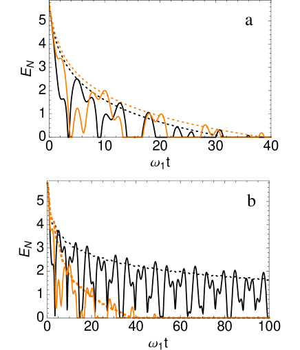
Figure 1: (Color online). Time evolution of an entangled two-mode squeezed initial state (10) with $r=2$, in the case of a) separate baths and b) common bath. The parameters are $k_{B}T=10\omega_{1}$, $\gamma=0.001\omega_{1}$, and cutoff frequency $\Lambda=50\omega_{1}$. The four curves correspond to the points in figures 2 and 4, namely A(dotted black), B(solid black),C(dotted orange) and D(solid orange). Two features are apparent: in presence of a nonzero coupling $\lambda$ (continuous lines) entanglement oscillates strongly, and second, in the case of separate baths any initial entanglement vanishes fast, while in the case of common bath it can be made to survive by having identical frequencies.

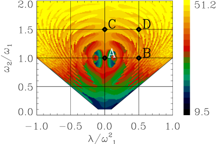
Figure 2: (Color online). Parameter scan of $t_{F}$ (see text) as a function of the oscillators coupling and frequency detuning, in the case of separate baths. We have restricted the scan within a limited detuning ($\omega_{2}\leq 2\omega_{1}$) as a result of the absence of any important features outside this region. In addition, the condition $\lambda<\omega_{1}\omega_{2}$ ensures reality of the eigenfrequencies in the problem. The behavior of $t_{F}$ is basically monotonic in $\omega_{2}/\omega_{1}$, with a superimposed arena-like shape, coming from the oscillatory nature of entanglement. See text for more details. The dots A, B, C, D are given in figure 1 as examples.

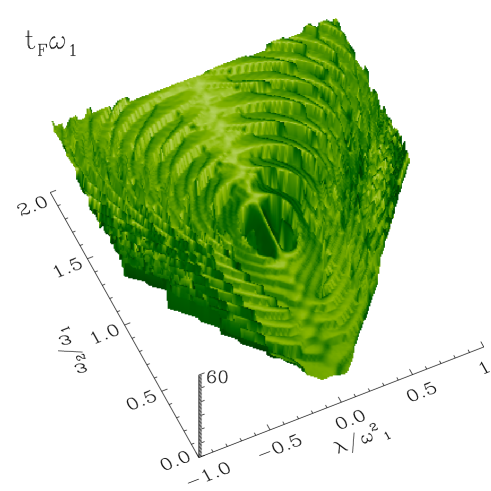
Figure 3: (Color online). Three dimensional representation of figure 2. Here the arena-like shape can be better appreciated.

III.2 Common bath

Let us compare now the previous results with the oscillators evolution with dissipation through a common bath, Eq. (9). This model can be considered a limit case while separate baths would model the opposite one, when baths are completely uncorrelated. The presence of asymptotic entanglement in this situation has been studied by asympt_ent_osc ; paz-roncaglia ; liu , showing that entanglement can survive for sufficiently low temperatures (or conversely for high enough initial squeezings). In the case with different frequencies Paz and Roncaglia noticed in Ref. paz-roncaglia2 that this asymptotic behavior disappears as the detuning is increased, meaning that it is highly dependent on the frequency matching between oscillators and the fact that each oscillator’s bath can be regarded as ‘perfectly correlated’ to the other one. In physical realizations these two conditions will hardly be met and it is interesting to know the effect of deviations from it. We have then studied the effects of frequency diversity in the case of a common bath, looking again at the robustness of entanglement in terms of the decay time $t_{F}$ (Fig.1b). In Fig. 5 we show results equivalent to what represented in Fig. 3 but for common bath. There we see that in the resonant case entanglement never vanishes, and so the survival time is in that case infinite. In Fig. 5 diverging times $t_{F}$ are recognized along the line $\omega_{1}=\omega_{2}$.

When the oscillators frequencies begin to differ, survival diminishes fast to values similar to the uncorrelated baths case. This phenomenon can be understood from the master equation (9). The fact that the coupling to the bath is $\gamma(x_{1}+x_{2})$ establishes that the mode $x_{-}$ remains decoupled at all times, thus keeping its coherence and contributing positively to a nonzero entanglement. If the frequencies are different, that mode gets coupled to $x_{+}$ which is itself coupled to the bath, and its decoherence is transferred to $x_{-}$. This way, both modes are decohered and end up in a thermal state, with no presence of entanglement. Hence the survival time is finite. Because of this, it is worthy to stress the fact that even if the frequency difference is infinitesimal, decoherence will eventually show up, even though it does so in a time inversely proportional to the infitesimum. Thus, increasing the difference in frequencies just exacerbates the transfer velocity of decoherence from mode $x_{+}$ to mode $x_{-}$. This argument evidences how artificial the ‘equal frequencies’ assumption is.

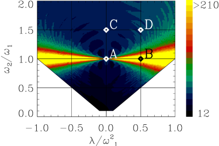
Figure 4: (Color online). Parameter scan of $t_{F}$ (see text) as a function of the oscillators coupling and frequency detuning, in the case of common bath. As seen here, $t_{F}$ is huge whenever the detuning is small, and in the order of tens of periods for high detuning. As expected, at resonance one of the eigenmodes decouples from the baths, leading to an infinite $t_{F}$. We have truncated the plot at heights of $\omega_{1}t_{F}=210$, otherwise this ‘mountain riff’ is infinitely high (but only strictly infinite when $\omega_{1}=\omega_{2}$).

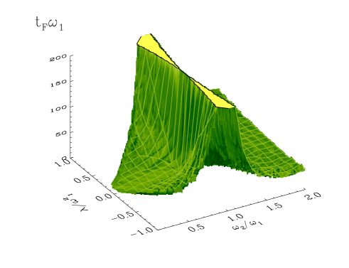
Figure 5: (Color online). 3D representation of Figure 4. Apart from the ‘riff’ at equal frequencies, the shape is very similar to the case of separate baths, with an arena-like bowl shape. We have drawn a mesh to guide the reader’s eye. Again, heights over $t_{F}=210/\omega_{1}$ have been truncated (yellow region).

We point out that asymptotic entanglement can be found also in presence of frequency diversity and is not related to the symmetry present for $\omega_{1}=\omega_{2}$. As a matter of fact, if the couplings to the common bath are different for each oscillator, i.e. $\gamma_{1}\neq\gamma_{2}$, we can restore asymptotic entanglement even off-resonance, for $\omega_{1}\neq\omega_{2}$. By noticing the relation between $x_{1,2}$ with the eigenmodes of the system $Q_{\pm}$, we see that the mode $Q_{+}$ can be uncoupled from the bath when the angle $\theta$ fulfills

$$\cos{\theta}=\frac{\gamma_{1}}{\sqrt{\gamma_{1}^{2}+\gamma_{2}^{2}}}$$ (11)

with $\theta=\theta(\omega_{1},\omega_{2},\lambda)$ given in the Appendix. Thus, half of the system is kept in a pure state, and we can show that entanglement survives asymptotically exactly in the same fashion as it did for equal frequencies above. In other words, with different couplings to the baths together with different frequencies, the system can retain asymptotic entanglement if Eq. (11) is fulfilled. In any case this phenomenon is as unique as the ‘equal frequencies’ one, and requires fine-tuned parameters (tuning bath couplings or frequency difference) in order to be observable. It should then be regarded as exceptional too. Our argument clarifies that asymptotic entanglement is $not$ a consequence of a symmetry in the system, but comes from finely tuned decoherent-free degree of freedom of the system.

III.3 Twin oscillators

We have considered entanglement as an indicator of the quantumness of our system, measurable for the family of (Gaussian) states considered here. The discrimination between the predictions of classical and quantum theories for coupled harmonic oscillators has been largely studied also in optics. In that context there have been many theoretical predictions experimentally confirmed, focusing on the violation of different classical inequalities, or the positivity of variances ineq . An example is the variance of the difference of the occupation numbers:

$$d=\langle:(n_{1}-n_{2})^{2}:\rangle$$ (12)

where, as usual, $n_{i}$ is the occupation number operator of each oscillator. $d$ has been considered in two mode squeezed state generated by parametric oscillators in optics, to characterize twin beams loudon . The quantum character of the correlations in the occupation numbers comes from the negativity of the variance $d$ and can only follow from the negativity of the corresponding quasi-probability, the Glauber-Sudarshan representation in this case. In analogy with the optical case, we consider here $twin$ oscillators looking at the temporal dynamics of $d$. The correspondent fourth order moments can be obtained from the covariance matrix, because the states we are dealing with are Gaussian. In Fig. 6 we plot two examples comparing the evolution of this variance and entanglement for the common/separate baths cases. We have taken only the negative part of this correlation -identifying quantum behavior- and inverted it (plotting $\max(0,-d)$ ) for ease of comparison with entanglement. For the initial entangled state (10), $d=-2\mu/(1-\mu)$, always negative. In other words, for squeezed states the occupation number of one oscillator determines the other one. We observe that starting from this value $d$ decays with large oscillations and that the sudden deaths of entanglement and of this correlation coincide up to a fraction of a period. Still entanglement evolution is smoother and twin oscillators temporarily loose their quantum correlations even for entangled oscillators.

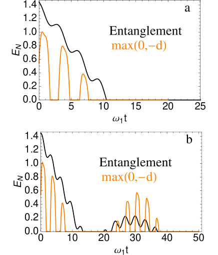
Figure 6: (Color online). Comparison between the time evolutions of entanglement (black) and the correlation measure $\rm{max}(0,-\langle:(n_{1}-n_{2})^{2}:\rangle$) (orange), for the case of a) separate baths and b) common bath. We have used equal frequencies, coupling $\lambda=0.1\omega_{1}^{2}$, damping $\gamma=0.001\omega_{1}$, temperature $k_{B}T/\omega_{1}=10$ and initial squeezing parameter $r=0.5$. The envelope of the correlation measure seems to be closely related to the entanglement, except for a delay of half a period.

IV Non-Markovian evolution

Up to now we have considered the Markovian master equation, in the sense that the time-dependent coefficients related to the heat bath have been replaced by their asymptotic value, obtained by integrating up to infinite time. This implies a complete absence of memory in the bath, which does not retain instantaneous information on the dynamics of the two oscillators. However, this simplification can be dropped, and we are left with a complete description within the weak coupling approximation. In this section we analyze how these corrections affect the entanglement evolution we discussed so far.

In Ref. maniscalco , a comparison has been made considering temperatures two orders of magnitude greater than the frequency cut-off. The authors found that, when the frequency of the oscillators falls inside the bath spectral density, entanglement persists for a longer time than in a Markovian channel. When there is no resonance between reservoir and oscillators, non-Markovian correlations accelerate decoherence and generate entanglement oscillations.

As it is known, when all the important frequencies are much lower than the cut-off, the density of states of Eq. (6) is expected to generate almost memoryless friction weiss . Then, taking $\omega_{1}\ll\Lambda$, we compared Markovian and non-Markovian entanglement dynamics for different choices of the parameters of the system and the bath ($\omega_{2}/\omega_{1}$, $\lambda/\omega_{1}^{2}$, $\gamma/\omega_{1}$, $k_{B}T/\omega_{1}$, $r$). The following considerations are valid for separate baths as well as for a common environment. In the case of very small coupling ($\gamma\sim 10^{-3}\omega_{1}$) non-Markovian corrections are practically unobservable independently on the value of the system parameters up to relevant temperatures. To observe some appreciable deviations, we need to reach temperatures of the order of $10\omega_{1}$. This result is understood considering that for small values of the system-bath coupling the role played by the bath itself is highly reduced. Since non-Markovian corrections to the values of the coefficients are relevant only during the first stage of the evolution, it can be also predicted that if the initial state is robust enough (as, for instance, in the case of squeezing $r=2$ discussed in the previous sections), non-Markovianity will have marginal effects. It is in fact true that, in the case of $\gamma\sim 10^{-3}\omega_{1}$ and $T\sim 10\omega_{1}$, a correction to the entanglement decay time can only be observed assuming low initial squeezing ($r\lesssim 0.1$). When $\gamma$ starts to increase, it is possible to deal with cases where some observable corrections due to non-Markovianity emerge also in the low-temperature regime. In particular, the case of equal frequencies turns out to be the more sensitive. To give an example, in Fig. 7 we compared the two evolutions for two different values of $r$. Starting from $r=2$, non-Markovian corrections are almost negligible, giving corrections of few percents to the value of $t_{F}$ found within the Markovian approximation. In order to observe a noticeable difference, we must start with a factorized state ($r=0$). As it can be observed in Fig. 7, in this case, while memoryless baths are able to support a very small quantity of entanglement, the initial kick given by non-Markovian coefficients enhances entanglement generation, its maximum amount is amplified of about one order of magnitude, and also its death time is increased. It is however worth noting that the absolute value reached is, in any case, very low.

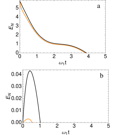
Figure 7: (Color online). Comparison between Markovian (orange) and non-Markovian (black) entanglement dynamics. The system parameters are $\omega_{1}=\omega_{2}$, $\lambda=0.2\omega_{1}^{2}$, $\gamma=0.01\times 2/\pi\omega_{1}$, $\Lambda=20\omega_{1}$, and $k_{B}T=10\omega_{1}$. The initial squeezings are a) $r=2$ and b) $r=0$.

V Discussion and conclusion

During last years, a series of papers has investigated entanglement dynamics of coupled harmonic oscillators in contact with thermal environments. Nevertheless, a comprehensive analysis around the role played by the diversity of the two oscillators was missing.

We started our discussion with the case of separate baths, which seems to be more physically meaningful. As one should expect, after a transient, unless the temperature is very low, the initial two-mode squeezed state $|\Psi_{TMS}\rangle$ becomes separable. Studying the decay time, we observed a series of interesting features that we have qualitatively explained. First of all, by increasing $\omega_{2}/\omega_{1}$ and by keeping unchanged all other parameters, entanglement survival time increases as well. In the limit of $\omega_{2}/\omega_{1}\gg 1$, $\Omega_{+}$ and $\Omega_{-}$ tend, respectively, to $\omega_{2}$ and $\omega_{1}$. Since the asymptotic thermal state the system is reaching depends itself on the frequencies, the purity of the final state is enhanced together with the coherence time necessary to reach it. On the other hand, near $\omega_{2}=\omega_{1}$, entanglement survival time can be raised also by increasing $|\lambda|$. When $|\lambda|\rightarrow\omega_{1}^{2}$, $\Omega_{-}$ is close to zero. Here, we argue that the behavior we observe is the result of two competing effects. If, on one side, the thermal equilibrium state is less pure because of the presence of a vanishing frequency, on the other side, the number of decohering channels goes to zero, since $\Omega_{-}$ falls in a poorly populated region of the spectral density, increasing in this way the time necessary to reach the thermal equilibrium.

If the two oscillators share a common bath, it becomes possible the observation of asymptotic entanglement at relevant temperatures. One of the two eigenmodes of the system can result in fact decoupled from the environment. As a consequence of this decoupling, the asymptotic density matrix will result as the direct sum of the matrix of pure state and of a thermal state, corresponding to the mode interacting with the bath. When the two oscillators have identical frequencies and bath couplings, the mode $x_{-}$ gets decoupled independently of the value of $\lambda$, giving rise to the plateau we observe in Figs. 4, 5. It is important to stress that this regime can be achieved not only when the oscillators are resonant, but also in presence of frequency detuning, through a proper engineering of the system-bath interaction. Conversely, if their bath couplings are different $\gamma_{1}\neq\gamma_{2}$, frequencies $\omega_{1}$ and $\omega_{2}$ can be found so that this special regime is achieved.

We also studied the dynamical evolution of the degree of quantumness of the system by means of the quantity $d$, introduced in Eq. (12). The negativity of this quantity is a direct evidence of the negativity of the Glauber-Sudarshan quasi-probability distribution of the state. The agreement between the behavior of $d$ and the entanglement is worth to be investigated, since a tight relation between them is not known.

As for the Markovian versus non-Markovian debate, we compared the two behaviors in a wide range of parameters. While in Ref. maniscalco the authors investigated what changes when the frequency of the oscillators goes outside from the spectral distribution of the bath in the high temperature regime, we tried to do an extensive analysis for $\omega_{1},\omega_{2}\ll\Lambda$. Our results indicate that non-Markovian corrections can be observed, and are important, only for a reduced subset of initial conditions. To see them, we must put a relevant coupling between oscillators and bath, $\omega_{1}$ should be close to $\omega_{2}$, and the initial state should be (almost) disentangled. Since the master equation has been obtained in the weak-coupling limit, the first of this assumptions seems at least questionable. If we release only one of them, Markovian and non-Markovian evolutions are almost identical.

Appendix A Derivation of master equation

A system-bath model is usually described through the Hamiltonian $H=H_{S}+H_{B}+V$, where $H_{S}$ refers to the system and $H_{B}$ to the bath, and where $V$ is the term containing the interaction. Generally, the coupling term can be written as $V=\sum_{k}S_{k}\otimes B_{k}$, where $S_{k}$ denote system operators and $B_{k}$ bath operators. The master equation for the reduced density matrix to the second order in the coupling strength (for a general discussion see for instance gardiner ) is given by

$$\frac{d\rho}{dt} = -i[H_{S},{\rho}]$$ (13)

$$- \int_{0}^{t}d\tau\sum_{l,m}\big{\{}C_{l,m}(\tau)[S_{l}\tilde{S}_{m}(-\tau)\rho-\tilde{S}_{m}(-\tau)\rho S_{l}]$$

$$+ C_{m,l}(-\tau)[\rho\tilde{S}_{m}(-\tau)S_{l}-S_{l}\rho\tilde{S}_{m}(-\tau)]\big{\}}.$$

Here, $C_{l,m}(\tau)$ are the bath’s correlation functions, defined by

$$C_{l,m}(\tau)={\rm Tr}_{B}[\tilde{B}_{l}(\tau)\tilde{B}_{m}(0)R_{0}],$$ (14)

being $R_{0}=\left(e^{-\beta H_{B}}/{\rm Tre^{-\beta H_{B}}}\right)$ the equilibrium density matrix of the bath. In Eqs. (13,14) the tilde indicates the interaction picture taken with respect to $H_{0}=H_{S}+H_{B}$. For instance, $\tilde{B}_{l}(\tau)=e^{iH_{0}\tau}B_{l}e^{-iH_{0}\tau}$.

In the following, the correlation functions will appear combined as $C_{l,m}^{A}(\tau)=C_{l,m}(\tau)+C_{m,l}(-\tau)$ and $C_{l,m}^{C}(\tau)=C_{l,m}(\tau)-C_{m,l}(-\tau)$.

A.1 Separate baths

In our model, whose Hamiltonian is $H^{sep}$, we can identify $B_{1}=\sum_{k}\lambda_{k}^{(1)}X_{k}^{(1)}$ and $B_{2}=\sum_{k}\lambda_{k}^{(2)}X_{k}^{(2)}$ and, correspondingly, $S_{1}=x_{1},S_{2}=x_{2}$ . Their expressions in the interaction picture are

$$\tilde{B}_{i}=\sum_{k}\lambda_{k}^{(i)}\left[X_{k}^{(i)}\cos\Omega_{k}^{(i)}t+P_{k}^{(i)}\dfrac{\sin\Omega_{k}^{(i)}t}{m\Omega_{k}^{(i)}}\right]$$ (15)

and $\tilde{x}_{i}(\tau)=\alpha_{i1}x_{1}+\alpha_{i2}x_{2}+\beta_{i1}p_{1}+\beta_{i2}p_{2}$, with

$$\alpha_{11} = \cos^{2}\theta\cos\Omega_{-}\tau+\sin^{2}\theta\cos\Omega_{+}\tau,$$ (16)

$$\alpha_{12} = \frac{\sin 2\theta}{2}(\cos\Omega_{+}\tau-\cos\Omega_{-}\tau),$$ (17)

$$\beta_{11} = \frac{\cos^{2}\theta}{\Omega_{-}}\sin\Omega_{-}\tau+\frac{\sin^{2}\theta}{\Omega_{+}}\sin\Omega_{+}\tau,$$ (18)

$$\beta_{12} = \frac{\sin 2\theta}{2}(\frac{\sin\Omega_{+}\tau}{\Omega_{+}}-\frac{\sin\Omega_{-}\tau}{\Omega_{-}}),$$ (19)

and $\alpha_{22}(\theta)=\alpha_{11}(\pi/2-\theta)$, $\beta_{22}(\theta)=\beta_{11}(\pi/2-\theta)$, $\alpha_{21}=\alpha_{12}$, and $\beta_{21}=\beta_{12}$. The coefficients appearing in Eqs. (16-19) are defined as

$$\theta=\frac{1}{2}\arctan\left(\frac{2\lambda}{\omega_{2}^{2}-\omega_{1}^{2}}\right)$$ (20)

and

$$\Omega_{\pm}=\sqrt{\frac{\omega_{1}^{2}+\omega_{2}^{2}}{2}\pm\frac{\sqrt{4\lambda^{2}+(\omega_{2}^{2}-\omega_{1}^{2})^{2}}}{2}}.$$ (21)

The normal modes for the position are

$$Q_{+}=\cos\theta x_{2}+\sin\theta x_{1},$$ (22)

$$Q_{-}=\cos\theta x_{1}-\sin\theta x_{2},$$ (23)

while for the momentum

$$P_{+}=\cos\theta p_{2}+\sin\theta p_{1},$$ (24)

$$P_{-}=\cos\theta p_{1}-\sin\theta p_{2}.$$ (25)

Notice that, for $\omega_{1}=\omega_{2}$, $\theta=\pi/4$. This implies $\alpha_{11}=\alpha_{22}$ and $\beta_{11}=\beta_{22}$.

Since the two baths are identical and uncorrelated, we have $C_{1,1}(\tau)=C_{2,2}(\tau)=C(\tau)$ and $C_{1,2}(\tau)=C_{2,1}(\tau)=0$. From the knowledge of the density of states $J(\Omega)$ it is possible to obtain the explicit expression of $C^{C}(\tau)$ and $C^{A}(\tau)$:

$$C^{C}(\tau) = -i\int_{0}^{\infty}d\Omega J(\Omega)\sin\Omega\tau,$$ (26)

$$C^{A}(\tau) = \int_{0}^{\infty}d\Omega J(\Omega)\cos\Omega\tau\coth\frac{\Omega}{2k_{B}T}.$$ (27)

The master equation reads

$$\frac{d\rho}{dt} = -i[H_{S},{\rho}]-\int_{0}^{t}d\tau\sum_{i=1,2}\big{\{}[x_{i},\{x_{i}(-\tau),\rho\}]\frac{C^{C}(\tau)}{2}$$ (28)

$$+ [x_{i},[x_{i}(-\tau),\rho]]\frac{C^{A}(\tau)}{2}\big{\}}.$$

By using expressions (16-19), it can be written as in Eq. (4), with

$$\epsilon_{ij}^{2} = -i\int_{0}^{t}d\tau\alpha_{ij}C^{C}(\tau),$$ (29)

$$D_{ij} = \int_{0}^{t}d\tau\alpha_{ij}C^{A}(\tau),$$ (30)

$$F_{ij} = \int_{0}^{t}d\tau\beta_{ij}C^{A}(\tau),$$ (31)

$$\Gamma_{ij} = i\int_{0}^{t}d\tau\beta_{ij}C^{C}(\tau).$$ (32)

The considerations about symmetry given in Sec. II can be understood in terms of the explicit form of the master equation. The substitution $\lambda\rightarrow-\lambda$ is equivalent to sending $\theta$ to $-\theta$. Then, also $\alpha_{12}$ and $\beta_{12}$ change their sign. But, since these coefficients multiply one operator (position or momentum) of the first oscillator and one operator of the second one, the canonical transformation $U$ compensates the change of sign, and the evolution of $\rho$ is unchanged.

The explicit form of $\epsilon_{ij},D_{ij},\Gamma_{ij},F_{ij}$, in the Markovian case, can be calculated using the equalities

$$\lim_{t\rightarrow\infty}\int_{0}^{t}d\tau e^{-i(\omega-\omega_{0})\tau}=\pi\delta(\omega-\omega_{0})+i\frac{P}{\omega-\omega_{0}},$$ (33)

where $P$ denotes the Cauchy principal value, and

$$\coth{\frac{\omega}{2k_{B}T}}=2k_{B}T\sum_{n=-\infty}^{+\infty}\frac{\omega}{\omega^{2}+\nu_{n}^{2}},$$ (34)

with $\nu_{n}=2\pi nk_{B}T$.

From the master equation, a set of closed equations of motion for the average values of the second moments can be derived ($i,j=1,2$):

$$\frac{d\langle x_{i}x_{j}\rangle}{dt} = \langle p_{i}x_{j}+p_{j}x_{i}\rangle$$ (35)

$$\frac{d\langle p_{i}p_{j}\rangle}{dt} = -\frac{1}{2}(\omega_{i}^{2}+\epsilon_{ii}^{2})\langle\{x_{i},p_{j}\}\rangle-\frac{1}{2}(\omega_{j}^{2}+\epsilon_{jj}^{2})\langle\{x_{j},p_{i}\}\rangle$$ (36)

$$- \frac{1}{2}(\lambda+\epsilon_{12}^{2})\sum_{k=1}^{2}[\langle\{x_{k},p_{i}\}\rangle(1-\delta_{k,j})+\langle\{x_{k},p_{j}\}\rangle(1-\delta_{k,i})]$$

$$- (\Gamma_{ii}+\Gamma_{jj})\langle p_{i}p_{j}\rangle-\Gamma_{12}\sum_{k=1}^{2}[\langle p_{k}p_{i}\rangle(1-\delta_{k,j})+\langle p_{k}p_{j}\rangle(1-\delta_{k,i})]+D_{ij}$$

$$\frac{d\langle\{x_{i},p_{j}\}\rangle}{dt} = 2\langle p_{i}p_{j}\rangle-2(\omega_{j}^{2}+\epsilon_{jj}^{2})\langle x_{i}x_{j}\rangle-2(\lambda+\epsilon_{12}^{2})\left[\langle x_{i}^{2}\rangle(1-\delta_{ij})+\delta_{ij}\langle x_{1}x_{2}\rangle\right]$$ (37)

$$- \Gamma_{jj}\langle\{x_{i},p_{j}\}\rangle-\Gamma_{12}\langle\{x_{i},p_{i}\}\rangle+F_{ij}$$

A.2 Common bath

In this case, $C_{1,1}(\tau)=C_{2,2}(\tau)=C_{1,2}(\tau)=C_{2,1}(\tau)$. Then, the master equation can be written as has

$$\frac{d\rho}{dt} = -i[H_{S},{\rho}]-\int_{0}^{t}d\tau\sum_{i,j=1,2}\big{\{}[x_{i},\{x_{j}(-\tau),\rho\}]\frac{C^{C}(\tau)}{2}$$ (38)

$$+ [x_{i},[x_{j}(-\tau),\rho]]\frac{C^{A}(\tau)}{2}\big{\}}.$$

and, using Eqs. (29-32), assumes the form given in Eq. (9) with $\bar{D}_{ii}=D_{ii}+D_{12}$ and similarly for $\epsilon^{2},\Gamma,F$. The equations of motion for the second moments read ($i,j=1,2$)

$$\frac{d\langle x_{i}x_{j}\rangle}{dt} = \langle p_{i}x_{j}+p_{j}x_{i}\rangle$$ (39)

$$\frac{d\langle p_{i}p_{j}\rangle}{dt} = -\sum_{k=1}^{2}(\omega_{k}^{2}+\bar{\epsilon}_{kk}^{2})(\langle x_{k}p_{j}\rangle\delta_{ik}+\langle p_{i}x_{k}\rangle\delta_{jk})$$ (40)

$$- \frac{1}{2}\sum_{k=1}^{2}(\lambda+\bar{\epsilon}_{ii}^{2})\left[\langle\{x_{k},p_{i}\}\rangle(1-\delta_{kj})+\langle\{x_{k},p_{j}\}\rangle(1-\delta_{ki})\right]+\frac{1}{2}(\bar{D}_{ii}+\bar{D}_{jj})$$

$$- (\bar{\Gamma}_{ii}+\bar{\Gamma}_{jj})\langle p_{i}p_{j}\rangle-\sum_{k=1}^{2}\bar{\Gamma}_{kk}[\langle p_{i}p_{k}\rangle(1-\delta_{kj})+\langle p_{j}p_{k}\rangle(1-\delta_{ki})]$$

$$\frac{d\langle\{x_{i},p_{j}\}\rangle}{dt} = 2\langle p_{1}p_{2}\rangle-2(\omega_{j}^{2}+\bar{\epsilon}_{jj}^{2})\langle x_{i}x_{j}\rangle$$

$$- 2\sum_{k=1}^{2}(\lambda+\bar{\epsilon}_{kk}^{2})\langle x_{i}x_{k}\rangle(1-\delta_{ik})\delta_{ij}-2(\lambda+\bar{\epsilon}_{ii}^{2})\langle x_{i}^{2}\rangle(1-\delta_{ij})$$

$$- \bar{\Gamma}_{jj}\langle\{x_{i},p_{j}\}\rangle-\sum_{k=1}^{2}\bar{\Gamma}_{kk}\langle\{x_{i},p_{k}\}\rangle(1-\delta_{ik})+\bar{F}_{ii}$$

References

- (1) R. Loudon, The Quantum Theory of Light, (Oxford University Press, 2000).
- (2) S. Haroche, J.-M. Raimond, Exploring the Quantum: Atoms, Cavities, and Photons, (Oxford University Press, USA, 2006).
- (3) A. Naik et al., Nature 443, 193 (2006).
- (4) T. Rocheleau, T. Ndukum, C. Macklin, J. B. Hertzberg, A. A. Clerk, K. C. Schwab, Nature 463, 72 (2010) .
- (5) F. Marquardt, S. M. Girvin, Physics 2, 40 (2009) and references therein;, A. Schliesser et al. Nature Phys. 5, 509 (2009); Y.-S. Park and H. Wang, Nature Phys. 5, 489 (2009), S. Groblacher et al. Nature Phys. 5, 485 (2009).
- (6) L. Amico, R. Fazio, A. Osterloh, and V. Vedral, Rev. Mod. Phys. 80, 517 (2008).
- (7) M. Srednicki, Phys. Rev. Lett. 71, 666 (1993); K. Audenaert, J. Eisert, M. B. Plenio, and R. F. Werner, Phys. Rev. A 66, 042327 (2002); M. B. Plenio, J. Hartley and J. Eisert, New J. Phys. 6, 36 (2004); R. G. Unanyan and M. Fleischhauer, Phys. Rev. Lett. 95, 260604 (2005).
- (8) J. Eisert, M.B. Plenio, S. Bose, J. Hartley, Phys. Rev. Lett. 93, 190402 (2004).
- (9) F. Galve and E. Lutz, Phys. Rev. A, 79, 032327 (2009).
- (10) K.-L. Liu and H.-S. Goan, Phys. Rev. A 76, 022312 (2007).
- (11) J. P. Paz and A. J. Roncaglia, Phys. Rev. Lett. 100, 220401 (2008).
- (12) J. P. Paz and A. J. Roncaglia, Phys. Rev. A 79, 032102 (2009).
- (13) R. Simon, Phys. Rev. Lett. 84, 2726 (2000).
- (14) G. Vidal and R. F. Werner, Phys. Rev. A 65, 032314 (2002).
- (15) K. Zyczkowski, P. Horodecki, A. Sanpera and M. Lewenstein, Phys. Rev. A 58, 883 (1998).
- (16) C. K. Hong, Z. Y. Ou, and L. Mandel, Phys. Rev. Lett. 59, 2044 (1987).
- (17) C. Santori, D. Fatta, J. Vucaronkovic, G S. Solomon, Y. Yamamoto, Nature 419, 594-597 (2002).
- (18) A. J. Bennett, R. B. Patel, C. A. Nicoll, D. A. Ritchie, and A. J. Shields, Nature Phys. 5, 715 (2009) .
- (19) P. D. Drummond, Z. Ficek, Quantum squeezing, (Springer, 2004).
- (20) S. L. Braunstein and P. van Loock, Rev. Mod. Phys. 77, 513 (2005).
- (21) P. Leaci, and A. Ortolan, Phys. Rev. A 76, 062101 (2007).
- (22) S. Gröblacher, K. Hammerer, M. R. Vanner, M. Aspelmeyer, Nature 460, 724 (2009) .
- (23) J. Anders, Phys. Rev. A 77, 062102 (2008) .
- (24) See review T. Yu, J. H. Eberly, Science 323, 598 (2009) and references therein.
- (25) J. S. Prauzner-Bechcicki, J. Phys. A 37, L173 (2004).
- (26) M. Schlosshauer, Decoherence and the Quantum-to-Classical Transition (Springer, Berlin 2007); X.L. Feng, C.J.White, A. Hajimiri, M.L. Roukes, Nature Nanotechnology 3, 342 (2008); T.J. Kippenberg, K.J. Vahala, Science 321, 1172 (2008).
- (27) S. Maniscalco, S. Olivares, and M. G. A. Paris, Phys. Rev. A 75, 062119 (2007).
- (28) T. Zell, F. Queisser, and R. Klesse, Phys. Rev. Lett 102, 160501 (2009).
- (29) A.O. Caldeira and A.J. Leggett, Physica 121A, 587 (1983).
- (30) A. Peres, Phys. Rev. Lett. 77, 1413 (1996).
- (31) M. Horodecki, P. Horodecki, and R. Horodecki, Phys. Lett. A 223, 1 (1996).
- (32) A. Einstein, B. Podolsky, and N. Rosen, Phys. Rev. 47, 777 (1935).
- (33) G. Adesso, A. Serafini, and F. Illuminati, Phys. Rev. Lett. 92, 087901 (2004) .
- (34) G. Giorgi, F. Galve, R. Zambrini, in preparation.
- (35) M. D. Reid and D. F. Walls, Phys. Rev. A 34, 1260 (1986)
- (36) U. Weiss, Quantum Dissipative Systems (World Scientific, Singapore, 1999).
- (37) C. W. Gardiner and P. Zoller, Quantum Noise (Springer, Berlin, 2000).