The Thurston metric on hyperbolic domains and boundaries of convex hulls

Abstract.

We show that the nearest point retraction is a uniform quasi-isometry from the Thurston metric on a hyperbolic domain $\Omega\subset\hat{\mathbb{C}}$ to the boundary ${\rm Dome}(\Omega)$ of the convex hull of its complement. As a corollary, one obtains explicit bounds on the quasi-isometry constant of the nearest point retraction with respect to the Poincaré metric when $\Omega$ is uniformly perfect. We also establish Marden and Markovic’s conjecture that $\Omega$ is uniformly perfect if and only if the nearest point retraction is Lipschitz with respect to the Poincaré metric on $\Omega$.

1. Introduction

In this paper we continue the investigation of the relationship between the geometry of a hyperbolic domain $\Omega$ in $\hat{\mathbb{C}}$ and the geometry of the boundary ${\rm Dome}(\Omega)$ of the convex core of its complement. The surface ${\rm Dome}(\Omega)$ is hyperbolic in its intrinsic metric ([15, 30]) and the nearest point retraction $r:\Omega\to{\rm Dome}(\Omega)$ is a conformally natural homotopy equivalence. Marden and Markovic [25] showed that, if $\Omega$ is uniformly perfect, the nearest point retraction is a quasi-isometry with respect to the Poincaré metric on $\Omega$ and the quasi-isometry constants depend only on the lower bound for the injectivity radius of $\Omega$ in the Poincaré metric.

In this paper, we show that the nearest point retraction is a quasi-isometry with respect to the Thurston metric for any hyperbolic domain $\Omega$ with quasi-isometry constants which do not depend on the domain. We recover, as corollaries, many of the previous results obtained on the relationship between a domain $\Omega$ and ${\rm Dome}(\Omega)$ and obtain explicit constants for the first time in several cases. We also see that the nearest point retraction is Lipschitz if and only if the domain is uniformly perfect, which was originally conjectured by Marden and Markovic [25].

We will recall the definition of the Thurston metric in section 3. It is 2-bilipschitz (see Kulkarni-Pinkall [23]) to the perhaps more familiar quasihyperbolic metric originally defined by Gehring and Palka [20]. Recall that if $\Omega\subset\mathbb{C}$ and $\delta(z)$ denotes the Euclidean distance from $z\in\Omega$ to $\partial\Omega$, then the quasihyperbolic metric is simply $q(z)={1\over\delta(z)}dz$. The Thurston metric has the advantage of being conformally natural, i.e. invariant under conformal automorphisms of $\Omega$.

Theorem 1.1.

Let $\Omega\subset\hat{\mathbb{C}}$ be a hyperbolic domain. Then the nearest point retraction $r:\Omega\rightarrow{\rm Dome}(\Omega)$ is 1-Lipschitz and a $(K,K_{0})$-quasi-isometry with respect to the Thurston metric $\tau$ on $\Omega$ and the intrinsic hyperbolic metric on ${\rm Dome}(\Omega)$, where $K\approx 8.49$ and $K_{0}\approx 7.12$. In particular,

$$d_{{\rm Dome}(\Omega)}(r(z),r(w))\leq d_{\tau}(z,w)\leq K\ d_{{\rm Dome}(\Omega)}(r(z),r(w))+K_{0}.$$

Furthermore, if $\Omega$ is simply connected, then

$$d_{{\rm Dome}(\Omega)}(r(z),r(w))\leq d_{\tau}(z,w)\leq K^{\prime}\ d_{{\rm Dome}(\Omega)}(r(z),r(w))+K^{\prime}_{0}.$$

where $K^{\prime}\approx 4.56$ and $K^{\prime}_{0}\approx 8.05$.

Marden and Markovic’s [25] proof that the nearest point retraction is a quasi-isometry in the Poincaré metric if $\Omega$ is uniformly perfect does not yield explicit bounds, as it makes crucial use of a compactness argument. Combining Theorem 1.1 with work of Beardon and Pommerenke [3], which explains the relationship between the Poincaré metric and the quasihyperbolic metric, we obtain explicit bounds on the quasi-isometry constants. We recall that $\Omega$ is uniformly perfect if and only if there is a lower bound for the injectivity radius of $\Omega$ in the Poincaré metric.

Corollary 1.2.

Let $\Omega$ be a uniformly perfect domain in $\hat{\mathbb{C}}$ and let $\nu>0$ be a lower bound for its injectivity radius in the Poincaré metric, then $r:\Omega\to{\rm Dome}(\Omega)$ is $2\sqrt{2}(k+{\pi^{2}\over 2\nu})$-Lipschitz and a $(2\sqrt{2}(k+{\pi^{2}\over 2\nu}),K_{0})$-quasi-isometry with respect to the Poincaré metric. In particular,

$${1\over 2\sqrt{2}(k+{\pi^{2}\over 2\nu})}\ d_{{\rm Dome}(\Omega)}(r(z),r(w))\leq d_{\rho}(z,w)\leq K\ d_{{\rm Dome}(\Omega)}(r(z),r(w))+K_{0}$$

for all $z,w\in\Omega$ where $k=4+\log(2+\sqrt{2})$.

Examples in Section 10, show that the Lipschitz constant cannot have asymptotic form better than $O({1\over|\log\nu|\ \nu})$ as $\nu\to 0$.

When $\Omega$ is simply connected, we obtain:

Corollary 1.3.

Let $\Omega$ be a simply connected domain in $\hat{\mathbb{C}}$. Then

$${1\over 2}\ d_{{\rm Dome}(\Omega)}(r(z),r(w))\leq d_{\rho}(z,w)\leq K^{\prime}\ d_{{\rm Dome}(\Omega)}(r(z),r(w))+K^{\prime}_{0}$$

for all $z,w\in\Omega$.

In particular, this gives a simple reproof of Epstein, Marden and Markovic’s [16] result that the nearest point retraction is 2-Lipschitz. It only relies on the elementary fact that $r$ is 1-Lipschitz (see Lemma 5.2) with respect to the Thurston metric and a result of Herron, Ma and Minda [21] concerning the relationship between the Thurston metric and the Poincaré metric in the simply connected setting.

Marden and Markovic [25] also showed that the nearest point retraction is a quasi-isometry (with respect to the Poincaré metric) if and only if $\Omega$ is uniformly perfect. As another corollary of Theorem 1.1 we obtain the following alternate characterization of uniformly perfect domains which was conjectured by Marden and Markovic. Corollaries 1.2 and 1.4 together give an alternate proof of Marden and Markovic’s original characterization.

Corollary 1.4.

The nearest point retraction $r:\Omega\to{\rm Dome}(\Omega)$ is Lipschitz, with respect to the Poincaré metric on $\Omega$ and the intrinsic hyperbolic metric on ${\rm Dome}(\Omega)$ if and only if the set $\Omega$ is uniformly perfect. Moreover, if $\Omega$ is not uniformly perfect, then $r$ is not a quasi-isometry with respect to the Poincaré metric.

Sullivan [28, 15] showed that there exists a uniform $M$ such that if $\Omega$ is simply connected, then there is a conformally natural $M$-quasiconformal map from $\Omega$ to ${\rm Dome}(\Omega)$ which admits a bounded homotopy to the nearest point retraction. (We say that a map from $\Omega$ to ${\rm Dome}(\Omega)$ is conformally natural if it is $\Gamma$-equivariant whenever $\Gamma$ is a group of Möbius transformations preserving $\Omega$.) Epstein, Marden and Markovic [16, 17] showed that the best bound on $M$ must lie strictly between 2.1 and 13.88. While, combining work of Bishop [6] and Epstein-Markovic [18], the best bound of $M$ lies between 2.1 and 7.82 if we do not require the quasiconformal map to be conformally natural.

Marden and Markovic [25] showed that a domain is uniformly perfect if and only if there is a quasiconformal map from $\Omega$ to ${\rm Dome}(\Omega)$ which is homotopic to the nearest point retraction by a bounded homotopy. Moreover, they show that there are bounds on the quasiconformal constants which depend only on a lower bound for the injectivity radius of $\Omega$. We note that again these bounds are not concrete.

In order to use the nearest point retraction to obtain a conformally natural quasiconformal map between $\Omega$ and ${\rm Dome}(\Omega)$ we show that $r$ lifts to a quasi-isometry between the universal cover $\tilde{\Omega}$ of $\Omega$ and the universal cover ${\rm Dome}(\tilde{\Omega})$ of ${\rm Dome}(\Omega)$. Although they do not make this explicit in their paper, this is essentially the same approach taken by Marden and Markovic [25]. We recall that quasi-isometric surfaces need not even be homeomorphic and that even homeomorphic quasi-isometric surfaces need not be quasiconformal to one another. Notice that the quasi-isometry constants for the lift of the nearest point retraction are, necessarily, not as good as those for the nearest point retraction. Examples in Section 10 show that the first quasi-isometry constant of $\bar{r}$ cannot have form better than $O(\nu e^{\pi^{2}\over 2\nu})$ as $\nu\to 0$.

Theorem 1.5.

Suppose that $\Omega$ is a uniformly perfect hyperbolic domain and $\nu>0$ is a lower bound for its injectivity radius in the Poincaré metric. Then the nearest point retraction lifts to a quasi-isometry

$$\tilde{r}:\tilde{\Omega}\to{\rm Dome}(\tilde{\Omega})$$

between the universal cover of $\Omega$ (with the Poincaré metric) and the universal cover of ${\rm Dome}(\Omega)$ with quasi-isometry constants depending only on $\nu$. In particular,

$${1\over 2\sqrt{2}(k+{\pi^{2}\over 2\nu})}\ d_{{\rm Dome}(\tilde{\Omega})}(\tilde{r}(z),\tilde{r}(w))\leq d_{\tilde{\Omega}}(z,w)\leq L(\nu)d_{{\rm Dome}(\tilde{\Omega})}(\tilde{r}(z),\tilde{r}(w))+L_{0}$$

for all $z,w\in\tilde{\Omega}$ where $L(\nu)=O(e^{\pi^{2}\over 2\nu})$ as $\nu\to 0$ and $L_{0}\approx 8.05$.

We then apply work of Douady and Earle [14] to obtain explicit bound on the quasiconformal map homotopic to the nearest point retraction when $\Omega$ is uniformly perfect.

Corollary 1.6.

There exists an explicit function $M(\nu)$ such that if $\Omega$ is uniformly perfect and $\nu>0$ is a lower bound for its injectivity radius in the Poincaré metric, then there is a conformally natural $M(\nu)$-quasiconformal map $\phi:\Omega\to{\rm Dome}(\Omega)$ which admits a bounded homotopy to $r$. Moreover, if $\Omega$ is not uniformly perfect, then there does not exist a bounded homotopy of $r$ to a quasiconformal map.

We will give explicit formulas for $L$ and $M$ in section 9.

The table below summarizes the main results concerning the nearest point retraction in the cases that the domain is simply connected, uniformly perfect and hyperbolic but not uniformly perfect.

	$\Omega$ simply connected	$\Omega$ uniformly perfect	$\Omega$ hyperbolic
		$\mbox{inj}_{\Omega}>\nu$	but not uniformly perfect
Lipschitz bounds on $r$	$r$ is 2-Lipschitz	$r$ is $K(\nu)$-Lipschitz	$r$ is not Lipschitz
in Poincaré metric	(see [16] and Cor. 1.3)	where $K(\nu)=2\sqrt{2}(k+\frac{\pi^{2}}{2\nu})$ $k\approx 5.76$	(Corollary 1.4)
		(Corollary 1.2)
quasi-isometry bounds on $r$	$r$ is a $(K^{\prime},K^{\prime}_{0})$-quasi-isometry	$r$ is a $(K(\nu),K_{0})$-quasi-isometry	$r$ is not a
in Poincaré metric	where $K^{\prime}\approx 4.56$, $K^{\prime}_{0}\approx 8.05$	where $K_{0}\approx 7.12$	quasi-isometry
	(Corollary 1.3)	(Corollary 1.2)	(see [25] and Cor. 1.4)
Lipschitz bounds on r	$r$ is $1$-Lipschitz	$r$ is $1$-Lipschitz	$r$ is $1$-Lipschitz
in Thurston metric	(Theorem 1.1)	(Theorem 1.1)	(Theorem 1.1)
quasi-isometry bounds on $r$	$r$ is a $(K^{\prime},K^{\prime}_{0})$-quasi-isometry	$r$ is a $(K,K_{0})$-quasi-isometry	$r$ is a $(K,K_{0})$-quasi-isometry
in Thurston metric	(Theorem 1.1)	where $K\approx 8.49$	(Theorem 1.1)
		(Theorem 1.1)
conformally natural	$M$-quasiconformal map	$M(\nu)$-quasiconformal map	no quasiconformal map
quasiconformal map	where $2.1<M<13.88$	(Corollary 1.6)	(see [25] and Cor. 1.6)
homotopic to $r$	(see [16] and [17])
by a bounded homotopy
quasiconformal map	$M^{\prime}$-quasiconformal map	$M(\nu)$-quasiconformal map	no quasiconformal map
homotopic to $r$	where $2.1<M^{\prime}<7.82$	(Corollary 1.6)	(see [25] and Cor. 1.6)
by a bounded homotopy	(see [6] and [18])

The only constant in the table above which is known to be sharp is the Lipschitz constant in the simply connected case. It would be desirable to know sharp bounds (or better bounds) in the remaining cases. We refer the reader to the excellent discussion of the relationship between the nearest point retraction and complex analytic problems, especially Brennan’s conjecture, in Bishop [5].

One of the main motivations for the study of domains and the convex hulls of their complements comes from the study of hyperbolic 3-manifolds where one is interested in the relationship between the boundary of the convex core of a hyperbolic manifold and the boundary of its conformal bordification. If $N=\mathbb{H}^{3}/\Gamma$ is a hyperbolic 3-manifold, one considers the domain of discontinuity $\Omega(\Gamma)$ for $\Gamma$’s action on $\hat{\mathbb{C}}$. The conformal boundary $\partial_{c}N$ is the quotient $\Omega(\Gamma)/\Gamma$ and $\hat{N}=N\cup\partial_{c}N$ is the natural conformal bordification of $N$. The convex core $C(N)$ of $N$ is obtained as the quotient of the convex hull of $\hat{\mathbb{C}}-\Omega(\Gamma)$ and its boundary $\partial C(N)$ is the quotient of ${\rm Dome}(\Omega)$. The nearest point retraction descends to a homotopy equivalence

$$\bar{r}:\partial_{c}N\to\partial C(N).$$

In this setting, Sullivan’s theorem implies that if $\partial_{c}N$ is incompressible in $\hat{N}$, then there is a quasiconformal map, with uniformly bounded dilatation, from $\partial_{c}N$ to $\partial C(N)$ which is homotopic to the nearest point retraction.

Since the Thurston metric is $\Gamma$-invariant and the nearest point retraction is $\Gamma$-equivariant we immediately obtain a manifold version of Theorem 1.1.

Theorem 1.7.

Let $N=\mathbb{H}^{3}/\Gamma$ be a hyperbolic 3-manifold. Then the nearest point retraction $r:\partial_{c}N\to C(N)$ is a $(K,K/K_{0})$-quasi-isometry with respect to the Thurston metric $\tau$ on $\partial_{c}N$ and the intrinsic hyperbolic metric on $\partial C(N)$. In particular,

$$d_{\partial C(N)}(\bar{r}(z),\bar{r}(w))\leq d_{\tau}(z,w)\leq K\ d_{\partial C(N)}(\bar{r}(z),\bar{r}(w))+K_{0}.$$

We also obtain a version of Corollary 1.2 in the manifold setting.

Corollary 1.8.

Let $N=\mathbb{H}^{3}/\Gamma$ be a hyperbolic 3-manifold such that there is a lower bound $\nu>0$ for the injectivity radius of $\Omega(\Gamma)$ (in the Poincaré metric), then

$${1\over 2\sqrt{2}(k+{\pi^{2}\over 2\nu})}\ d_{\partial C(N)}(\bar{r}(z),\bar{r}(w))\leq d_{\rho}(z,w)\leq K\ d_{\partial C(N)}(\bar{r}(z),\bar{r}(w))+K_{0}$$

for all $z,w\in\partial_{c}N$ where $k=4+\log(2+\sqrt{2})$.

We also obtain a version of Corollary 1.6 which guarantees the existence of a quasiconformal map from the conformal boundary to the boundary of the convex core.

Corollary 1.9.

If $N=\mathbb{H}^{3}/\Gamma$ is a hyperbolic 3-manifold and $\nu>0$ is a lower bound for the injectivity radius of $\Omega(\Gamma)$ (in the Poincaré metric), then there is a $M(\nu)$-quasiconformal map $\phi:\partial_{c}N\to\partial C(N)$ which admits a bounded homotopy to the nearest point retraction $\bar{r}$.

If $N$ is a hyperbolic 3-manifold with finitely generated fundamental group, then its domain of discontinuity is uniformly perfect (see Pommerenke [27]), so Corollaries 1.8 and 1.9 immediately apply to all hyperbolic 3-manifolds with finitely generated fundamental group. More generally, analytically finite hyperbolic 3-manifolds (i.e. those whose conformal boundary has finite area) are known to be uniformly perfect [12].

We recall that it was earlier shown (see [9]) that the nearest point retraction $\bar{r}:\partial_{c}N\to\partial C(N)$ is $(2\sqrt{2}(k+{\pi^{2}\over 2\nu}))$-Lipschitz whenever $N$ is analytically finite and has a $J(\nu)$-Lipschitz homotopy inverse where $J(\nu)=O(e^{C\over\nu})$ (for some explicit constant $C>0$) as $\nu\to 0$. Moreover, if $N=\mathbb{H}^{3}/\Gamma$ is analytically finite and $\Omega(\Gamma)$ is simply connected, then $\bar{r}$ has a $(1+\frac{\pi}{\sinh^{-1}(1)})$-Lipschitz homotopy inverse. Remark (2) in Section 7 of [9] indicates that one cannot improve substantially on the asymptotic form of the Lipschitz constant for $\bar{r}$ (see also Section 6 of [13]), while Proposition 6.2 of [9] shows that one cannot improve substantially on the asymptotic form of the Lipschitz constant of the homotopy inverse for $\bar{r}$.

Outline of paper: Many of the techniques of proof in this paper are similar to those in our previous papers [8] and [9]. The consideration of the Thurston metric allows us to obtain more general results, while the fact that the Thurston metric behaves well under approximation allows us to reduce many of our proofs to the consideration of the case where $\Omega$ is the complement of finitely many points in $\hat{\mathbb{C}}$ and the convex hull of its complement is a finite-sided ideal polyhedron. Therefore, our techniques are more elementary than much of the earlier work on the subject.

In Section 2 we recall basic facts and terminology concerning the nearest point retraction and the boundary of the convex core. In Section 3 we discuss the Poincaré, quasihyperbolic and Thurston metrics on a hyperbolic domain. In section 4 we establish the key approximation properties which allow us to reduce the proof of Theorems 1.1 and 1.5 to the case where $\hat{\mathbb{C}}-\Omega$ is a finite collection of points. In Section 5 we study the geometry of the finitely punctured case and introduce a notion of intersection number which records the total exterior dihedral angle along a geodesic in ${\rm Dome}(\Omega)$. If $\alpha$ is an arc in ${\rm Dome}(\Omega)$, then the difference between its length and the length of $r^{-1}(\alpha)$ in the Thurston metric is exactly this intersection number, see Lemma 5.2.

Section 6 contains the key intersection number estimates used in the proof of Theorem 1.1. The first estimate, Lemma 6.1, bounds the total intersection numbers of moderate length geodesic arcs in the thick part of ${\rm Dome}(\Omega)$. (Lemma 6.1 is a mild generalization of Lemma 4.3 in [9] and we defer its proof to an appendix.) We then bound the total intersection number of a short geodesic (Lemma 6.6) and the angle of intersection of an edge of ${\rm Dome}(\Omega)$ with a short geodesic (Lemma 6.7). We give a quick proof of a weaker form of Lemma 6.6 and defer the proof of the better estimate to the appendix. In a remark at the end of Section 6, we see that one could use this weaker estimate to obtain a version of Theorem 1.1 with slightly worse constants.

Section 7 contains the proof of Theorem 1.1. It follows immediately from Lemma 5.2 that the nearest point retraction is 1-Lipschitz with respect to the Thurston metric, but it remains to bound the distance between two points $x$ and $y$ in $\Omega$ in terms of the distance between $r(x)$ and $r(y)$ in ${\rm Dome}(\Omega)$. We do so by first dividing the shortest geodesic joining $r(x)$ to $r(y)$ into segments of length roughly $G$ (for some specific constant $G$). The segments in the thick part have bounded intersection number by Lemma 6.1. We use Lemmas 6.6 and 6.7 to replace geodesic segments in the thin part by bounded length arcs which consist of one segment missing every edge and another segment with bounded intersection number. We then obtain a path joining $r(x)$ to $r(y)$ with length and intersection number bounded above by a multiple of $d_{{\rm Dome}(\Omega)}(r(x),r(y))+G$. Lemma 5.2 can then be applied to complete the proof.

In Section 8 we derive consequences of Theorem 1.1, including Corollaries 1.2, 1.3 and 1.4. In Section 9 we prove Theorem 1.5, using techniques similar to those in the proof of Theorem 1.1. We then use work of Douady and Earle [14] to derive Corollary 1.6. In Section 10, we study the special case of round annuli and observe that the asymptotic form of our estimates in Corollary 1.2 and Theorem 1.5 cannot be substantially improved. The appendix, Section 11, contains the complete proofs of Lemmas 6.1 and 6.6. The proof of Lemma 6.1 is considerably simpler than the proof of Lemma 4.3 in [9] as we are working in the finitely punctured case.

2. The nearest point retraction and convex hulls

If $\Omega\subseteq\hat{\mathbb{C}}$ is a hyperbolic domain, we let $CH(\hat{\mathbb{C}}-\Omega)$ be the hyperbolic convex hull of $\hat{\mathbb{C}}-\Omega$ in $\mathbb{H}^{3}$. We then define

$${\rm Dome}(\Omega)=\partial CH(\hat{\mathbb{C}}-\Omega)$$

and recall that it is hyperbolic in its intrinsic metric ([15, 30]). In the special case that $\hat{\mathbb{C}}-\Omega$ lies in a round circle, $CH(\hat{\mathbb{C}}-\Omega)$ is a subset of a totally geodesic plane in $\mathbb{H}^{3}$. In this case, it is natural to consider ${\rm Dome}(\Omega)$ to be the double of $CH(\hat{\mathbb{C}}-\Omega)$ along its boundary (as a surface in the plane).

We define the nearest point retraction

$$r:\Omega\to{\rm Dome}(\Omega),$$

by letting $r(z)$ be the point of intersection of the smallest horosphere about $z$ which intersect ${\rm Dome}(\Omega)$. We note that $r:\Omega\to{\rm Dome}(\Omega)$ is a conformally natural homotopy equivalence. The nearest point retraction extends continuously to a conformally natural map

$$r:\mathbb{H}^{3}\cup\Omega\to CH(\hat{\mathbb{C}}-\Omega)$$

where $r(x)$ is the (unique) nearest point on $CH(\hat{\mathbb{C}}-\Omega)$ if $x\in\mathbb{H}^{3}$ (see [15]).

We recall that a support plane to ${\rm Dome}(\Omega)$ is a plane $P$ which intersects ${\rm Dome}(\Omega)$ and bounds an open half-space $H_{P}$ disjoint from ${\rm Dome}(\Omega)$. The half-space $H_{P}$ is associated to a maximal open disc $D_{P}$ in $\Omega$. Since $D_{P}$ is maximal, $\partial D_{P}$ contains at least two points in $\partial\Omega$. Therefore, $P$ contains a geodesic $g\in{\rm Dome}(\Omega)$. Notice that $P$ intersects ${\rm Dome}(\Omega)$ in either a single edge or a convex subset of $P$ which we call a face of ${\rm Dome}(\Omega)$. If $z\in\Omega$, then the geodesic ray starting at $r(z)$ in the direction of $z$ is perpendicular to a support plane $P_{z}$ through $r(z)$.

3. The Poincaré metric, the quasihyperbolic metric and the Thurston metric

Given a hyperbolic domain $\Omega$ in $\hat{\mathbb{C}}$ there is a unique metric $\rho$ of constant curvature $-1$ which is conformally equivalent to the Euclidean metric on $\Omega$. This metric $\rho$ is called the Poincaré metric on $\Omega$ and is denoted

$$\rho(z)=\lambda_{\rho}(z)\ dz.$$

Alternatively, the Poincaré metric can be given by defining the length of a tangent vector $v\in T_{x}(\Omega)$ to be the infimum of the hyperbolic length over all vectors $v^{\prime}$ such that there exists a conformal map $f:\mathbb{H}^{2}\rightarrow\hat{\mathbb{C}}$ such that $f(\mathbb{H}^{2})\subset\Omega$ and $df(v^{\prime})=v$.

In [3], Beardon and Pommerenke show that the quasihyperbolic metric and the Poincaré metric are closely related. We recall that, the quasihyperbolic metric on $\Omega\subset\mathbb{C}$ is the conformal metric

$$q(z)=\frac{1}{\delta(z)}\ dz$$

where $\delta(z)$ is the Euclidean distance from $z$ to $\partial\Omega$. They let

$$\beta(z)=\inf\left\{\left|\log{|z-a|\over|z-b|}\right|\ :a\in\partial\Omega,\ b\in\partial\Omega,\ |z-a|=\delta(z)\right\}$$

Alternatively, one can define $\beta(z)=\pi M$ where $M$ is the maximal modulus of an essential round annulus (i.e. one which separates $\hat{\mathbb{C}}-\Omega$) in $\Omega$ whose central (from the conformal viewpoint) circle passes through $z$. We recall that if $A$ is any annulus in $\hat{\mathbb{C}}$, then it is conformal to an annulus of the form $\{z\ |\ {1\over t}<|z|<t\}$ and we define its modulus to be

$${\rm mod}(A)={1\over 2\pi}\log(t^{2}).$$

The central circle of $A$ is the pre-image of the unit circle in $\{z\ |\ {1\over t}<|z|<t\}$.

Theorem 3.1.

(Beardon-Pommerenke [3]) If $\Omega$ is a hyperbolic domain in $\mathbb{C}$, then

$${1\over\sqrt{2}(k+\beta(z))}q(z)\leq\rho(z)\leq{2k+{\pi\over 2}\over k+\beta(z)}q(z)$$

for all $z\in\Omega$, where $k=4+\log(3+2\sqrt{2})\approx 5.76$. Moreover,

$$\rho(z)\leq 2q(z)$$

for all $z\in\Omega$. If $\Omega$ is simply connected, then

$${1\over 2}q(z)\leq\rho(z)\leq 2q(z).$$

Using the fact that the core curves of large modulus essential annuli are short in the Poincaré metric, one sees that a lower bound on the injectivity radius of $\Omega$ gives an explicit bilipschitz equivalence between the Poincaré metric and the quasihyperbolic metric when $\Omega$ is uniformly perfect.

Corollary 3.2.

If $\Omega$ is a uniformly perfect hyperbolic domain and $\nu>0$ is a lower bound for the injectivity radius of $\Omega$ in the Poincaré metric, then

$${1\over\sqrt{2}(k+{\pi^{2}\over 2\nu})}q(z)\leq\rho(z)\leq 2q(z)$$

for all $z\in\Omega$.

Proof.

Corollary 3.3 in [13] asserts that if $\beta(z)\geq M$, then ${\rm inj}_{\Omega}(z)\leq{\pi^{2}\over 2M}$. Therefore, if ${\rm inj}_{\Omega}(z)\geq\nu>0$, then $\beta(z)\leq{\pi^{2}\over 2\nu}$. The result then follows from Theorem 3.1. ∎

Another metric closely related to the quasihyperbolic metric is the Thurston metric. The Thurston metric

$$\tau(z)=\lambda_{\tau}(z)\ dz$$

on $\Omega$ is defined by letting the length of a vector $v\in T_{x}(\Omega)$ be the infimum of the hyperbolic length of all vectors $v^{\prime}\in\mathbb{H}^{2}$ such that there exists a Möbius transformation $f$ such that $f(\mathbb{H}^{2})\subset\Omega$ and $df(v^{\prime})=v$. By definition, the Thurston metric is conformally natural and conformal to the Euclidean metric. Furthermore, by our alternate definition of the Poincaré metric, we have the inequality

(1) $$\rho(z)\leq\tau(z)$$

for all $z\in\Omega$.

The Thurston metric is also known as the projective metric, as it arises from regarding $\Omega$ as a complex projective surface and giving it the metric Thurston described on such surfaces. Kulkarni and Pinkall defined and studied an analogue of this metric in all dimensions and it is also sometimes called the Kulkarni-Pinkall metric. See Herron-Ma-Minda [21], Kulkarni-Pinkall [23], McMullen [26] and Tanigawa [29] for further information on the Thurston metric.

Kulkarni and Pinkall (see Theorem 7.2 in [23]) proved that the Thurston metric and the quasihyperbolic metric are 2-bilipschitz.

Theorem 3.3.

([23]) If $\Omega$ is a hyperbolic domain in $\mathbb{C}$ then

$${1\over 2}\tau(z)\leq q(z)\leq\tau(z).$$

In the simply connected setting, Herron, Ma and Minda (see Theorem 2.1 and Lemma 3.1 in [21]) prove that the Poincaré metric and the Thurston metric are also 2-bilipschitz.

Theorem 3.4.

([21]) If $\Omega$ is a simply connected hyperbolic domain in $\hat{\mathbb{C}}$, then

$${1\over 2}\tau(z)\leq\rho(z)\leq\tau(z).$$

We will make use of the following alternate characterization of the Thurston metric. We note that it is not difficult to derive Theorem 3.3 from this characterization.

Lemma 3.5.

If $\Omega$ is a hyperbolic domain in $\mathbb{C}$, then the Thurston metric $\tau(z)$ on $\Omega$ is given by

$$\tau(z)=\frac{1}{h(z)}\ dz$$

where $h(z)$ is the radius of the maximal horoball $B_{z}$ based at $z$ whose interior misses ${\rm Dome}(\Omega)$.

Proof.

Recall the disk model $\Delta$ for $\mathbb{H}^{2}$ with the metric

$$\rho_{\Delta}(z)=\frac{2}{1-|z|^{2}}\ dz=\lambda_{\Delta}(z)\ dz.$$

By normalizing, we may define the length of a vector $v\in T_{x}(\Omega)$ in the Thurston metric to be the infimum of the length of vectors $v^{\prime}\in T_{0}\Delta$ such that there exists a Möbius transformation $m$ such that $m(\Delta)\subset\Omega$ with $dm_{0}(v^{\prime})=v$. The hyperbolic length of $v^{\prime}$ is then simply $2|v^{\prime}|=\frac{2}{|m^{\prime}(0)|}|v|$. Thus

$$\tau(z)=\inf_{m}\frac{2}{|m^{\prime}(0)|}$$

where the infimum is taken over all Möbius transformations $m$ such that $m(\Delta)\subset\Omega$ and $m(0)=z$.

Given such a Möbius transformation $m$, we let $D_{m}=m(\Delta)$ and let $P_{m}$ be the hyperbolic plane with the same boundary as $D_{m}$. We further let $B_{m}$ be the horoball based at $z$ which is tangent to $P_{m}$. As $D_{m}\subseteq\Omega$, $P_{m}$ does not intersect the interior of the convex hull $CH(\hat{\mathbb{C}}-\Omega)$. Similarly, the interiors of $B_{m}$ and $CH(\hat{\mathbb{C}}-\Omega)$ are disjoint. Let $h_{m}$ be the radius of the horoball $B_{m}$. Notice that $h_{m}\leq h(z)$. Let $n$ be a parabolic Möbius transformation with fixed point $z$, which sends $B_{m}\cap P_{m}$ to the point vertically above $z$. Then, $n$ fixes $B_{m}$ and sends $D_{m}$ to a disk centered at $z$ with radius $2h_{m}$. Therefore, since $n\circ m$ sends a disk of radius $1$ to a disk of radius $2h_{m}$ and sends centers to centers,

$$|n\circ m^{\prime}(0)|=|n^{\prime}(z)m^{\prime}(0)|=2h_{m}.$$

Since $n$ is parabolic and fixes $z$, $|n^{\prime}(z)|=1$, which implies that $|m^{\prime}(0)|=2h_{m}$. Therefore

$$\tau(z)=\inf_{m}\frac{2}{|m^{\prime}(0)|}=\inf_{m}\frac{1}{h_{m}}\geq{1\over h(z)}$$

On the other hand, let $P_{z}$ be the support plane to $r(z)$ which is perpendicular to the geodesic ray joining $r(z)$ to $z$. Then $P_{z}$ is tangent to $B_{z}$ at $r(z)$. Let $D_{z}$ be the (open) disk in $\Omega$ containing $z$ whose boundary agrees with $\partial P_{z}$. If $m$ is a Möbius transformation such that $m(0)=z$ and $m(\Delta)=D_{z}$, then, by the above analysis, $|m^{\prime}(0)|=2h(z)$. It follows that

$$\tau(z)={1\over h(z)}$$

as desired. ∎

4. Finite approximations and the geometry of domains and convex hulls

Given a hyperbolic domain $\Omega$, let $\{x_{n}\}_{n=1}^{\infty}$ be a dense set of points in $\hat{\mathbb{C}}-\Omega$. If $X_{n}=\{x_{1},\ldots,x_{n}\}$, then we call $\{X_{n}\}$ a nested finite approximation to $\hat{\mathbb{C}}-\Omega$. Notice that $\{X_{n}\}$ converges to $\hat{\mathbb{C}}-\Omega$ in the Hausdorff topology on closed subsets of $\hat{\mathbb{C}}$. We let $\Omega_{n}=\hat{\mathbb{C}}-X_{n}$, denote the quasihyperbolic metric on $\Omega_{n}$ by $q_{n}$, and let $r_{n}:\Omega_{n}\rightarrow{\rm Dome}(\Omega_{n})$ be the nearest point retraction. Since $\Omega\subseteq\Omega_{n}$, $q_{n}$ and $r_{n}$ are both defined on $\Omega$. Results of Bowditch [7] imply that $\{CH(X_{n})\}$ converges to $CH(\hat{\mathbb{C}}-\Omega)$ and that $\{{\rm Dome}(\Omega_{n})\}$ converges to ${\rm Dome}(\Omega)$ in the Hausdorff topology on closed subsets of $\mathbb{H}^{3}$.

The following approximation lemma will allow us to reduce the proof of many of our results to the case where $\Omega$ is the complement of finitely many points.

Lemma 4.1.

Let $\{X_{n}\}$ be a nested finite approximation to $\hat{\mathbb{C}}-\Omega$. If, for all $n$, $\Omega_{n}=\hat{\mathbb{C}}-X_{n}$, $q_{n}$ is the quasihyperbolic metric on $\Omega_{n}$, and $p_{n}$ is the Thurston metric on $\Omega_{n}$, then

1. the sequence $\{q_{n}\}$ of metrics converges uniformly on compact subsets of $\Omega$ to the quasihyperbolic metric $q$ on $\Omega$,

2. the sequence $\{\tau_{n}\}$ of metrics converges uniformly on compact subsets of $\Omega$ to the Thurston metric $\tau$ on $\Omega$,

3. the associated nearest point retractions $\{r_{n}:\Omega_{n}\rightarrow{\rm Dome}(\Omega_{n})\}$ converge to the nearest point retraction $r:\Omega\rightarrow{\rm Dome}(\Omega)$ uniformly on compact subsets of $\Omega$,

4. if $z,w\in\Omega$, then {$d_{{\rm Dome}(\Omega_{n})}(r_{n}(z),r_{n}(w))\}$ converges to $d_{{\rm Dome}(\Omega)}(r(z),r(w))$, and

5. if $z\in\Omega$, then

   $$\lim{\rm inj}_{{\rm Dome}(\Omega_{n})}(r_{n}(z))={\rm inj}_{{\rm Dome}(\Omega)}(r(z)).$$

Proof.

Let $\delta_{n}(z)$ denote the distance from $z\in\Omega_{n}$ to $X_{n}$. It is clear that $\{\delta_{n}\}$ converges to $\delta$ uniformly on compact subsets of $\Omega$. Therefore, $\{q_{n}\}$ converges uniformly to $q$ on compact subsets of $\Omega$.

If $z\in\Omega_{n}$, let $B^{n}_{z}$ denote the maximal horoball based at $z$ whose interior is disjoint from $CH(X_{n})$ and whose closure intersects ${\rm Dome}(\Omega_{n})$ at $r_{n}(z)$. Suppose that $\{z_{n}\}\subset\Omega$ converges to $z\in\Omega$. Since $\{CH(X_{n})\}$ converges to $CH(\hat{\mathbb{C}}-\Omega)$, $\{B^{n}_{z_{n}}\}$ converges to a horoball $B$ based at $z$ whose interior is disjoint from $CH(\hat{\mathbb{C}}-\Omega)$ and whose closure intersects ${\rm Dome}(\Omega)$ at $\lim r_{n}(z_{n})$. By definition, $r(z)$ is this intersection point, so $r(z)=\lim r_{n}(z_{n})$. Therefore, $\{r_{n}\}$ converges uniformly to $r$ on $\Omega$, establishing (3). Moreover, applying Lemma 3.5, we see that $\{\tau_{n}(z_{n})\}$ converges to $\tau(z)$, so $\{\tau_{n}\}$ converges uniformly to $\tau$ on $\Omega$, which proves (2).

Suppose that $z,w\in\Omega$. If $\gamma_{n}$ is a path in ${\rm Dome}(\Omega_{n})$ of length

$$l_{n}=d_{{\rm Dome}(\Omega_{n}))}(r_{n}(z),r_{n}(w)),$$

then $\gamma_{n}$ converges, up to subsequence, to a path in ${\rm Dome}(\Omega)$ of length at most $\liminf l_{n}$ joining $r(z)$ to $r(w)$. Therefore,

$$d_{{\rm Dome}(\Omega)}(r(z),r(w))\leq\liminf l_{n}.$$

On the other hand, if $\gamma$ is a path in ${\rm Dome}(\Omega)$ of length $l=d_{\rm Dome}(\Omega)(r(z),r(w))$, then $r_{n}(\gamma)$ is a path of length at most $l$ on ${\rm Dome}(\Omega_{n})$ joining $r_{n}(r(z))$ to $r_{n}(r(w))$. Notice that $\{d_{{\rm Dome}(\Omega_{n})}(r_{n}(r(z)),r_{n}(z))\}$ and $\{d_{{\rm Dome}(\Omega_{n})}(r_{n}(r(w)),r_{n}(w))\}$ both converge to 0, since $\{{\rm Dome}(\Omega_{n})\}$ converges to ${\rm Dome}(\Omega)$. Therefore, $\limsup l_{n}\leq l$. It follows that $\lim l_{n}=l$, establishing (4).

The proof of (5) follows much the same logic as the proof of (4).

∎

5. The geometry of finitely punctured spheres

In this section we consider the situation where $\Omega$ is the complement of finitely many points in $\hat{\mathbb{C}}$. In this case, the convex core $CH(\hat{\mathbb{C}}-\Omega)$ of the complement of $\Omega$ is an ideal hyperbolic polyhedron and its boundary ${\rm Dome}(\Omega)$ consists of a finite number of ideal hyperbolic polygons meeting along edges. We give a precise description of the Thurston metric in this case (Lemma 5.1) and show that $r$ is 1-Lipschitz with respect to the Thurston metric (Lemma 5.2). We also introduce an intersection number for a curve $\alpha:[0,1]\to{\rm Dome}(\Omega)$ which is transverse to all edges and give a formula for the length of its pre-image $r^{-1}(\alpha)$ in the Thurston metric on $\Omega$.

5.1. The Thurston metric in the finitely punctured case

Let $\Omega$ be the complement of a finite set in $\hat{\mathbb{C}}$. Each face $F$ of the polyhedron $CH(\hat{\mathbb{C}}-\Omega)$ is contained in a unique plane $P_{F}$. Furthermore, $P_{F}$ bounds a unique open half-space $H_{F}$ which does not intersect $CH(\hat{\mathbb{C}}-\Omega)$. The half-space $H_{F}$ defines an open disk $D_{F}$ in $\Omega$. Let $F^{\prime}$ be the ideal polygon in $D_{F}$ with same vertices as $F$. Abusing notation, we will call $F^{\prime}$ a face of $\Omega$. If two faces $F_{1}$ and $F_{2}$ meet in an edge $e$ with exterior dihedral angle $\theta_{e}$ then the spherical bigon $B_{e}=D_{F_{1}}\cap D_{F_{2}}$ is adjacent to the polygons $F^{\prime}_{1}$ and $F^{\prime}_{2}$ and has angle $\theta_{e}$. Thus we have a decomposition of $\Omega$ into faces $F^{\prime}$ and spherical bigons $B$ corresponding to the edges of $CH(\hat{\mathbb{C}}-\Omega)$.

If $F^{\prime}$ is a face of $\Omega$ then it inherits a hyperbolic metric $p_{F^{\prime}}$ which is the restriction of the Poincaré metric on $D_{F}$. Each spherical bigon $B_{e}$ inherits a Euclidean metric in the following manner. Let $f_{e}$ be a Möbius transformation taking $B_{e}$ to the Euclidean rectangle $S_{e}={\bf R}\times[0,\theta_{e}]$. We then give $B_{e}$ the Euclidean metric $p_{e}$ obtained by pulling back the standard Euclidean metric on $S_{e}$. Since any Möbius transformation preserving $S_{e}$ is a Euclidean isometry, this metric is independent of our choice of $f_{e}$.

Lemma 5.1 shows that the Thurston metric agrees with the metrics defined above. One may view this as a special case of the discussion in section 2.1 of Tanigawa [29], see also section 8 of Kulkarni-Pinkall [23] and section 3 of McMullen [26].

Lemma 5.1.

Let $\Omega$ be the complement of finitely many points in $\hat{\mathbb{C}}$. Then

1. The Thurston metric on $\Omega$ agrees with $\rho_{F^{\prime}}$ on each face $F^{\prime}$ of $\Omega$ and agrees with $p_{e}$ on each spherical bigon $B_{e}$.

2. With respect to the Thurston metric, the nearest point retraction $r:\Omega\rightarrow{\rm Dome}(\Omega)$ maps each face $F^{\prime}$ isometrically to the face $F$ of ${\rm Dome}(\Omega)$ and is Euclidean projection on each bigon. That is, if $B_{e}$ is a bigon, there is an isometry $g_{e}:e\rightarrow{\bf R}$ such that

   $$\begin{CD}B@>{r}>{}>e\\ @V{}V{f_{e}}V@V{}V{g_{e}}V\\ {\bf R}\times[0,\theta]@>{\pi_{1}}>{}>{\bf R}\end{CD}$$

Proof: First suppose that $F^{\prime}$ is a face of $\Omega$. We may normalize by a Möbius transformation so that $D_{F}$ is the unit disk and $z=0$. In this case, the maximal horoball at $z$ has height 1, so the Thurston metric for $\Omega$ at $z$ agrees with the Poincaré metric on $D_{F}$ at $z$. Moreover, one sees that $r$ agrees with the hyperbolic isometry from the unit disk to $P_{F}$ on $F^{\prime}$.

Now let $e$ be an edge between two faces $F_{1}$ and $F_{2}$. We may normalize so that $e$ is the vertical line joining $0$ to $\infty$ and define the isometry $g_{e}$ by $g_{e}(0,0,t)=\log{t}$. We may further assume that $B_{e}$ is the sector $\{se^{it}\ |\ s>0,\ 0\leq t\leq\theta\}.$ For a point $z=se^{it}\in B$, the maximal horoball at $z$ is tangent to $e$ at height $s$. Therefore the Thurston metric on $B$ is $\frac{1}{s}dz$, which agrees with $p_{e}$. Moreover, $r(se^{it})=s$, so $r$ has the form described above. $\Box$

5.2. Intersection number and the nearest point retraction

If $\alpha:[0,1]\rightarrow{\rm Dome}(\Omega)$ is a curve on ${\rm Dome}(\Omega)$ which is transverse to the edges of ${\rm Dome}(\Omega)$, then we define $i(\alpha)$ to be the sum of the dihedral angles at each of its intersection points with an edge. We allow the endpoints of $\alpha$ to lie on edges. (In a more general setting, $i(\alpha)$ is thought of as the intersection number of $\alpha$ and the bending lamination on ${\rm Dome}(\Omega)$, see [15].) We denote by $l_{h}(\alpha)$ the length of $\alpha$ in the intrinsic metric on ${\rm Dome}(\Omega)$ (which is also its length in the usual hyperbolic metric on $\mathbb{H}^{3}$).

If $\gamma:[0,1]\to\Omega$ is a rectifiable curve in $\Omega$, then let $l_{\tau}(\gamma)$ denote its length in the Thurston metric. Similarly, we can define $l_{q}(\gamma)$ to be its length in the quasihyperbolic metric and $l_{\rho}(\gamma)$ to be its length in the Poincaré metric. (Since all these metrics are complete and locally bilipschitz, a curve is rectifiable in one metric if and only if it is rectifiable in another.)

Lemma 5.2.

Suppose that $\Omega$ is the complement of finitely many points in $\hat{\mathbb{C}}$.

1. If $\gamma:[0,1]\rightarrow\Omega$ then

   $$l_{\tau}(\gamma)\geq l_{h}(r\circ\gamma).$$

2. If $\alpha:[0,1]\rightarrow{\rm Dome}(\Omega)$ is a curve transverse to the edges of ${\rm Dome}(\Omega)$ then

   $$l_{\tau}(r^{-1}(\alpha))=l_{h}(\alpha)+i(\alpha).$$

Proof.

By Lemma 5.1, $r$ is an isometry on the faces of ${\rm Dome}(\Omega)$ and Euclidean projection on the bigons. It follows that $r$ is 1-Lipschitz. Thus, for $\gamma:[0,1]\rightarrow\Omega$,

$$l_{\tau}(\gamma)\geq l_{h}(r\circ\gamma).$$

Now let $\alpha:[0,1]\rightarrow{\rm Dome}(\Omega)$ be a curve transverse to the edges of ${\rm Dome}(\Omega)$. Let $\{x_{i}=\alpha(t_{i})\}_{i=1}^{n-1}$ be the finite collection of intersection points of $\alpha$ with the edges of ${\rm Dome}(\Omega)$. Let $t_{0}=0$ and $t_{n}=1$. (Notice that if $\alpha(0)$ lies on an edge, then $t_{0}=t_{1}$, while $t_{n}=t_{n-1}$ if $\alpha(1)$ lies on an edge.)

Let $\alpha_{i}$ be the restriction of $\alpha$ to $(t_{i-1},t_{i})$. Then

$$l_{\tau}(r^{-1}(\alpha))=\sum_{i=1}^{n}l_{\tau}(r^{-1}(\alpha_{i}))+\sum_{i=1}^{n-1}l_{\tau}(r^{-1}(x_{i}))$$

As $r$ is an isometry on the interior of the faces,

$$\sum_{i}l_{\tau}(r^{-1}(\alpha_{i}))=\sum_{i}l_{h}(\alpha_{i})=l_{h}(\alpha).$$

If $x_{i}$ lies on the edge $e_{i}$ of ${\rm Dome}(\Omega)$ with exterior dihedral angle $\theta_{i}$, then, by Lemma 5.1, $r^{-1}(x_{i})$ has length $\theta_{i}$ in the Thurston metric. Therefore,

$$\sum_{i=1}^{n-1}l_{\tau}(r^{-1}(x_{i}))=\sum_{i=1}^{n-1}\theta_{i}=i(\alpha).$$

Thus,

$$l_{\tau}(r^{-1}(\alpha))=l_{h}(\alpha)+i(\alpha)$$

as claimed. ∎

Remark: Part (2) is closely related to Theorem 3.1 in McMullen [26] which shows that

$$l_{\rho}(r^{-1}(\alpha))\leq l_{h}(\alpha)+i(\alpha).$$

6. Intersection number estimates

We continue to assume throughout this section that $\Omega$ is the complement of finitely many points in $\hat{\mathbb{C}}$. We obtain bounds on $i(\alpha)$ for short geodesic arcs in the thick part (Lemma 6.1) and short simple closed geodesics in ${\rm Dome}(\Omega)$ (Lemma 6.6). We use Lemmas 6.1 and 6.6 to bound the angle of intersection between an edge of ${\rm Dome}(\Omega)$ and a short simple closed geodesic (Lemma 6.7).

6.1. Short geodesic arcs in the thick part

We first state a mild generalization of Lemma 4.3 from [9] which gives the bound on $i(\alpha)$ for short geodesic arcs. In [9] we define a function

$$F(x)=\frac{x}{2}+\sinh^{-1}\left(\frac{\sinh\left({x\over 2}\right)}{\sqrt{1-\sinh^{2}\left({x\over 2}\right)}}\right)$$

and we let $G(x)=F^{-1}(x)$. The function $F$ is monotonically increasing and has domain $(0,2\sinh^{-1}(1))$. The function $G(x)$ has domain $(0,\infty)$, has asymptotic behavior $G(x)\asymp x$ as $x$ tends to $0$, and $G(x)$ approaches $2\sinh^{-1}(1)$ as $x$ tends to $\infty$.

Lemma 6.1.

Suppose that $\Omega$ is the complement of finitely many points in $\hat{\mathbb{C}}$. If $\alpha:[0,1]\rightarrow{\rm Dome}(\Omega)$ is a geodesic path and

$$l_{h}(\alpha)\leq G({\rm inj}_{{\rm Dome}(\Omega)}(\alpha(t))),$$

for some $t\in[0,1]$, then

$$i(\alpha)\leq 2\pi.$$

In the appendix, we give a self-contained proof of Lemma 6.1. The proof uses the same basic techniques as in [9], but the arguments are much more elementary, as we need not use the general theory of bending measures.

6.2. Cusps and collars

In this section, we recall a version of the Collar Lemma (see Buser [11]) which gives a complete description of the portion of a hyperbolic surface with injectivity radius less than $\sinh^{-1}(1)$.

If $\gamma$ is a simple closed geodesic in a hyperbolic surface $S$, then we define the collar of $\gamma$ to be the set

$$N(\gamma)=\{x\ |d_{S}(x,\gamma)\leq w(\gamma)\}\mbox{ where }w(\gamma)=\sinh^{-1}\left(\frac{1}{\sinh\left(\frac{l_{S}(\gamma)}{2}\right)}\right).$$

A cusp is a subsurface isometric to $S^{1}\times[0,\infty)$ with the metric

$$\left({e^{-2t}\over\pi^{2}}\right)d\theta^{2}+dt^{2}.$$

Collar Lemma: Let $S$ is a complete hyperbolic surface.

1. The collar $N(\gamma)$ about a simple closed geodesic $\gamma$ is isometric to ${\bf S}^{1}\times[-w(\gamma_{i}),w(\gamma_{i})]$ with the metric

   $$\left({l_{S}(\gamma_{i})\over 2\pi}\right)^{2}\cosh^{2}{t}\ d\theta^{2}+dt^{2}.$$

2. A collar about a simple closed geodesic is disjoint from the collar about any disjoint simple closed geodesic and from any cusp of $S$

3. Any two cusps in $S$ are disjoint.

4. If ${\rm inj}_{S}(x)\leq\sinh^{-1}(1)$, then $x$ lies in a cusp or in a collar about a simple closed geodesic of length at most $2\sinh^{-1}(1)$.

5. If $x\in N(\gamma)$, then

   $$\sinh({\rm inj}_{S}(x))=\sinh(l_{S}(\gamma)/2)\cosh(d_{S}(x,\gamma_{i})).$$

If $C$ is a cusp or a collar about a simple closed geodesic, then we will call a curve of the form $S^{1}\times\{t\}$, in the coordinates given above, a cross-section. The following observations concerning the intersections of cross-sections with edges will be useful in the remainder of the section.

Lemma 6.2.

Suppose that $\Omega$ is the complement of a finite collection $X$ of points in $\hat{\mathbb{C}}$ and $C$ is a cusp of ${\rm Dome}(\Omega)$. Then every edge which intersects $C$ intersects every cross-section of $C$ and does so orthogonally. Moreover, if $\gamma$ is any cross-section of $C$, then $i(C)=2\pi$.

Proof.

Identify the universal cover ${\rm Dome}(\tilde{\Omega})$ of ${\rm Dome}(\Omega)$ with $\mathbb{H}^{2}$ so that the pre-image of $C$ is the horodisk $H=\{z\ |\ Im(z)\geq 1\}$, which is invariant under the covering transformation $z\to z+2$. If $\tilde{e}$ is the pre-image of an edge, then $\tilde{e}$ either terminates at $\infty$, or has two finite endpoints. If $\tilde{e}$ terminates at infinity then it crosses every cross-section of $H$ orthogonally. Otherwise, since the edge $e$ is simple, the endpoints of $\tilde{e}$ must have Euclidean distance less than 2 from one another and therefore $\tilde{e}$ does not intersect $H$ (see also Lemma 1.24 in [10]).

Every cusp is associated to a point $x\in X$, which we may regard as an ideal vertex of $CH(X)$. If we move $x$ to $\infty$, then each cross-section is a Euclidean polygon in a horosphere, so has total external angle exactly $2\pi$. ∎

Lemma 6.3.

Suppose that $\Omega$ is the complement of finitely many points in $\hat{\mathbb{C}}$ and $N(\gamma)$ is collar about a simple closed geodesic $\gamma$ on ${\rm Dome}(\Omega)$. If $e$ is an edge of ${\rm Dome}(\Omega)$, then each component of $e\cap N(\gamma)$ intersects every cross-section of $N(\gamma)$ exactly once.

Proof.

Again identify the universal cover of ${\rm Dome}(\Omega)$ with $\mathbb{H}^{2}$. Let $\tilde{\gamma}$ be a component of the pre-image of $\gamma$ and let $N(\tilde{\gamma})$ be the metric neighborhood of $\tilde{\gamma}$ of radius $w(\gamma)$. Then $N(\tilde{\gamma})$ is a component of the pre-image of $N(\gamma)$. Notice that $\tilde{\gamma}$ is the axis of a hyperbolic isometry $g$ in the conjugacy class determined by the simple closed curve $\gamma$.

Notice that every edge $e$ of ${\rm Dome}(\Omega)$ is an infinite simple geodesic which does not accumulate on $\gamma$. Let $\tilde{e}$ be the pre-image of an edge which intersects $N(\tilde{\gamma})$, then neither of its endpoints can be an endpoint of $\gamma$. If the endpoints of $\tilde{e}$ lie on the same side of $\tilde{\gamma}$, one may use the fact that they must lie in a single fundamental domain for $g$ and the explicit description of $N(\tilde{\gamma})$ to show that $\tilde{e}$ cannot intersect $N(\tilde{\gamma})$ (see also Lemma 1.21 in [10]). If its endpoints lie on opposite sides of $\tilde{\gamma}$, then it intersects every cross-section of $N(\tilde{\gamma})$ exactly once, as desired. ∎

We now observe that if $\gamma$ is a homotopically non-trivial curve on ${\rm Dome}(\Omega)$, then $i(\gamma)\geq 2\pi$.

Lemma 6.4.

If $\Omega$ is the complement of finitely many points in $\hat{\mathbb{C}}$ and $\gamma:S^{1}\to{\rm Dome}(\Omega)$ is homotopically non-trivial in ${\rm Dome}(\Omega)$, then

$$i(\gamma)\geq 2\pi.$$

Proof.

If $\gamma$ is a closed geodesic, then, by the Gauss-Bonnet theorem, its geodesic curvature is at least $2\pi$. But $i(\gamma)$ is the sum of the dihedral angles of the edges $\gamma$ intersects, and is therefore at least as large as the geodesic curvature of $\gamma$, so $i(\gamma)\geq 2\pi$ in this case.

If $\gamma$ is any homotopically non-trivial curve on ${\rm Dome}(\Omega)$, then it is homotopic to either a geodesic $\gamma^{\prime}$ or a (multiple of a) cross-section $C$ of a cusp and either $i(\gamma)\geq i(\gamma^{\prime})$ or $i(\gamma)\geq i(C)$. In either case, $i(\gamma)\geq 2\pi$. (Recall that Lemma 6.2 implies that $i(C)=2\pi$.) ∎

As an immediate corollary of Lemmas 6.4, 5.1 and 4.1 we see that every essential curve in a hyperbolic domain has length greater than $2\pi$ in the Thurston metric.

Corollary 6.5.

If $\Omega\subset\hat{\mathbb{C}}$ is a hyperbolic domain and $\alpha:S^{1}\to{\rm Dome}(\Omega)$ is homotopically non-trivial in $\Omega$, then

$$l_{\tau}(\alpha)>2\pi.$$

6.3. Intersection bounds for short simple closed geodesics in ${\rm Dome}(\Omega)$

We may use a variation on the construction from Lemma 6.1 to uniformly bound $i(\gamma)$ for all short geodesics.

Lemma 6.6.

Suppose that $\Omega$ is the complement of finitely many points in $\hat{\mathbb{C}}$. If $\gamma$ is a simple closed geodesic of length less than $2\sinh^{-1}(1)$, then

$$2\pi\leq i(\gamma)\leq 2\pi+2\tan^{-1}(\sinh(l_{h}(\gamma)/2))\leq\frac{5\pi}{2}$$

The lower bound $i(\gamma)\geq 2\pi$ follows immediately from Lemma 6.4. For the moment, we will give a much briefer proof that $i(\gamma)\leq 6\pi$ and defer the proof of the better upper bound to the appendix.

Proof that $i(\gamma)\leq 6\pi$: Let $x$ be a point in $N(\gamma)$ with injectivity radius $\sinh^{-1}(1)$ and let $C$ be the cross-section of $N(\gamma)$ which contains $x$. Part (5) of the Collar Lemma implies that

$$\sinh(l_{h}(\gamma)/2)\cosh d_{h}(x,\gamma)=1,$$

and part (1) then implies that

$$l_{h}(C)=\frac{l_{h}(\gamma)}{\sinh(l_{h}(\gamma)/2)}\leq 2.$$

We may therefore divide $\gamma^{\prime}$ into $\left\lceil\frac{l_{h}(C)}{G(\sinh^{-1}(1))}\right\rceil=3$ segments of length at most $G(\sinh^{-1}(1))\approx.83862$, denoted $C_{1}$, $C_{2}$ and $C_{3}$. Each $C_{i}$ is homotopic (relative to its endpoints) to a geodesic arc $\alpha_{i}$ and $i(C_{i})=i(\alpha_{i})$ for all $i$, since no edge can intersect either $\alpha_{i}$ or $C_{i}$ twice. Lemma 6.1 implies that $i(\alpha_{i})\leq 2\pi$. Therefore,

$$i(C)=i(C_{1})+i(C_{2})+i(C_{3})=i(\alpha_{1})+i(\alpha_{2})+i(\alpha_{3})\leq 3(2\pi)=6\pi.$$

Lemma 6.3 implies that $i(\gamma)=i(C)$ completing the proof. $\Box$

6.4. Angle bounds for edges and short closed geodesics

The final tool we will need in the proof of Theorem 1.1 is a bound on the angle between an edge of ${\rm Dome}(\Omega)$ and a short simple closed geodesic on ${\rm Dome}(\Omega)$.

Lemma 6.7.

Suppose that $\Omega$ is the complement of finitely many points in $\hat{\mathbb{C}}$. If $\gamma$ is a simple closed geodesic of length $l_{h}(\gamma)<2\sinh^{-1}(1)$, then there is an edge $e_{m}$ intersecting $\gamma$ at an angle

$$\phi_{m}\geq\sin^{-1}\left({4\over 5}\right)\approx.9272.$$

Furthermore, any other edge $e_{i}$ intersecting $\gamma$ intersects in an angle

$$\phi_{i}\geq\Phi=\sin^{-1}\left({4\over 5\sqrt{2}+3}\right)\approx 0.4084.$$

Proof.

Let $\gamma$ intersect edges $\{e_{i}\}_{i=1}^{m}$ at points $\{x_{i}\}_{i=1}^{m}$ and with angles $\{\phi_{i}\}_{i=1}^{m}$. We may assume that the largest value of $\phi_{i}$ is achieved at $\phi_{m}$. Furthermore, let $\theta^{b}_{i}$ be the exterior dihedral angle of the faces which meet at $e_{i}$ and let $\theta^{c}_{i}$ be the exterior angle of $\gamma$ at $x_{i}$.

A simple (Euclidean) calculation yields

$$\cos(\theta^{c}_{i})=\sin^{2}(\phi_{i})\cos(\theta^{b}_{i})+\cos^{2}(\phi_{i}).$$

Consider $f_{y}:[0,{\pi\over 2}]\rightarrow[0,\pi]$, given by

$$f_{y}(x)=\cos^{-1}(\sin^{2}(y)\cos(x)+\cos^{2}(y)).$$

Then $\theta^{c}_{i}=f_{\phi_{i}}(\theta^{b}_{i})$. One may compute that

$$\frac{df_{y}}{dx}=\frac{\sin^{2}(y)\sin(x)}{\sin(f_{y}(x))}>0\qquad{\rm and}\qquad\frac{d^{2}f_{y}}{dx^{2}}=-\frac{\sin^{2}(y)\cos^{2}(y)(1-\cos(x))^{2}}{\sin^{3}(f_{y}(x))}<0$$

Since $f_{y}$ is an increasing concave down function, $f_{y}(0)=0$ and

$$\lim_{x\to 0^{+}}f_{y}^{\prime}(x)=\sin(y)$$

we see that

$$\theta^{c}_{i}\leq\sin(\phi_{i})\ \theta^{b}_{i}.$$

Let $c(\gamma)$ be the geodesic curvature of $\gamma$. Then

$$c(\gamma)=\sum\theta^{c}_{i}\leq\sin(\phi_{m})\sum\theta^{b}_{i}=\sin(\phi_{m})\ i(\gamma).$$

Lemma 6.6, and the fact that $2\pi\leq c(\gamma)\leq i(\gamma)$, imply that

$$2\pi\leq c(\gamma)\leq\sin(\phi_{m})(2\pi+2\tan^{-1}(\sinh(l_{h}(\gamma)/2))\leq\frac{5\pi}{2}\sin(\phi_{m}).$$

Therefore,

$$\phi_{m}\geq\sin^{-1}\left(\frac{\pi}{\pi+\tan^{-1}(\sinh(l_{h}(\gamma)/2))}\right)\geq\sin^{-1}\left(\frac{4}{5}\right)\approx.9272.$$

We now use the bound on $\phi_{m}$ to bound the other angles of intersection. Let $e_{i}$ be an edge, where $i<m$, intersecting $\gamma$. Identify the universal cover of ${\rm Dome}(\Omega)$ with $\mathbb{H}^{2}$ and let $g$ be a geodesic in $\mathbb{H}^{2}$ covering $\gamma$. There is a lift $h_{m}$ of $e_{m}$ which is a geodesic intersecting $g$ at point $y_{1}$ with angle $\phi_{m}$. Translating along $g$ we have another lift $h_{m}^{\prime}$ of $e_{m}$ intersecting $g$ at point $y_{2}$ a distance $l_{h}(\gamma)$ from $y_{1}$. Let $h_{i}$ be a lift of $e_{i}$ whose intersection $z$ with $g$, lies between $y_{1}$ and $y_{2}$. Without loss of generality, we may assume that $d(z,y_{1})\leq l_{h}(\gamma)/2$. As edges do not intersect, $h_{i}$ lies between $h_{m}$ and $h_{m}^{\prime}$. Let $p$ and $q$ be the endpoints of $h_{m}$ and let $T_{p}$ (respectively $T_{q}$) be the triangle with vertices $y_{1}$, $z$, and $p$ (respectively $y_{1}$, $z$ and $q$). Let $\psi_{p}$ and $\psi_{q}$ be the internal angles of $T_{p}$ and $T_{q}$ at $z$. We may assume that the internal angle of $T_{p}$ at $y_{1}$ is $\pi-\phi_{m}$ and hence that the internal angle of $T_{q}$ at $y_{1}$ is $\phi_{m}$. By construction,

$$\phi_{i}\geq\min\{\psi_{p},\psi_{q}\}=\psi_{p}.$$

Basic calculations in hyperbolic trigonometry (see [2, Theorem 7.10.1]), give that

$$\cosh(d(z,y_{1}))=\frac{1-\cos{\psi_{p}}\cos{\phi_{m}}}{\sin{\psi_{p}}\sin{\phi_{m}}}$$

and

$$\sinh(d(z,y_{1}))=\frac{\cos{\psi_{p}}-\cos{\phi_{m}}}{\sin{\psi_{p}}\sin{\phi_{m}}}.$$

One may then check that

$$\cosh(d(z,y_{1}))+\cos\phi_{m}\sinh(d(z,y_{1}))=\frac{\sin\phi_{m}}{\sin\psi_{p}}.$$

Therefore,

$$\psi_{p}=\sin^{-1}\left(\frac{\sin(\phi_{m})}{\cosh(d(z,y_{1}))+\cos(\phi_{m})\sinh(d(z,y_{1}))}\right).$$

Since, $d(z,y_{1})\leq l_{h}(\gamma)/2\leq\sinh^{-1}(1)$ and $\sin(\phi_{m})\geq 4/5$,

$$\phi_{i}\geq\psi_{p}\geq\Phi=\sin^{-1}\left(\frac{\frac{4}{5}}{\sqrt{2}+\frac{3}{5}}\right)\approx.4084.$$

∎

Remark: Using the elementary estimate $i(\gamma)\leq 6\pi$ in Lemma 6.7 we obtain an angle bound of $\Phi\geq.141$. Using this we can prove a weaker form of Theorem 1.1 where $K_{0}$ is replaced by $\hat{K}_{0}\approx 14.09$ and $K$ is replaced with $\hat{K}\approx 16.81$.

7. The proof of Theorem 1.1

We are now prepared to prove Theorem 1.1 which asserts that the nearest point retraction is a uniform quasi-isometry in the Thurston metric. Our approximation result, Lemma 4.1, allows us to reduce to the finitely punctured case. We begin by producing an upper bound on the distance between points in $\Omega$ whose images on ${\rm Dome}(\Omega)$ are close.

Proposition 7.1.

Suppose that $\Omega$ is the complement of finitely many points in $\hat{\mathbb{C}}$. If $z,w\in\Omega$ and $d_{{\rm Dome}(\Omega)}(r(z),r(w))\leq G(\sinh^{-1}(1))$ then

$$d_{\tau}(z,w)\leq K_{0}=G(\sinh^{-1}(1))+2\pi\approx 7.1219.$$

Proof.

Let $\alpha:[0,1]\to{\rm Dome}(\Omega)$ be a shortest path joining $r(z)$ to $r(w)$ and let $G=G(\sinh^{-1}(1))\approx.838682.$ By assumption,

$$l_{h}(\alpha)=d_{{\rm Dome}(\Omega)}(r(z),r(w))\leq G.$$

If $\alpha$ contains a point of injectivity radius greater than $\sinh^{-1}(1)$, then Lemma 6.1 implies that $i(\alpha)\leq 2\pi$. Lemma 5.2 then gives that

$$d_{\tau}(z,w)\leq l_{\tau}(r^{-1}(\alpha))=l_{h}(\alpha)+i(\alpha)\leq G+2\pi=K_{0}\approx 7.1219$$

If $\alpha$ does not contain a point of injectivity radius greater than $\sinh^{-1}(1)$, then, by the Collar Lemma, $\alpha$ is either entirely contained in a cusp or in the collar $N(\gamma)$ about a simple closed geodesic $\gamma$ with $l_{h}(\gamma)<2\sinh^{-1}(1)$.

Let $\alpha(1)$ lie on cross-section $C$ of a cusp or collar. Every cross-section of a cusp has length at most 2, and we may argue, exactly as in Section 6.3, that if $C$ is a cross-section of a collar, then

$$l_{h}(C)=\sinh({\rm inj}_{{\rm Dome}(\Omega)}(\alpha(1))\left(\frac{l_{h}(\gamma)}{\sinh(l_{h}(\gamma)/2)}\right)\leq 2.$$

In either case, $l_{h}(C)\leq 2.$ If $C$ is a cross-section of a cusp, then $i(C)=2\pi$, by Lemma 6.2, while if $C$ is a cross-section of a collar, then, by Lemmas 6.3 and 6.6, $i(C)=i(\gamma)\leq 5\pi/2$. Therefore, Lemma 5.2 implies that

$$l_{\tau}(r^{-1}(C))=l_{h}(C)+i(C)\leq 2+\frac{5\pi}{2}\approx 9.8540.$$

If $\alpha$ is entirely contained in a cusp, then we may join $\alpha(0)$ to a point $p$ on the cross-section $C$ by an arc $B$ orthogonal to each cross-section such that $l_{h}(B)\leq l_{h}(\alpha)\leq G$. Also, since each edge is orthogonal to every cross-section, $B$ either misses every edge of ${\rm Dome}(\Omega)$ or is a subarc of an edge. If $B$ misses every edge, then $i(B)=0$ and $B^{\prime}=r^{-1}(B)$ is an arc joining $z$ to a point $x$ on $r^{-1}(C)$ of length $l_{\tau}(B^{\prime})=l_{h}(B)$. If $B$ is a subarc of an edge $e$, then $r^{-1}(B)$ contains a vertical (in the Euclidean coordinates described in Lemma 5.1) arc $B^{\prime}$ which joins $z$ to a point $p$ on $r^{-1}(C)$ such that $l_{\tau}(B^{\prime})=l_{h}(B)$. In both cases, since $l_{\tau}(r^{-1}(C))\leq 2+\frac{5\pi}{2}$, $p$ can be joined to $w\in r^{-1}(C)$ by an arc of length at most $1+\frac{5\pi}{4}$ in the Thurston metric. Therefore,

$$d_{\tau}(z,w)\leq d_{\tau}(z,p)+d_{\tau}(p,w)\leq l_{\tau}(B^{\prime})+1+\frac{5\pi}{4}\leq G+1+\frac{5\pi}{4}\approx 5.7657.$$

Finally, suppose that $\alpha$ is contained in the collar $N(\gamma)$ about a simple closed geodesic $\gamma$ with $l_{h}(\gamma)<2\sinh^{-1}(1)$. We may assume that $\alpha(0)$ lies on cross-section $S^{1}\times\{s\}$, $\alpha(1)$ lies on the cross-section $C$ given by $S^{1}\times\{t\}$, $s>0$, $s>|t|$ and $|s-t|\leq G$. As every edge that intersects the collar $N(\gamma)$ must intersect the core geodesic $\gamma$ (see Lemma 6.3), we can decompose $N(\gamma)$ along edges to obtain a collection of quadrilaterals with two opposite sides corresponding to edges. As the edges intersect $\gamma$ in an angle at least $\Phi$, we can foliate each quadrilateral by geodesics which also intersect $\gamma$ in an angle greater than $\Phi$. Thus, we obtain a foliation of $N(\gamma)$ by such geodesics. We let $B$ be the subarc of a leaf in the foliation joining $\alpha(0)$ to a point $p$ on the cross-section $C$. Then, either $B$ does not intersect any edges of ${\rm Dome}(\Omega)$ or is a subset of an edge. In either case, $B$ belongs to geodesic $g$ which intersects $\gamma$ at an angle $\phi\geq\Phi$.

We now use the angle bound to obtain an upper bound on the length of $B$, which will allow us to complete the argument much as in the cusp case. The hyperbolic law of sines implies that

$$l_{h}(B)=\sinh^{-1}\left(\frac{\sinh(s)}{\sin(\phi)}\right)-\sinh^{-1}\left(\frac{\sinh(t)}{\sin(\phi)}\right)$$

If we let $f(s)=\sinh^{-1}\left(\frac{\sinh(s)}{\sin(\phi)}\right)$, then $l_{h}(B)=f(s)-f(t).$ Since $f$ is odd and increasing and $|s-t|\leq G$,

$$l_{h}(B)\leq\sup\left\{f(s)-f(s-G)\ |\ s\geq{G\over 2}\right\}.$$

Since $f(s)-f(s-G)$ is decreasing on $[{G\over 2},\infty)$ (since $f^{\prime\prime}(t)\leq 0$ for all $t$) it achieves its maximum value when $s={G\over 2}$, which implies that

$$l_{h}(B)\leq 2\sinh^{-1}\left(\frac{\sinh(G/2)}{\sin(\Phi)}\right)\approx 1.8831.$$

Since $B$ is either disjoint from all edges of ${\rm Dome}(\Omega)$ or is a subset of an edge, we argue as before to show that $r^{-1}(B)$ contains an arc $B^{\prime}$ joining $z$ to a point $p$ in $r^{-1}(C)$ such that

$$l_{\tau}(B^{\prime})=l_{h}(B)\leq 2\sinh^{-1}\left(\frac{\sinh(G/2)}{\sin(\Phi)}\right)\approx 1.8831.$$

Therefore, as before,

$$d_{\tau}(z,w) \leq d_{\tau}(z,p)+d_{\tau}(p,w)$$

$$\leq l_{\tau}(B^{\prime})+1+\frac{5\pi}{4}$$

$$\leq 2\sinh^{-1}\left(\frac{\sinh(G/2)}{\sin(\Phi)}\right)+1+\frac{5\pi}{4}\approx 6.8101$$

Therefore, we see that in all cases

$$d_{\tau}(z,w)\leq K_{0}\approx 7.1219.$$

∎

As a nearly immediate corollary, we show that the nearest point retraction is a uniform quasi-isometry in the finitely punctured case.

Corollary 7.2.

Suppose that $\Omega$ is the complement of finitely many points in $\hat{\mathbb{C}}$. Then,

$$d_{{\rm Dome}(\Omega)}(r(z),r(w))\leq d_{\tau}(z,w)\leq K\ d_{{\rm Dome}(\Omega)}(r(z),r(w))+K_{0}$$

where $K_{0}\approx 7.12$ and $K=\frac{K_{0}}{G(\sinh^{-1}(1))}\approx 8.49.$

Proof.

The lower bound follows from the fact that $r$ is 1-Lipschitz in the Thurston metric (see Lemma 5.2). To prove the upper bound we consider a shortest path $\alpha$ in ${\rm Dome}(\Omega)$ from $r(z)$ to $r(w)$. We decompose $\alpha$ into $\left\lceil\frac{d_{{\rm Dome}(\Omega)}(r(z),r(w))}{G(\sinh^{-1}(1))}\right\rceil$ geodesic segments of length at most $G(\sinh^{-1}(1))$. Then, applying Lemma 7.1,

$$d_{\tau}(z,w)\leq K_{0}\left\lceil\frac{d_{{\rm Dome}(\Omega)}(r(z),r(w))}{G(\sinh^{-1}(1))}\right\rceil\leq Kd_{{\rm Dome}(\Omega)}(r(z),r(w))+K_{0}$$

where $K=\frac{K_{0}}{G(\sinh^{-1}(1))}$. ∎

We may now combine Corollary 7.2 and Lemma 4.1 to prove Theorem 1.1 in the general case.

Theorem 1.1. Let $\Omega$ be a hyperbolic domain. Then the nearest point retraction $r:\Omega\rightarrow{\rm Dome}(\Omega)$ is a $(K,K_{0})$-quasi-isometry with respect to the Thurston metric $\tau$ on $\Omega$ and the intrinsic hyperbolic metric on ${\rm Dome}(\Omega)$ where $K\approx 8.49$ and $K_{0}\approx 7.12$. In particular,

$$d_{{\rm Dome}(\Omega)}(r(z),r(w))\leq d_{\tau}(z,w)\leq K\ d_{{\rm Dome}(\Omega)}(r(z),r(w))+K_{0}.$$

Furthermore, if $\Omega$ is simply connected, then

$$d_{{\rm Dome}(\Omega)}(r(z),r(w))\leq d_{\tau}(z,w)\leq K^{\prime}\ d_{{\rm Dome}(\Omega)}(r(z),r(w))+K^{\prime}_{0}.$$

where $K^{\prime}\approx 4.56$ and $K^{\prime}_{0}\approx 8.05$.

Proof.

Let $\{X_{n}\}$ be a nested finite approximation for $\hat{\mathbb{C}}-\Omega$, let $\Omega_{n}=\hat{\mathbb{C}}-X_{n}$ with projective metric $\tau_{n}$ and let $r_{n}:\Omega_{n}\to{\rm Dome}(\Omega_{n})$ be the associated nearest point retraction. Then, by Lemma 4.1, $\{d_{{\rm Dome}(\Omega_{n}})(r_{n}(z),r_{n}(w))\}$ converges to $d_{{\rm Dome}(\Omega)}(r(z),r(w))$ and $\{d_{\tau_{n}}(z,w)\}$ converges to $d_{\tau}(z,w)$ for all $z,w\in\Omega$. Corollary 7.2 implies that

$$d_{{\rm Dome}(\Omega_{n})}(r_{n}(z),r_{n}(w))\leq d_{\tau_{n}}(z,w)\leq K\ d_{{\rm Dome}(\Omega_{n})}(r_{n}(z),r_{n}(w))+K_{0}$$

for all $n$ and all $z,w\in\Omega$, so the result follows.

Now suppose that is $\Omega$ simply connected and let $k_{n}$ be the minimum injectivity radius in $X_{n}$ along the shortest curve $\alpha_{n}$ joining $r_{n}(z)$ and $r_{n}(w)$. Lemma 4.1 implies that $k_{n}\rightarrow\infty$ as $n\rightarrow\infty$. As in the proof of Corollary 7.2, we decompose $\alpha_{n}$ into segments of length $G(k_{n})$ and conclude that

$$d_{\tau_{n}}(z,w)\leq\left(\frac{2\pi+G(k_{n})}{G(k_{n})}\right)d_{{\rm Dome}(\Omega_{n})}(r_{n}(z),r_{n}(w))+(2\pi+G(k_{n}))$$

As $\lim_{n\rightarrow\infty}G(k_{n})=2\sinh^{-1}(1)$, we again apply Lemma 4.1 to obtain

$$d_{\tau}(z,w)\leq K^{\prime}d_{{\rm Dome}(\Omega)}(r(z),r(w))+K^{\prime}_{0}$$

where $K^{\prime}=\frac{2\pi+2\sinh^{-1}(1)}{2\sinh^{-1}(1)}\approx 4.56$ and $K^{\prime}_{0}=2\pi+2\sinh^{-1}(1)\approx 8.05$. ∎

8. Consequences of Theorem 1.1

In this section, we derive a series of corollaries of Theorem 1.1. We begin by combining Theorem 1.1 with Beardon and Pommerenke’s work [3] and Theorem 3.3 to obtain explicit quasi-isometry bounds for the nearest point retraction with respect to the Poincaré metric on a uniformly perfect domain.

Corollary 1.2. Let $\Omega$ be a uniformly perfect domain in $\hat{\mathbb{C}}$ and let $\nu>0$ be a lower bound for its injectivity radius in the Poincaré metric, then

$${1\over 2\sqrt{2}(k+{\pi^{2}\over 2\nu})}\ d_{{\rm Dome}(\Omega)}(r(z),r(w))\leq d_{\rho}(z,w)\leq K\ d_{{\rm Dome}(\Omega)}(r(z),r(w))+K_{0}$$

for all $z,w\in\Omega$ where $k=4+\log(2+\sqrt{2})$.

Proof.

Combining Corollary 3.2, Theorem 3.3 and the fact that $\rho(z)\leq\tau(z)$, we see that

$${1\over 2\sqrt{2}(k+{\pi^{2}\over 2\nu})}\tau(z)\leq\rho(z)\leq\tau(z)$$

for all $z\in\Omega$. It follows that

$${1\over 2\sqrt{2}(k+{\pi^{2}\over 2\nu})}\ d_{\tau}(z,w)\leq d_{\rho}(z,w)\leq d_{\tau}(z,w)$$

for all $z,w\in\Omega$. The result then follows by applying Theorem 1.1. ∎

If $\Omega$ is simply connected, then we may apply Theorem 3.4 to obtain better quasi-isometry constants. Bishop (see Lemma 8 in [4]) first showed that the nearest point retraction is a quasi-isometry in the simply connected case, but did not obtain explicit constants.

Corollary 1.3. If $\Omega$ is a simply connected domain in $\hat{\mathbb{C}}$, then

$${1\over 2}\ d_{{\rm Dome}(\Omega)}(r(z),r(w))\leq d_{\rho}(z,w)\leq K^{\prime}\ d_{{\rm Dome}(\Omega)}(r(z),r(w))+K^{\prime}_{0}$$

for all $z,w\in\Omega$.

We now establish Marden and Markovic’s conjecture that the nearest point retraction is Lipschitz (with respect to the Poincaré metric on $\Omega$) if and only if $\Omega$ is uniformly perfect.

Corollary 1.4. If $\Omega$ is a hyperbolic domain, then the nearest point retraction is Lipschitz (where we give $\Omega$ the Poincaré metric) if and only if $\Omega$ is uniformly perfect. Moreover, if $\Omega$ is not uniformly perfect, then $r$ is not a quasi-isometry with respect to the Poincaré metric.

Proof.

If $\Omega$ is uniformly perfect, then Corollary 1.2 implies that $r$ is Lipschitz.

If $\Omega$ is not uniformly perfect, then there exist essential round annuli in $\Omega$ with arbitrarily large moduli. For each $n$, let $A_{n}$ be a separating round annulus in $\Omega$ of modulus $\frac{4n}{2\pi}$. We may normalize so that $\infty\notin\Omega$ and $A_{n}=\{z\ |\ e^{-2n}\leq|z|\leq e^{2n}\}$ and choose $x_{n}=e^{-n}$ and $y_{n}=e^{n}$. If $z$ lies in the subannulus $B_{n}=\{z\ |\ e^{-n}\leq|z|\leq e^{n}\}$, then

$$|z|-e^{-2n}\leq\delta(z)\leq|z|+e^{-2n},$$

so

$$\frac{1}{2}|z|\leq(1-e^{-n})|z|\leq\delta(z)\leq(1+e^{-n})|z|\leq 2|z|.$$

As every path from $x_{n}$ to $y_{n}$ contains an arc joining the boundary components of $B_{n}$, this implies that

$$n\leq d_{q}(x_{n},y_{n})\leq 4n.$$

Therefore, $d_{q}(x_{n},y_{n})\to\infty$, so, by Theorem 3.3, $d_{\tau}(x_{n},y_{n})\to\infty$. Theorem 1.1 then implies that

$$d_{h}(r(x_{n}),r(y_{n}))\to\infty.$$

On the other hand, if $\gamma$ is the segment of the real line joining $x_{n}$ to $y_{n}$, then $\beta(z)>n$ for all $z\in\gamma$, so by Theorem 3.1,

$$l_{\rho}(\gamma)\leq\left(\frac{2k+\frac{\pi}{2}}{k+n}\right)l_{q}(\gamma)\leq\left(\frac{2k+\frac{\pi}{2}}{k+n}\right)4n\leq C$$

for all $n$ and some constant $C>0$. Therefore,

$$d_{\rho}(x_{n},y_{n})\leq C$$

for all $n$. It follows that $r$ is not Lipschitz with respect to the Poincaré metric on $\Omega$. Moreover, $r$ is not even a quasi-isometry. ∎

9. The lift of the nearest point retraction

In this section we show that if $\Omega$ is uniformly perfect, then the nearest point retraction lifts to a quasi-isometry, with quasi-isometry constants depending only on the geometry of the domain. The proof requires only Lemma 6.1 and does not make use of the analysis of the thin part obtained in Lemmas 6.6 and 6.7. We then use this result to show that $r$ is homotopic to a quasiconformal homeomorphism if $\Omega$ is uniformly perfect.

Theorem 1.5. Suppose that $\Omega$ is a uniformly perfect hyperbolic domain and $\nu>0$ is a lower bound for its injectivity radius in the Poincaré metric. Then the nearest point retraction lifts to a quasi-isometry

$$\tilde{r}:\tilde{\Omega}\to{\rm Dome}(\tilde{\Omega})$$

between the universal cover of $\Omega$ (with the Poincaré metric) and the universal cover of ${\rm Dome}(\Omega)$ where the quasi-isometry constants depend only on $\nu$. In particular,

$${1\over 2\sqrt{2}(k+{\pi^{2}\over 2\nu})}\ d_{{\rm Dome}(\tilde{\Omega})}(\tilde{r}(z),\tilde{r}(w))\leq d_{\tilde{\Omega}}(z,w)\leq L(\nu)d_{{\rm Dome}(\tilde{\Omega})}(\tilde{r}(z),\tilde{r}(w))+L_{0}(\nu)$$

for all $z,w\in\tilde{\Omega}$, where $m=\cosh^{-1}(e^{2})\approx 2.69$,

$$g(\nu)={1\over 2}e^{-m}e^{-\pi^{2}\over 2\nu},\qquad L(\nu)={(2\pi+G(g(\nu))\over G(g(\nu))},\ and$$

$$L_{0}(\nu)=(2\pi+G(g(\nu)))\leq L_{0}=2\pi+2\sinh^{-1}(1)\approx 8.05.$$

Proof.

Corollary 1.2 implies that $r$ is $(2\sqrt{2}(k+{\pi^{2}\over 2\nu}))$-Lipschitz, so therefore $\tilde{r}$ is also $(2\sqrt{2}(k+{\pi^{2}\over 2\nu}))$-Lipschitz.

Given $z,w\in\tilde{\Omega}$, let $\tilde{\beta}:[0,1]\to\tilde{\Omega}$ be the geodesic arc in $\tilde{\Omega}$ joining them and let $\beta:[0,1]\to\Omega$ be its projection to $\Omega$ (i.e. $\beta=\pi_{\Omega}\circ\tilde{\beta}$ where $\pi_{\Omega}:\tilde{\Omega}\to\Omega$ is the universal covering map.) Then $d_{{\rm Dome}(\tilde{\Omega})}(\tilde{r}(z),\tilde{r}(w))$ is the length of the geodesic arc $\alpha$ on ${\rm Dome}(\Omega)$ joining $r(\beta(0))$ and $r(\beta(0))$ in the proper homotopy class of $r\circ\beta$.

Let $\{X_{n}\}$ be a nested finite approximation to $\hat{\mathbb{C}}-\Omega$, let $\Omega_{n}=\hat{\mathbb{C}}-X_{n}$, let $\tau_{n}$ be the Thurston metric on $\Omega_{n}$, and let $r_{n}:\Omega_{n}\to{\rm Dome}(\Omega_{n})$ be the nearest point retraction. Let $\alpha_{n}$ be the geodesic arc in ${\rm Dome}(\Omega_{n})$ joining $r_{n}(\beta(0))$ and $r_{n}(\beta(1))$ in the proper homotopy class of $r_{n}\circ\beta$. Let $k_{n}$ be the minimum of the injectivity radius of ${\rm Dome}(\Omega_{n})$ at points in $\alpha_{n}$. If $a_{n}\leq k_{n}$, then we may divide $\alpha_{n}$ into segments of length $G(a_{n})$ and apply Lemmas 5.2 and 6.1, as in the proof of Corollary 7.2, to obtain the bound,

$${}l_{\rho}(r_{n}^{-1}(\alpha_{n})) \leq \left(2\pi+G(a_{n}))\right)\left\lceil\frac{l_{h}(\alpha_{n})}{G(\nu_{n})}\right\rceil$$

$$\leq {(2\pi+G(a_{n})\over G(a_{n})}l_{h}(\alpha_{n})+(2\pi+G(a_{n})).$$

Since $\{{\rm Dome}(\Omega_{n})\}$ converges to ${\rm Dome}(\Omega)$, $\{r_{n}\}$ converges to $r$, $l_{h}(\alpha_{n})\leq l_{\tau_{n}}(\beta)$ for all $n$, and $\{\tau_{n}\}$ converges to $\tau$ (see Lemma 4.1), $\{\alpha_{n}\}$ converges, up to subsequence, to a geodesic path $\alpha_{\infty}$ on ${\rm Dome}(\Omega)$ joining $r(\beta(0))$ to $r(\beta(1))$. Since $r_{n}(\alpha_{\infty})$ lies arbitrarily close to $\alpha_{n}$ (for large enough $n$ in the subsequence) which is properly homotopic to $r_{n}\circ\beta$, we see that $\alpha_{\infty}$ is homotopic to $r\circ\beta$, and hence agrees with $\alpha$.

Lemma 9.1 in [9] gives that if $\nu>0$ is a lower bound for the injectivity radius of $\Omega$, in its Poincaré metric, then $g(\nu)$ is a lower bound for the injectivity radius of ${\rm Dome}(\Omega)$. Since $\{\alpha_{n}\}$ converges to $\alpha$, up to subsequence, $\lim{\rm inj}_{{\rm Dome}(\Omega_{n})}(z)={\rm inj}_{{\rm Dome}(\Omega)}(z)$ for all $z\in\Omega$ (see Lemma 4.1 again), and the injectivity radius function is 1-Lipschitz on any hyperbolic surface, we see that $\liminf k_{n}\geq g(\nu)$. So, we may choose $a_{n}$ so that $\lim a_{n}=g(\nu)$, Therefore, by taking limits, we see that

$$l_{\rho}(r^{-1}(\alpha))\leq{(2\pi+G(g(\nu))\over G(g(\nu))}l_{h}(\alpha)+(2\pi+G(g(\nu))).$$

The curve $r^{-1}(\alpha)$ contains an arc joining $r(\beta(0))$ to $r(\beta(1))$ in the homotopy class of $\beta$, so

$$l_{\rho}(r^{-1}(\alpha))\geq l_{\rho}(\beta)=d_{\tilde{\Omega}}(z,w).$$

Therefore,

$$d_{\tilde{\Omega}}(z,w)\leq{(2\pi+G(g(\nu))\over G(g(\nu))}d_{{\rm Dome}(\tilde{\Omega})}(\tilde{r}(z),\tilde{r}(w))+(2\pi+G(g(\nu))).$$

∎

Remark: The proof of Corollary 1.4 also implies that $\tilde{r}$ is not a quasi-isometry with respect to the Poincaré metric if $\Omega$ is not uniformly perfect. Since any homotopically non-trivial curve in $\Omega$ has length greater than $2\pi$ in the Thurston metric (by Lemma 6.5), $\tilde{r}$ is not even a quasi-isometry with respect to the (lift of the) Thurston metric on $\tilde{\Omega}$ if $\Omega$ is not uniformly perfect.

We now use the Douady-Earle extension theorem to obtain a quasiconformal map homotopic to the nearest point retraction whenever $\Omega$ is uniformly perfect. The constants obtained in this proof are explicit, but clearly far from optimal.

Corollary 1.6. If $\Omega$ is uniformly perfect and $\nu>0$ is a lower bound for its injectivity radius in the Poincaré metric, then there is a conformally natural $M(\nu)$-quasiconformal map $\phi:\Omega\to{\rm Dome}(\Omega)$ which admits a bounded homotopy to $r$, where

$$M(\nu)=4(10)^{8}e^{70N(\max\{2\sqrt{2}(k+{\pi^{2}\over 2\nu}),L(\nu)\},L_{0})}$$

and $N(K,C)=e^{1546K^{4}\max\{C,1\}}$. Moreover, if $\Omega$ is not uniformly perfect, then there does not exist a bounded homotopy of $r$ to a quasiconformal map.

Proof.

A close examination of the standard proof that quasi-isometries of $\mathbb{H}^{2}$ extend to quasisymmetries of $S^{1}=\partial_{\infty}\mathbb{H}^{2}$, see, e.g., Lemma 3.43 of [22] and Lemma 5.9.4 of [30], yields that a $(K,C)$-quasi-isometry of $\mathbb{H}^{2}$ extends to a $N(K,C)$-quasisymmetry of $S^{1}$. The Beurling-Ahlfors extension of a $k$-quasisymmetry of $S^{1}$ is a $2k$-quasiconformal map (see [24]). Proposition 7 of Douady-Earle [14] then implies that every $k$-quasisymmetry admits a conformally natural quasiconformal extension with dilatation at most $4(10)^{8}e^{70k}$.

First suppose that $\Omega$ is uniformly perfect and identify both $\tilde{\Omega}$ and ${\rm Dome}(\tilde{\Omega})$ with $\mathbb{H}^{2}$. Then $\tilde{r}$ lifts to a $(\max\{J(\nu),L(\nu)\},L_{0})$-quasi-isometry of $\tilde{\Omega}$ and so extends to a $N(\max\{J(\nu),L(\nu)\},L_{0})$-quasisymmetry of $S^{1}$, which itself extends to a conformally natural $M(\nu)$-quasiconformal map $\tilde{g}:\tilde{\Omega}\to{\rm Dome}(\tilde{\Omega})$. It follows from Proposition 4.3.1 and Theorem 4.3.2 in Fletcher-Markovic [19] that the straight-line homotopy between $\tilde{r}$ and $\tilde{g}$ is bounded. Since $\tilde{r}$ is the lift of a conformally natural map and the Douady-Earle extension is conformally natural, we see that $\tilde{g}$ descends to a conformally natural $M(\nu)$-quasiconformal map $g:\Omega\to{\rm Dome}(\Omega)$ and that the straight-line homotopy between $\tilde{r}$ and $\tilde{g}$ descends to a bounded homotopy.

A quasiconformal homeomorphism between hyperbolic surfaces is a quasi-isometry (see [19, Theorem 4.3.2]). Thus, if $r$ admits a bounded homotopy to a quasiconformal map, it must itself be a quasi-isometry. Therefore, by Corollary 1.4, if $r$ admits a bounded homotopy to a quasiconformal map, $\Omega$ must be uniformly perfect.

∎

10. Round annuli

In this section, we will consider the special case of round annuli. A hyperbolic domain contains points with small injectivity radius (in the Poincaré metric) if and only if it contains round annuli with large modulus, so round annuli are natural test cases for the constants we obtain. Moreover, hyperbolic domains which are not uniformly perfect contain round annuli of arbitrarily large modulus.

Let $\Omega(s)$ denote the round annulus lying between concentric circles of radius $1$ and $e^{s}>1$ about the origin. One may calculate that in the Poincaré metric $\Omega(s)$ is a complete hyperbolic annulus with core curve of length ${2\pi^{2}\over s}$ and that ${\rm Dome}(\Omega(s))$ is a complete hyperbolic annulus with core curve of length $2\pi\over\sinh({s\over 2})$ (see Example 3.A in Herron-Minda-Ma [21] and Theorem 2.16.1 in Epstein-Marden [15]). More explicitly, $\Omega(s)$ is homeomorphic to $S^{1}\times\mathbb{R}$ with the metric

$$ds^{2}=\left({\pi\over s}\right)^{2}\cosh^{2}(t)d\theta^{2}+dt^{2}$$

and ${\rm Dome}(\Omega(s))$ is homeomorphic to $S^{1}\times\mathbb{R}$ with the metric

$$ds^{2}=\left({1\over\sinh({s\over 2})}\right)^{2}\cosh^{2}(t)d\theta^{2}+dt^{2}.$$

The nearest point retraction $r_{s}:\Omega(s)\to{\rm Dome}(\Omega(s))$ takes the core curve of $\Omega(s)$ to the core curve of ${\rm Dome}(\Omega(s))$. More generally, it takes any cross-section of $\Omega(s)$ to a cross-section of ${\rm Dome}(\Omega(s))$ (and restricts to a dilation) and takes any vertical geodesic perpendicular to the core curve of $\Omega(s)$ to a vertical geodesic perpendicular to the core curve of ${\rm Dome}(\Omega(s))$.

Let $\nu(s)={\pi^{2}\over s}$ be the minimal value for the injectivity radius on $\Omega(s)$. One may check that there exists a constant $C>0$ such that if ${\rm inj}_{\Omega(s)}(x)=\sinh^{-1}(1)$, then ${\rm inj}_{{\rm Dome}(\Omega(s))}(r_{s}(x))\geq C$. We assume from now on that $\nu(s)<\sinh^{-1}(1)$. Let

$$t_{s}=\cosh^{-1}\left({1\over\sinh^{-1}({\pi^{2}\over s})}\right)=O(\log(s))$$

as $s\to\infty$. Choose points $x_{1}=(\theta_{0},t_{s})$ and $x_{2}=(\theta_{0},-t_{s})$ in $\Omega(s)$ for fixed $\theta_{0}\in S^{1}$. Notice that ${\rm inj}_{\Omega(s)}(x_{1})={\rm inj}_{\Omega(s)}(x_{2})=\sinh^{-1}(1)$ and $x_{1}$ and $x_{2}$ lie on opposite sides of a geodesic perpendicular to the core curve of $\Omega(s)$. Therefore, $r_{s}(x_{1})$ and $r_{s}(x_{2})$ lie on opposite sites of a geodesic perpendicular to the core curve of ${\rm Dome}(\Omega(s))$. Since, ${\rm inj}_{{\rm Dome}(\Omega(s))}(r(x_{i}))\geq C$, we see that

$$d(r_{s}(x_{1}),r_{s}(x_{2}))\geq 2\cosh^{-1}\left({\sinh(C)\over\sinh^{-1}({\pi\over\sinh({s\over 2})})}\right)=O(s)$$

as $s\to\infty.$ It follows that the Lipschitz constant of $r_{s}$ is at least

$${\cosh^{-1}\left({\sinh(C)\over\sinh^{-1}({\pi\over\sinh({s\over 2})})}\right)\over\cosh^{-1}\left({1\over\sinh^{-1}({\pi^{2}\over s})}\right)}=O\left({s\over\log s}\right)$$

as $s\to\infty$. But, since $\nu(s)={\pi^{2}\over s}$, this expression is also $O({1\over|\log\nu(s)|\ \nu(s)})$ as $\nu(s)\to 0$. Notice that the Lipschitz constant in Corollary 1.2 is $2\sqrt{2}(k+{\pi^{2}\over\nu})=O(1/\nu)$ as $\nu\to 0$, suggesting that our constants are close to having the correct form. (We remark that Corollary 1.2 contradicts part (3) of Theorem 2.16.1 in [15], which is incorrect as stated.)

If the lift of the nearest point retraction to a map from $\tilde{\Omega}(s)$ to ${\rm Dome}(\tilde{\Omega}(s))$ is a $(K(s),C(s))$-quasi-isometry, then

$$K(s)\geq{\pi\sinh({s\over 2})\over s}=O\left({e^{s\over 2}\over s}\right)$$

as $s\to\infty$, since it takes the lift of the core curve of $\Omega(s)$ to the lift of the core curve of ${\rm Dome}(\Omega(s))$ equivariantly. Notice that this expression is also $O(\nu(s)e^{\pi^{2}\over 2\nu(s)})$ as $\nu(s)\to 0$, and that $L(\nu)=O(e^{\pi^{2}\over 2\nu})$ in Theorem 1.5, so again our constants are close to having the right form. This also illustrates the fact that the quasi-isometry constants of the lift will typically be larger than the quasi-isometry constants of the original map.

We now consider the Thurston metric on the round annulus $\Omega(s)$. In this case, the nearest point retraction is a homeomorphism. One may extend the analysis in section 5 to show that the nearest point retraction is an isometry, with respect to the Thurston metric, on lines through the origin. On a circle about the origin, with length $L$ in the Thurston metric, the nearest point retraction is a dilation with dilation constant ${L-2\pi\over L}$. In particular, each such circle has length greater than $2\pi$ and the core curve of $\Omega(s)$ has length $2\pi+{2\pi\over\sinh({s\over 2})}$ in the Thurston metric. (One may also derive these facts more concretely using Lemma 3.5 to compute the Thurston metric. See Example 3.A in [21] for an explicit calculation.) It follows that the nearest point retraction is a $(1,2\pi)$-quasi-isometry for all $\Omega(s)$. It is natural to ask what the best possible general quasi-isometry constants are for the nearest point retraction.

11. Appendix: Proofs of intersection number estimates

In this appendix we give the proofs of Lemmas 6.1 and 6.6. The proof of Lemma 6.1 follows the same outline as the proof of Lemma 4.3 in [9], but is technically much simpler as we are working in the setting of finitely punctured domains. We give the proof of Lemma 6.1 both to illustrate the simplifications achieved and to motivate the proof of Lemma 6.6 which has many of the same elements.

Throughout this appendix, $X$ will be a finite set of points in $\hat{\mathbb{C}}$, $\Omega=\hat{\mathbb{C}}-X$ and ${\rm Dome}(\Omega)=\partial CH(X)$.

11.1. Families of support planes

We begin by associating a family of support planes to a geodesic arc $\alpha$ in ${\rm Dome}(\Omega)$. If these support planes all intersect, we will obtain a bound on $i(\alpha)$. The proof of this bound is much easier in our simpler setting than in [9]. Our lemma is essentially a special case of Lemma 4.1 in [9].

Let $\alpha:[0,1]\to{\rm Dome}(\Omega)$ be a geodesic arc transverse to the edges of ${\rm Dome}(\Omega)$. Let $\{x_{i}=\alpha(t_{i})\}_{i=1}^{n-1}$ be the finite collection of intersection points of the interior $\alpha((0,1))$ of $\alpha$ with edges of ${\rm Dome}(\Omega)$. If the initial point of $\alpha$ lies on an edge, we denote the point by $x_{0}$ and the edge by $e_{0}$, while if the endpoint of $\alpha$ lies on an edge, we denote the point $x_{n}$ and the edge by $e_{n}$. Suppose that $x_{i}$ lies on edge $e_{i}$ and that $e_{i}$ has exterior dihedral angle $\theta_{i}$. We let $F_{i}$ be the face containing $\alpha(t_{i-1},t_{i})$. (If $\alpha(0)$ lies on an edge $e_{0}$, we let $F_{0}$ be the face abutting $e_{0}$ which does not contain $\alpha(0,t_{1})$.) At each point $x_{i}$, there is a 1-parameter family of support planes $\{P^{i}_{s}\ |\ 0\leq s\leq\theta_{i}\}$ where $P^{i}_{0}$ contains $F_{i}$ and the dihedral angle between $P^{i}_{s}$ and $P^{i}_{t}$ is $|s-t|$. Concatenating these one parameter families we obtain the one parameter family of support planes $\{P_{t}\ |\ 0\leq t\leq i(\alpha)\}$ along $\alpha$, called the full family of support planes to $\alpha$.

In general, we will allow our families of support planes to omit sub-families of support planes associated to the endpoints. We say that

$$\{P_{t}\ |\ a\leq t\leq b\}\subset\{P_{t}\ |\ 0\leq t\leq i(\alpha)\}$$

is a family of support planes to $\alpha$ if

1. either $a=0$ or $\alpha(0)$ lies on an edge $e_{0}$ and $a\leq\theta_{0}$, and

2. either $b=i(\alpha)$ or $\alpha(1)$ lies on an edge $e_{n}$ and $i(\alpha)-b\leq\theta_{n}$.

Notice that a full family of support planes is a family of support planes in this definition.

Lemma 11.1.

Suppose that $\Omega$ is the complement of a finite collection $X$ of points in $\hat{\mathbb{C}}$ and $\alpha:[0,1]\rightarrow{\rm Dome}(\Omega)$ is a geodesic path (which may have endpoints on edges). If $\{P_{t}\ |\ a\leq t\leq b\}$ is a family of support planes along $\alpha$ such that the associated half-spaces satisfy $H_{t}\cap H_{a}\neq\emptyset$ for all $t\in[a,b]$, then

$$|b-a|\leq\psi<\pi$$

where $\psi$ is the exterior dihedral angle between $P_{a}$ and $P_{b}$. Moreover, $\alpha$ intersects each edge at most once.

Proof: Let $\{x_{i}\}$ be the intersection points of $\alpha$ with edges $\{e_{i}\}$. Let $\{P_{t}\ |\ a_{i}\leq t\leq b_{i}\}$ be the support planes to $e_{i}$ in the family of support planes $\{P_{t}\ |\ a\leq t\leq b\}$. As $H_{t}\cap H_{a}\neq\emptyset$, then $g_{t}=P_{t}\cap P_{a}$ is a geodesic if $P_{t}\neq P_{a}$. If $e_{i}\subset P_{a}$, then $g_{t}=e_{i}$ for all $t\in[a_{i},b_{i}]$ such that $P_{t}\neq P_{a}$. If $e_{i}$ is not on $P_{a}$ then $\{g_{t}|\ a_{i}\leq t\leq b_{i}\}$ is a continuously varying family of disjoint geodesics lying between $g_{a_{i}}$ and $g_{b_{i}}$ on $P_{a}$.

If every edge $\alpha$ intersects is contained in $P_{a}$, then the result is obvious, so we will assume that there is an edge which $\alpha$ intersects which does not lie in $P_{a}$. Choose $d$ so that $e_{d+1}$ is the first edge $\alpha$ intersects that does not belong to $P_{a}$.

If an edge $e_{j}$ with $j>d$ lies in $P_{a}$ choose $e_{j}$ to be the first edge such that $j>d$ and $e_{j}$ is on $P_{a}$. Otherwise, choose $e_{j-1}$ to be the last edge which $\alpha$ intersects. By construction, $j>d+1$, since $x_{d+1}$ does not lie on $P_{a}$. Notice that $g_{t}=e_{d}$ for $a_{d}<t\leq b_{d}$ and that $\{g_{t}\ |\ b_{d}\leq t\leq b_{j-1}\}$ is a continuous family of geodesics on $P_{a}$. If the family of geodesics $\{g_{t}\ |\ b_{d}\leq t\leq b_{j-1}\}$ are not all disjoint, then there must exist $i>d$, such that if $t\in(a_{i+1},b_{i+1}]$, then $g_{t}$ lies on the same side of $g_{a_{i+1}}$ as $g_{a_{i}}$. However, this implies that there exists $u\in(a_{i+1},b_{i+1}]$ such that $P_{u}$ intersects the interior of the face of ${\rm Dome}(\Omega)$ contained in $P_{a_{i}}$. Since $P_{u}$ bounds a half-space $H_{u}$ disjoint from $CH(X)$, this is a contradiction. Therefore, $\{g_{t}\ |\ b_{d}\leq t\leq b_{j-1}\}$ is a disjoint family of geodesics.

If $e_{j}$ lies in $P_{a}$, then there is a support plane $P_{t}$ separating some point on $e_{d}$ from a point on $e_{j}$. This is a contradiction. Therefore no edge $e_{j}$ with $j>d$ lies in $P_{a}$ and $b_{j-1}=b$, so $\{g_{t}\ |\ b_{d}\leq t\leq b\}$ is a disjoint family of geodesics on $P_{a}$. It follows that $\alpha$ intersects each edge exactly once, since otherwise there would be distinct values $s,t\in[b_{d},b]$ such that $P_{s}=P_{t}$ and hence $g_{s}=g_{t}$.

Let $\psi_{i}$ be the exterior dihedral angle between $P_{a}$ and $P_{a_{i}}$ let $\theta_{i}=b_{i}-a_{i}$ be the dihedral angle between $P_{b_{i}}$ and $P_{a_{i}}$ for all $i>d$. Let $m$ be the maximal value of $i$ for an edge $e_{i}$ and let $\psi_{m+1}=\psi$ be the exterior dihedral angle between $P_{a}$ and $P_{b}$ and let $\theta_{m}=b_{m}-a_{m}$ denote the dihedral angle between $P_{a_{m}}$ and $P_{b}$.

We let $P_{k}=P_{a_{k}}$ for $k\leq m$ and $P_{m+1}=P_{b}$. Now for $d+1\leq k\leq m$ we let $P$ be the unique plane perpendicular to the planes $P_{a}$, $P_{k}$, and $P_{k+1}$ (see figure 1). Considering the triangle $T$ on $P$ given by the intersection with the three planes, we see that

$$\psi_{k}+\theta_{k}\leq\psi_{k+1}.$$

Then, by induction,

$$\psi_{d+1}+\sum_{i=d+1}^{m}\theta_{i}\leq\psi_{m+1}$$

As $\psi_{d+1}=\theta_{d}$, we obtain

$$|b-a|=\sum_{i=d}^{m}\theta_{i}\leq\psi_{m+1}=\psi.$$

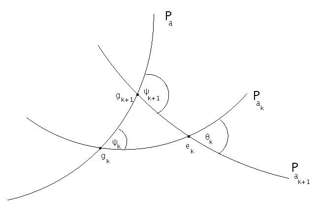
Figure 1. $\psi_{k}+\theta_{k}\leq\psi_{k+1}$

$\Box$

11.2. Facts from hyperbolic trigonometry

The following elementary facts from hyperbolic geometry, which were established in [9], will be used in the proof of Lemma 6.1.

Lemma 11.2.

([9, Lemma 3.1]) Suppose that $T$ is a hyperbolic triangle with a side of length $C$ and opposite angle equal to $\gamma$. Then the triangle has perimeter at most

$$C+2\sinh^{-1}\left(\frac{\sinh(C/2)}{\sin(\gamma/2)}\right)$$

and this maximal perimeter is realized uniquely by an isosceles triangle.

Lemma 11.3.

([9, Lemma 3.2]) Let $P_{0}$, $P_{1}$ and $P_{2}$ be planes in $\mathbb{H}^{3}$ such that $\partial P_{0}$ and $\partial P_{1}$ are tangent in $\hat{\mathbb{C}}$ and $\partial P_{1}$ and $\partial P_{2}$ are also tangent in $\hat{\mathbb{C}}$. If $L\leq 2\sinh^{-1}(1)$ and $\beta:[0,1]\to\mathbb{H}^{3}$ is a curve of length at most $L$ which intersects all three planes, then $P_{0}$ and $P_{2}$ intersect with interior dihedral angle $\theta$, where

$$\theta\geq 2\cos^{-1}\left(\sinh(L/2)\right).$$

In the proof of Lemma 6.6 we will need the following extension of Lemma 11.3 which bounds the length of closed curves intersecting all three sides of a triangle.

Lemma 11.4.

Let $P_{0}$, $P_{1}$ and $P_{2}$ be planes in $\mathbb{H}^{3}$ such that $\partial P_{0}$ and $\partial P_{1}$ are tangent in $\hat{\mathbb{C}}$ and $\partial P_{1}$ and $\partial P_{2}$ are also tangent in $\hat{\mathbb{C}}$. If $P_{0}$ and $P_{2}$ intersect at an interior angle of $\theta$ and $\beta:[0,1]\to\mathbb{H}^{3}$ is a closed curve which intersects all three planes, then $l_{h}(\beta)\geq R(\theta)$, where

$$R(\theta)=\left\{\begin{array}[]{ll}2\sinh^{-1}\left(\frac{1}{\tan(\theta/2)}\right)&\theta>\pi/2\\ 2\sinh^{-1}\left(\frac{\sin(\theta)}{\tan(\theta/2)}\right)&\theta\leq\pi/2\end{array}\right.$$

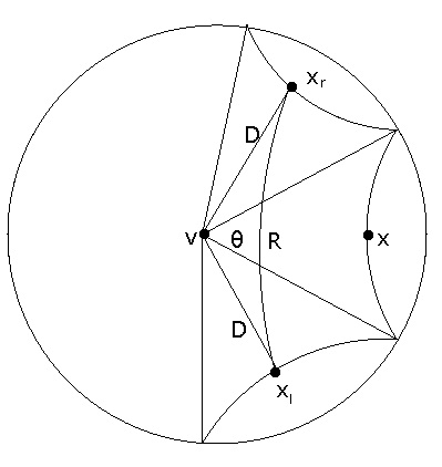
Figure 2. Triangle $T_{\theta}$

Proof.

Let $P$ be the plane which intersects $P_{0}$, $P_{1}$ and $P_{2}$ orthogonally and let $T$ be the triangle they bound in $P$. If $\beta^{\prime}$ is the projection of $\beta$ onto $P$, then $l_{h}(\beta^{\prime})\leq l_{h}(\beta)$ and $\beta^{\prime}$ intersects all three sides of $T$. Therefore, it suffices to bound the length of a curve in $P$ which intersects all three sides of $T$. Since $T$ is convex it suffices to consider curves which lie in $T$.

Let $v$ be the non-ideal vertex of $T$ and let $D$ be length of the perpendicular $\tau$ which joins a point $x$ in the opposite side of $T$ to $v$. Then, by hyperbolic trigonometry, e.g. [2, Theorem 7.11.2],

$$\sinh(D)=\frac{1}{\tan(\theta/2)}.$$

In $\mathbb{H}^{2}$ we take two copies $T_{l}$ and $T_{r}$ of $T$ and glue $T_{l}$ to left edge of $T$ containing $v$ and $T_{r}$ to the right edge containing $v$. We label the points in the copies corresponding to $x$ by $x_{l}$ and $x_{r}$. We can join $x_{l}$ and $x_{r}$ by edges of length $D$ to $v$ which subtend an angle $2\theta$ at $v$ in the union of the three triangles (see figure 2). If $\theta<\pi/2$, we join the points $x_{l}$ and $x_{r}$ by a geodesic $g$ in the union of the three copies and let $R=d(x_{l},x_{r})$. Then we have an isoceles triangle with vertices $x_{l}$ , $x_{r}$, and $v$ and two sides of length $D$ which make an angle $2\theta$. We may decompose this triangle into two right angled triangles with hypotenuse of length $D$ and again apply [2, Theorem 7.11.2] to show that

$$\sinh(D)=\frac{\sinh(l_{h}(g)/2)}{\sin(\theta)}.$$

If $\theta\geq{\pi\over 2}$, then we join $x_{l}$ to $x_{r}$ by a path $g$ of length $2D$ made from copies of $\tau$ in $T_{l}$ and $T_{r}$.

In either case, $g$ projects to a closed curve in $T$ meeting all three sides. To complete the proof, we must show that $g$ projects to the minimal length such curve. If $g^{\prime}$ is the minimal curve, then we may unfold it to a geodesic joining a point $x_{l}^{\prime}$ to the side of $T_{l}$ containing $x_{l}$ to a point $x_{r}^{\prime}$ in the side of $T_{r}$ containing $x_{r}$. Moreover, if we join $x_{l}^{\prime}$ and $x_{r}^{\prime}$ to $v$ by geodesics, the two geodesics each have length at least $D$ and make an angle of $2\theta$. It follows that the length of $g^{\prime}$ is at least as great as that of $g$, with equality if and only if $g=g^{\prime}$. ∎

11.3. Proof of Lemma 6.1

We are now prepared to prove Lemma 6.1, whose statement we recall below:

Lemma 6.1 If  $\Omega$ is the complement of a finite collection $X$ of points in $\hat{\mathbb{C}}$ and $\alpha:[0,1]\rightarrow{\rm Dome}(\Omega)$ is a geodesic path with $l_{h}(\alpha)\leq G({\rm inj}_{{\rm Dome}(\Omega)}(\alpha(s))),$ for some $s\in[0,1]$, then

$$i(\alpha)\leq 2\pi.$$

Proof: Our assumptions imply that there exists $s_{0}\in[0,1]$ such that ${\rm inj}_{{\rm Dome}(\Omega)}(\alpha(s_{0}))\leq F(l_{h}(\alpha))$ (since $G=F^{-1}$). We may assume that $l_{h}(\alpha[0,s_{0}])\leq l_{h}(\alpha)/2$. (If this is not the case we simply consider $\bar{\alpha}:[0,1]\to{\rm Dome}(\Omega)$ given by $\bar{\alpha}(s)=\alpha(1-s)$ and notice that $i(\alpha)=i(\bar{\alpha})$.)

We first handle the case where ${\rm Dome}(\Omega)$ is contained in a plane. In this case, if $i(\alpha)>2\pi$, then there exists a subarc $\alpha_{1}$ containing $\alpha(s_{0})$ with $i(\alpha_{1})=2\pi$. Recall that ${\rm Dome}(\Omega)$ is the double of $CH(X)$ in this case. Both endpoints of $\alpha_{1}$ must lie in the same “copy” of $CH(X)$. One may then join the endpoints of $\alpha_{1}$ by a geodesic arc $\beta$ in this copy, so that $\delta=\alpha_{1}\cup\beta$ is homotopically non-trivial in ${\rm Dome}(\Omega)$ and $l(\delta)<2l(\alpha)$. It follows that

$${\rm inj}_{{\rm Dome}(\Omega)}(\alpha(s_{0}))<l_{h}(\alpha)<F(l_{h}(\alpha))$$

which is a contradiction.

We now move on to the general case. Let $\{P_{t}\ |\ 0\leq t\leq i(\alpha)\}$ be the full family of support planes to $\alpha$. There are three cases.

Case 1: If $H_{t}\cap H_{0}\neq\emptyset$ for all $t$, then Lemma 11.1 implies that

$$i(\alpha)\leq\pi.$$

If we are not in case 1, let $P_{t_{1}}$ be the first support plane with $H_{t_{1}}\cap H_{0}=\emptyset$

Case 2: If $H_{t}\cap H_{t_{1}}$ for all $t\geq t_{1}$, then by applying Lemma 11.1 to the two families $\{P_{t}\ |\ 0\leq t<t_{1}\}$ and $\{P_{t}\ |\ t_{1}\leq t\leq i(\alpha)\}$, we have

$$i(\alpha)\leq\pi+\pi=2\pi.$$

Case 3: If we are not in case (1) or (2), we let $P_{t_{2}}$ be the first support plane such that $H_{t_{2}}\cap H_{t_{1}}=\emptyset$. Consider the configuration of three planes $P_{0}$, $P_{t_{1}}$, and $P_{t_{2}}$. Let $\alpha_{1}=\alpha|_{[0,s_{1}]}$ be the subarc of $\alpha$ of minimum length having $\{P_{t}\ |\ 0\leq t\leq t_{2}\}$ as a family of support planes. Let $x$ and $y$ be the endpoints of $\alpha_{1}$. Lemma 11.3 implies that $P_{0}$ and $P_{t_{2}}$ intersect and have dihedral angle $\theta$ satisfying

$$\theta\geq 2\cos^{-1}(\sinh(l_{h}(\alpha_{1})/2)).$$

We join $x$ to $y$ by a shortest path $\beta$ on $P_{0}\cup P_{t_{2}}$ which intersects $P_{0}\cap P_{t_{2}}$ at a point $z\in P_{0}\cap P_{t_{2}}$. We take the triangle $T$ with vertices $x$, $y$, and $z$. Then the interior angle $\theta_{z}$ of $T$ at $z$ satisfies $\theta_{z}\geq\theta$. Since $x$ and $y$ lie in $\alpha_{1}$, $d(x,y)\leq l_{h}(\alpha_{1})$. Then, by Lemma 11.2,

$$d(x,z)+d(z,y)\leq 2\sinh^{-1}\left(\frac{\sinh(d(x,y)/2)}{\sin(\theta_{z}/2)}\right)\leq 2\sinh^{-1}\left(\frac{\sinh(l_{h}(\alpha_{1})/2)}{\sin(\theta/2)}\right).$$

Substituting the bound for $\theta$ we get

$$d(x,z)+d(z,y)\leq 2\sinh^{-1}\left(\frac{\sinh(l_{h}(\alpha_{1})/2)}{\sqrt{1-\sinh^{2}(l_{h}(\alpha_{1})/2)}}\right).$$

If $\delta=\alpha_{1}\cup\beta$, then

$$l_{h}(\delta)\leq l_{h}(\alpha_{1})+2\sinh^{-1}\left(\frac{\sinh\left({l_{h}(\alpha_{1})\over 2}\right)}{\sqrt{1-\sinh^{2}\left({l_{h}(\alpha_{1})\over 2}\right)}}\right)=2F(l_{h}(\alpha_{1})).$$

We next show that $r(\delta)$ is homotopically non-trivial on ${\rm Dome}(\Omega)$. Since the restriction of $r$ to $\mathbb{H}^{3}-{\rm int}(CH(X)))$ is a homotopy equivalence onto ${\rm Dome}(\Omega)$, it suffices to show that $\delta$ is homotopically non-trivial in $\mathbb{H}^{3}-{\rm int}(CH(X)).$ Let $b=\alpha(s_{1})$ be the first point on $\alpha$ which has support plane $P_{t_{1}}$. Then $b$ lies on an edge $e$ of ${\rm Dome}(\Omega)$ which is contained in $P_{t_{1}}$. Let $Q_{b}$ be the plane through $b$ which is perpendicular to $P_{t_{1}}$ and let $R_{b}$ be the intersection of $Q_{b}$ with the closed half-space bounded by $P_{t_{1}}$ which is disjoint from ${\rm int}(CH(X))$. Lemma 11.1 implies that $\alpha_{1}$ intersects $b$ exactly once at $\alpha(s_{1})$ and the intersection is transverse. By construction, $\beta$ cannot intersect $R_{b}$ and $\alpha_{1}$ cannot intersect $R_{b}-b$. Therefore, $\delta$ intersects $R_{b}$ exactly once and does so transversely. Since $R_{b}$ is a properly embedded half-plane in $\mathbb{H}^{3}-{\rm int}(CH(X))$, we see that $\delta$ is homotopically non-trivial in $\mathbb{H}^{3}-{\rm int}(CH(X))$ as desired.

Since $r$ is 1-Lipschitz on $\mathbb{H}^{3}$,

$$l_{h}(r(\delta))\leq l_{h}(\delta)\leq 2F(l_{h}(\alpha_{1}))<2F(l_{h}(\alpha)).$$

In particular, since $r(\delta)$ is homotopically non-trivial and passes through $\alpha(0)$, we see that

$${\rm inj}_{{\rm Dome}(\Omega)}(x)\leq F(l_{h}(\alpha))$$

for all $x\in\alpha_{1}$. If $\alpha(s_{1})\in\alpha_{1}$, i.e. if $s_{0}\leq s_{1}$, then we have achieved a contradiction and we are done. If $\alpha(s_{0})$ does not lie in $\alpha_{1}$, then let $\alpha_{2}=\alpha|_{[s_{1},s_{0}]}$. Then $\gamma=\bar{\alpha}_{2}*\bar{r}(\beta)*\alpha_{1}*\alpha_{2}$ is a homotopically non-trivial loop through $\alpha(s_{0})$ such that

$$l_{h}(\gamma)=2l_{h}(\alpha_{2})+l_{h}(r(\delta))<l_{h}(\alpha)+2F(l_{h}(\alpha_{1})).$$

Since

$$l_{h}(\alpha)+2F(l_{h}(\alpha_{1}))<l_{h}(\alpha)+2F(l_{h}(\alpha)/2)<2F(l_{h}(\alpha))$$

we have again achieved a contradiction. $\Box$

11.4. Proof of Lemma 6.6

We now establish Lemma 6.6 which bounds intersection number for short simple closed geodesics.

Lemma 6.6 Suppose that $\Omega$ is the complement of finite collection $X$ of points in $\hat{\mathbb{C}}$. If $\gamma$ is a simple closed geodesic of length less than $2\sinh^{-1}(1)$, then

$$2\pi\leq i(\gamma)\leq 2\pi+2\tan^{-1}(\sinh(l_{h}(\gamma)/2))\leq\frac{5\pi}{2}$$

Proof.

We first note that if ${\rm Dome}(\Omega)$ lies in a plane and $\gamma$ is a simple closed geodesic on ${\rm Dome}(\Omega)$, then $\gamma$ is the double of a simple geodesic arc in $CH(X)$, so $i(\gamma)=2\pi$.

For the remainder of the proof, we assume that $CH(X)$ does not lie in a plane. We choose a parameterization $\alpha:[0,1]\rightarrow{\rm Dome}(\Omega)$ of $\gamma$ which is an embedding on $(0,1)$ and such that $\alpha(0)=\alpha(1)$ does not lie on an edge of ${\rm Dome}(\Omega)$. Recall that Lemma 6.4 implies that $i(\gamma)\geq 2\pi$.

Let $\{P_{t}\ |\ 0\leq t\leq i(\alpha)\}$ be the full family of support planes to $\alpha$. If we proceed as in the proof of Lemma 6.1, we must be in case (3). Therefore, we obtain support planes $P_{0}$, $P_{t_{1}}$ and $P_{t_{2}}$, such that $\partial P_{0}$ and $\partial P_{t_{1}}$ are tangent on $\hat{\mathbb{C}}$, as are $P_{t_{1}}$ and $P_{t_{2}}$, and a subarc $\alpha_{1}$ of $\alpha$ which begins at $\alpha(0)\in P_{0}$, ends at $\alpha(s_{1})\in P_{t_{2}}$ and intersects $P_{t_{1}}$. Lemma 11.3 implies that $P_{0}$ and $P_{t_{2}}$ intersect. Lemma 11.4 implies that if $\theta$ is the angle of intersection of $P_{0}$ and $P_{t_{2}}$, then $\theta\geq R^{-1}(l_{h}(\gamma)).$ As $R$ is decreasing and $R(\pi/2)=2\sinh^{-1}(1)\geq l_{h}(\gamma)$ we see that $\theta\geq\pi/2$.

Therefore,

$$\theta\geq R^{-1}(l_{h}(\gamma))=2\tan^{-1}\left(\frac{1}{\sinh\left(\frac{l_{h}(\gamma)}{2}\right)}\right)$$

Let $\phi=\pi-\theta\leq\pi/2$ be the exterior dihedral angle between $P_{0}$ and $P_{t_{2}}$. Then,

$$\phi\leq 2\tan^{-1}(\sinh(l_{h}(\gamma)/2)).$$

Let $\beta_{0}$ be the shortest path on $P_{0}\cup P_{t_{2}}$ joining $\alpha(0)$ to $\alpha(s_{1})$ and let $z_{0}$ be the point of intersection of $\beta_{0}$ with $P_{0}\cap P_{t_{2}}$. Since

$$d_{h}(\alpha(0),\alpha(s_{1}))\leq l_{h}(\gamma)/2,$$

Lemma 11.2 implies that

$$l_{h}(\beta_{0})\leq 2\sinh^{-1}\left(\frac{\sinh(d_{h}(\alpha(0),\alpha(s_{1}))/2)}{\sin(\theta/2)}\right),$$

so

$$\sinh(l_{h}(\beta_{0})/2)\leq\frac{\sinh(l_{h}(\gamma)/4)}{\sin(\theta/2)}.$$

Since $\theta\geq{\pi\over 2}$ and $l_{h}(\gamma)<2\sinh^{-1}(1)$, we see that

$$\sinh(l_{h}(\beta_{0})/2)\leq\frac{\sinh(\frac{\sinh^{-1}(1)}{2})}{\sin(\frac{\pi}{4})}\approx.6436<1.$$

It follows that $l_{h}(\beta_{0})/2<\sinh^{-1}(1)$.

We let $\delta_{0}=\alpha_{1}\cup\beta_{0}$. We may argue, exactly as in the proof of Lemma 6.6, that $r(\delta_{0})$ is homotopically non-trivial on ${\rm Dome}(\Omega)$. Since $\alpha_{1}\subset\gamma$, $l_{h}(\beta_{0})/2<\sinh^{-1}(1)$ and $N(\gamma)$ has width $w(\gamma)>\sinh^{-1}(1)$, we see that $r(\delta_{0})$ is contained in $N(\gamma)$, so is homotopic to a non-trivial power of $\gamma$.

We now describe a process to replace $\beta_{0}$ by a path $\beta_{n}$ on ${\rm Dome}(\Omega)$ such that $i(\beta_{n})\leq\phi$ and $\beta_{n}$ is homotopic to $r(\beta_{0})$. Once we have done so, we can form $\delta_{n}=\alpha_{1}\cup\beta_{n}$ and observe that

$$i(\delta_{n})\leq i(\alpha_{1})+\phi\leq 2\pi+\phi\leq 2\pi+2\tan^{-1}(\sinh(l_{h}(\alpha_{1})/2))\leq{5\pi\over 2}.$$

Our result follows, since $\delta_{n}$ is homotopic to a non-trivial power of $\gamma$ and a geodesic minimizes intersection number in its homotopy class.

We label $Q_{0}=P_{t_{2}}$ and let $P_{0}\cap Q_{0}=h_{0}$. If $h_{0}$ is an edge then $P_{0}$ and $Q_{0}$ are adjacent and $\beta_{0}$ is on ${\rm Dome}(\Omega)$ and we are done.

Otherwise $\beta_{0}$ intersects an edge on $Q_{0}$ labelled $e_{0}$, such that $h_{0}$ and $e_{0}$ are disjoint. We choose $e_{0}$ to be the last edge on $Q_{0}$ that $\alpha$ intersects. Let $y_{0}$ be the first point of intersection of $\beta_{0}$ and $e_{0}$. Let $F_{1}$ be the face of ${\rm Dome}(\Omega)$ which abuts $e_{0}$ and does not contain a subarc of $\beta_{0}$. Let $Q_{1}$ be the support plane containing $F_{1}$.

Define $h_{1}=P_{0}\cap Q_{1}$. Since $h_{0}$ and $h_{1}$ are both contained in support planes to $e_{0}$, they are disjoint. Since $\alpha(0)\in{\rm Dome}(\Omega)$, $h_{0}$ must separate $h_{1}$ from $\alpha(0)$ in $P_{0}$. Therefore, $\beta_{0}$ intersects $h_{1}$ at a point $z_{1}$ between $z_{0}$ and $\alpha(0)$. We construct $\beta_{1}$ by replacing the subarc of $\beta_{0}$ joining $y_{0}$ to $z_{1}$ by the geodesic arc in $F_{1}$ joining $y_{0}$ to $z_{1}$. Notice that $r(\beta_{1})$ is homotopic to $r(\beta_{0})$ in ${\rm Dome}(\Omega)$. If we let $\theta_{1}$ be the exterior dihedral angle between $Q_{0}$ and $Q_{1}$ and let $\phi_{1}$ be the exterior dihedral angle between $Q_{1}$ and $P_{0}$, then

$$\theta_{1}+\phi_{1}\leq\phi.$$

If $h_{1}$ is an edge, then $\beta_{1}$ lies on ${\rm Dome}(\Omega)$ and we are done since

$$i(\beta_{1})=\theta_{1}+\phi_{1}\leq\phi.$$

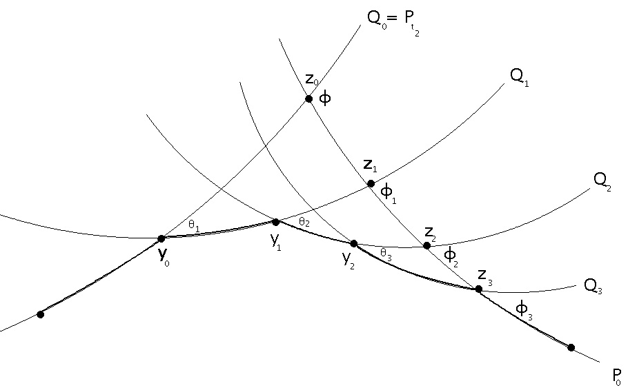
Figure 3. $\beta_{n}=\beta_{3}$

If $h_{1}$ is not an edge, we define $\beta_{n}$ by an iterative procedure. Assume $Q_{k}$ are defined as above, for $k=0,\ldots,m$, such that $h_{m}=Q_{m}\cap P_{0}$ is not an edge. Define $\theta_{k}$ to be the exterior dihedral angle between $Q_{k-1}$ and $Q_{k}$ and $\phi_{k}$ to be the exterior dihedral angle between $Q_{k}$ and $P_{0}$. We assume, by induction, that

$$\sum_{k=1}^{m}\theta_{k}+\phi_{m}\leq\phi.$$

Let $h_{m}$ be the last edge on $Q_{m}$ which $\beta_{m}$ intersects, and let $y_{m}$ be the first point of intersection of $\beta_{m}$ and $h_{m}$. Let $F_{m+1}$ be the face adjacent to $e_{m}$ which does not agree with $F_{m}$ and let $Q_{m+1}$ be the support plane it is contained in. As before, if we let $h_{m+1}=Q_{m+1}\cap P_{0}$, then $h_{m+1}$ separates $h_{m}$ from $\alpha(0)$. Therefore, $\beta_{m}$ intersects $h_{m+1}$ in a point $z_{m+1}$. We construct $\beta_{m+1}$ by replacing the piecewise geodesic subarc of $\beta_{m}$ connecting $y_{m+1}$ to $z_{m+1}$ by the geodesic arc in $F_{m+1}$ joining $y_{m+1}$ to $z_{m+1}$. Again, notice that $r(\beta_{m+1})$ is homotopic to $r(\beta_{m})$. Furthermore,

$$\theta_{m+1}+\phi_{m+1}\leq\phi_{m}.$$

Therefore,

$$\sum_{k=1}^{m+1}\theta_{k}+\phi_{m+1}=\sum_{k=1}^{n}\theta_{k}+(\theta_{m+1}+\phi_{m+1})\leq\sum_{k=1}^{m}\theta_{m}+\phi_{m}\leq\phi.$$

Notice that the support planes $\{Q_{k}\}$ in this procedure have disjoint intersection with $P_{0}$ and each contain a face $F_{k}$. Therefore, as there are only a finite number of faces, the process terminates and some $h_{n}$ is an edge of ${\rm Dome}(\Omega)$. Then, $\beta_{n}$ lies on ${\rm Dome}(\Omega)$ and our argument is complete. ∎

References

- [1]
- [2] A. Beardon,The Geometry of Discrete Groups, Springer-Verlag, 1995
- [3] A. Beardon and C. Pommerenke “The Poincaré metric of plane domains,” J. London Math. Soc., 18, (1978), 475-83.
- [4] C.J. Bishop, “Divergence groups have the Bowen property,” Annals of Math. 154(2001), 205–217.
- [5] C.J. Bishop, “Quasiconformal Lipschitz maps, Sullivan’s convex hull theorem and Brennan’s conjecture,” Ark. Mat. 40(2002), 1–26.
- [6] C.J. Bishop, “An explicit constant for Sullivan’s convex hull theorem,” in In the tradition of Ahlfors and Bers III, Contemp. Math. 355(2007), Amer. Math. Soc., 41–69.
- [7] B.H. Bowditch, “Some results on the geometry of convex hulls in manifolds of pinched negative curvature,” Comm. Math. Helv. 69(1994), 49–81.
- [8] M. Bridgeman, “Average bending of convex pleated planes in hyperbolic three-space,” Invent. Math. 132(1998), 381–391.
- [9] M. Bridgeman and R.D. Canary, “From the boundary of the convex core to the conformal boundary,” Geometrica Dedicata 96(2003), 211–240.
- [10] X. Buff, J. Fehrenbach, P. Lochak, L. Schneps, and P. Vogel, Moduli Spaces of Curves, Mapping Class Groups and Field Theory, American Mathematical Society, 2003.
- [11] P. Buser, Geometry and Spectra of Compact Hyperbolic Surfaces, Birkhäuser, 1992.
- [12] R.D. Canary, “The Poincaré metric and a conformal version of a theorem of Thurston,” Duke Math. J. 64(1991), 349–359.
- [13] R.D. Canary, “The conformal boundary and the boundary of the convex core,” Duke Math. J. 106(2001), 193–207.
- [14] A. Douady and C. Earle, “Conformally natural extensions of homeomorphisms of the circle,” Acta. Math. 157(1986), 23–48.
- [15] D.B.A. Epstein and A. Marden, “Convex hulls in hyperbolic space, a theorem of Sullivan, and measured pleated surfaces,” in Analytical and Geometrical Aspects of Hyperbolic Space, Cambridge University Press, 1987, 113–253.
- [16] D.B.A. Epstein, A. Marden and V. Markovic, “Quasiconformal homeomorphisms and the convex hull boundary,” Ann. of. Math. 159(2004), 305–336.
- [17] D.B.A. Epstein, A. Marden and V. Markovic, “Complex earthquakes and deformations of the unit disk,” J. Diff. Geom 73(2006), 119–166.
- [18] D.B.A. Epstein and V. Markovic, “The logarithmic spiral: a counterexample to the conjecture,” Ann. of Math. 161(2005), 925–957.
- [19] A. Fletcher and V. Markovic, Quasiconformal maps and Teichmüller theory, Oxford University Press, 2007.
- [20] F.W. Gehring and B. Palka, “Quasiconformally homogeneous domains,” J. Anal. Math. 30 (1976), 172–199.
- [21] D. Herron, W. Ma and D. Minda,“Estimates for conformal metric ratios,” Computational Methods and Function Theory. 5 (2), (2005), 323–345.
- [22] M. Kapovich “Hyperbolic Manifolds and Discrete Groups”, Progress in Mathematics Series, Birhaüser, (2001).
- [23] R. Kulkarni and U. Pinkall, “A canonical metric for Möbius structures and its applications,” Math. Z. 216(1994), 89–129.
- [24] M.Lehtinen, “The dilatation of Beurling-Ahlfors extensions of quasisymmetric functions,” Ann. Acad. Sci. Fenn. 8(1983), 187–191.
- [25] A. Marden and V. Markovic, “Characterizations of plane regions that support quasiconformal mappings to their domes,” Bull. L.M.S. 39(2007), 962–972.
- [26] C.T. McMullen, “Complex earthquakes and Teichmüller theory,” J. Amer. Math. Soc. 11(1998), 283–320.
- [27] C. Pommerenke, “On uniformly perfect sets and Fuchsian groups,” Analysis 4(1984) 299–321.
- [28] D.P. Sullivan, “Travaux de Thurston sur les groupes quasi-fuchsiens et les variétés hyperboliques de dimension fibrées sur ,” in Bourbaki Seminar, Vol. 1979/1980, Lecture Notes in Math. 842(1981), 196–214.
- [29] H, Tanigawa, “Grafting, harmonic maps and projective structures,” J. Diff. Geom. 47(1997), 399–419.
- [30] W.P. Thurston, The Geometry and Topology of -Manifolds, Lecture Notes, Princeton University, 1979.
- [31]