Solitary Waves in Massive Nonlinear $\mathbb{S}^{N}$-Sigma Models

Solitary Waves in Massive
Nonlinear $\boldsymbol{\mathbb{S}^{N}}$-Sigma Models

Alberto ALONSO IZQUIERDO ^†, Miguel Ángel GONZÁLEZ LEÓN ^†
and Marina DE LA TORRE MAYADO ^‡

A. Alonso Izquierdo, Ḿ.A. González León and M. de la Torre Mayado

^† Departamento de Matemática Aplicada, Universidad de Salamanca, Spain alonsoiz@usal.es, magleon@usal.es http://campus.usal.es/~mpg/

^‡ Departamento de Física Fundamental, Universidad de Salamanca, Spain marina@usal.es

Received December 07, 2009; Published online February 09, 2010

The solitary waves of massive $(1+1)$-dimensional nonlinear ${\mathbb{S}}^{N}$-sigma models are unveiled. It is shown that the solitary waves in these systems are in one-to-one correspondence with the separatrix trajectories in the repulsive $N$-dimensional Neumann mechanical problem. There are topological (heteroclinic trajectories) and non-topological (homoclinic trajectories) kinks. The stability of some embedded sine-Gordon kinks is discussed by means of the direct estimation of the spectra of the second-order fluctuation operators around them, whereas the instability of other topological and non-topological kinks is established applying the Morse index theorem.

solitary waves; nonlinear sigma models

35Q51; 81T99

1 Introduction

The existence and the study of solitary waves in $(1+1)$-dimensional relativistic field theories is of the greatest interest in several scientific domains. We specifically mention high energy physics, applied mathematics, condensed matter physics, cosmology, fluid dynamics, semiconductor physics, etcetera. Solitary waves have been discovered recently in massive nonlinear sigma models with quite striking properties, see e.g. [2, 3, 4] and references quoted therein. The nonlinear ${\mathbb{S}}^{N}$-sigma models are important in describing the low energy pion dynamics in nuclear physics [5] and/or featuring the long wavelength behavior of ${\mathbb{O}}(N+1)$-spin chains in ferromagnetic materials [6].

In this work, we present a mathematically detailed analysis of the solitary wave manifold arising in a massive ${\mathbb{S}}^{N}$-sigma model that extends and generalize previous work performed in [2] and [3] on the $N=2$ case. In these papers the masses of the $N=2$ meson branches are chosen to be different by breaking the ${\mathbb{O}}(N)$ degeneracy of the ground state to a ${\mathbb{Z}}_{2}$ sub-group. Remarkably, we recognized in [2] and [3] that the static field equations of this non-isotropic massive nonlinear ${\mathbb{S}}^{2}$-sigma model are the massive version of the static Landau–Lifshitz equations governing the high spin and long wavelength limit of 1D ferromagnetic materials. This perspective allows to interpret the topological kinks of the model as Bloch and Ising walls that form interfaces between ferromagnetic domains, see [7, 8, 9].

We shall proceed into a two-step mathematical analysis: First, we shall identify the collection of $N$ sine-Gordon models embedded in our nonlinear ${\mathbb{S}}^{N}$-sigma models. The sine-Gordon kinks (and the sine-Gordon multi-solitons) are automatically solitary waves (and multi-solitons) in the nonlinear sigma model. Second, we shall identify the static field-equations as the Newton equations of the repulsive Neumann problem in the ${\mathbb{S}}^{N}$-sphere. The mechanical analogy in the search for solitary waves in $(1+1)$-dimensional relativistic field theories, [10], is the re-reading of the static field equations as the motion equations of a mechanical system where the field theoretical spatial coordinate is re-interpreted as the “mechanical time” and the potential energy density is minus the “mechanical potential”. This strategy is particularly efficient in field theories with a single scalar field because in such a case the mechanical analogue problem has only one degree of freedom and one can always integrate the motion equations.

The mechanical analogue system of field theoretical models with $N$ scalar fields has $N$ degrees of freedom and the system of $N$ motion ODE’s is rarely integrable. One may analytically find the solitary waves in field theories such that their associated mechanical system is completely integrable. Many solitary waves have been found in two scalar field models related to the Garnier integrable system of two degrees of freedom and other Liouville models, see [11]. The extremely rich structure of such varieties of kinks has been exhaustively described in [12]. The procedure can be also extended to systems with $N=3$ (and higher) degrees of freedom that are Hamilton–Jacobi separable using Jacobi elliptic coordinates, see [13]. The mechanical analogue system of the non-isotropic massive nonlinear ${\mathbb{S}}^{N}$-system is the Neumann system, a particle constrained to move in a ${\mathbb{S}}^{N}$-sphere subjected to elastic repulsive non-isotropic forces from the origin. It happens that the Neumann system [14, 15, 16] is not only Arnold–Liouville completely integrable – there are $N$ constants of motion in involution – but Hamilton–Jacobi separable using sphero-conical coordinates. Because the elastic forces are repulsive the North and South poles are unstable equilibrium points where heteroclinic and homoclinic trajectories start and end providing the solitary waves of the nonlinear sigma model.

The analysis of the stability of solitary waves against small fluctuations is tantamount to the study of the linearized wave equations around a particular traveling wave. We shall distinguish between stable and unstable sine-Gordon kinks by means of the determination of the spectra of small fluctuations around these embedded kinks. The instability of any other (not sine-Gordon) solitary wave in the nonlinear ${\mathbb{S}}^{3}$-sigma model will be shown by computing the Jacobi fields between conjugate points along the trajectory and using the Morse index theorem within the framework explained in [17].

The structure of the article is as follows: In Section 2 we present the fundamental aspects of the model. Section 3 is devoted to the study of the set of sine-Gordon models that are embedded in the nonlinear ${\mathbb{S}}^{N}$-sigma model. In Section 4, using sphero-conical coordinates, we show the separability of the Hamilton–Jacobi equation that reduces to $N$ uncoupled ODE. The Hamilton characteristic function is subsequently found as the sum of $N$ functions, each one depending only on one coordinate, and the separation constants are chosen in such a way that the mechanical energy is zero. Then, the motion equations are solved by quadratures. The properties and structure of the explicit analytic solutions are discussed respectively in Sections 5 and 6 for the $N=2$ and $N=3$ models. Finally, in Section 7 the stability analysis of the solitary wave solutions is performed.

2 The massive nonlinear $\boldsymbol{{\mathbb{S}}^{N}}$-sigma model

Let us consider $N+1$ real scalar fields arranged in a vector-field:

$$\vec{\Phi}\big{(}y^{0},y^{1}\big{)}\equiv\big{(}\phi_{1}\big{(}y^{0},y^{1}\big{)},\dots,\phi_{N+1}\big{(}y^{0},y^{1}\big{)}\big{)},$$

where $\big{(}y^{0},y^{1}\big{)}$ stand for the standard coordinates in the Minkowski space ${\mathbb{R}}^{1,1}$, and the fields are constrained to be in the ${\mathbb{S}}^{N}$-sphere, i.e.

$$\vec{\Phi}\in{\rm Maps}\left({\mathbb{R}}^{1,1},{\mathbb{S}}^{N}\right),\qquad\vec{\Phi}\cdot\vec{\Phi}=\phi_{1}^{2}+\dots+\phi_{N+1}^{2}=R^{2}.$$ (2.1)

The dynamics of the model is governed by the action functional:

$$S[\vec{\Phi}]=\int dy^{0}dy^{1}\,{\cal L}\big{(}\partial_{\mu}\vec{\Phi},\vec{\Phi}\big{)}=\int dy^{0}dy^{1}\left\{\frac{1}{2}\partial_{\mu}\vec{\Phi}\cdot\partial^{\mu}\vec{\Phi}-V(\vec{\Phi})\right\},$$

where $V(\vec{\Phi})$ is the quadratic polynomial function in the fields:

$$V(\vec{\Phi})=\tfrac{1}{2}\left(\alpha_{1}^{2}\phi_{1}^{2}+\alpha_{2}^{2}\phi_{2}^{2}+\dots+\alpha_{N+1}^{2}\phi_{N+1}^{2}-\alpha_{N+1}^{2}R^{2}\right).$$ (2.2)

We follow standard Minkowski space conventions: $y^{\mu}y_{\mu}=g^{\mu\nu}y_{\mu}y_{\nu}$, $g^{\mu\nu}={\rm diag}(1,-1)$, $\partial_{\mu}\partial^{\mu}=g^{\mu\nu}\partial_{\mu}\partial_{\nu}=\partial_{0}^{2}-\partial_{1}^{2}$. Working in the natural system of units, $\hbar=c=1$, the dimensions of the fields and parameters are: $[\phi_{a}]=[R]=1$, $[\alpha_{a}]=M$, $a=1,\dots,N+1$.

The field equations of the system are:

$$\partial_{\mu}\left(\frac{\partial{\cal L}}{\partial(\partial_{\mu}\phi_{a})}\right)-\frac{\partial{\cal L}}{\partial\phi_{a}}=0\ \Rightarrow\ \partial_{0}^{2}\phi_{a}-\partial_{1}^{2}\phi_{a}=-\alpha_{a}^{2}\phi_{a}+\lambda\phi_{a},\qquad a=1,\dots,N+1,$$ (2.3)

$\lambda$ being the Lagrange multiplier associated to the constraint (2.1). $\lambda$ can be expressed in terms of the fields and their first derivatives:

$$\lambda=\frac{1}{R^{2}}\left(\sum_{a=1}^{N+1}\alpha_{a}^{2}\phi_{a}^{2}-\partial_{0}\vec{\Phi}\cdot\partial_{0}\vec{\Phi}+\partial_{1}\vec{\Phi}\cdot\partial_{1}\vec{\Phi}\right)$$

by successive differentiations of the constraint equation (2.1). There exists $N+1$ static and homogeneous solutions of (2.3) on ${\mathbb{S}}^{N}$:

$$\phi_{a}=\pm R,\qquad\phi_{b}=0,\quad\forall\,b\neq a,\qquad\lambda=\alpha_{a}^{2},\qquad a=1,\dots,N+1.$$ (2.4)

We shall address the maximally anisotropic case: $\alpha_{a}\neq\alpha_{b}$, $\forall\,a\neq b$, and, without loss of generality, we label the parameters in decreasing order: $\alpha_{1}^{2}>\alpha_{2}^{2}>\cdots>\alpha_{N+1}^{2}\geq 0$, in such a way that $V(\vec{\Phi})$, on the ${\mathbb{S}}^{N}$-sphere (2.1), is semi-definite positive.

According to Rajaraman [10] solitary waves (kinks) are non-singular solutions of the field equations (2.3) of finite energy such that their energy density has a space-time dependence of the form: $\varepsilon(y^{0},y^{1})=\varepsilon(y^{1}-vy^{0})$, where $v$ is some velocity vector. The energy functional is:

$$E[\vec{\Phi}]=\displaystyle\int dy^{1}\left(\frac{1}{2}\partial_{0}\vec{\Phi}\cdot\partial_{0}\vec{\Phi}+\frac{1}{2}\partial_{1}\vec{\Phi}\cdot\partial_{1}\vec{\Phi}+V\big{(}\vec{\Phi}\big{)}\right)=\int dy^{1}\varepsilon\big{(}y^{0},y^{1}\big{)}$$

and the integrand $\varepsilon\big{(}y^{0},y^{1}\big{)}$ is the energy density. Lorentz invariance of the model implies that it suffices to know the $y^{0}$-independent solutions $\vec{\Phi}\big{(}y^{1}\big{)}$ in order to obtain the traveling waves of the model: $\vec{\Phi}\big{(}y^{0},y^{1}\big{)}=\vec{\Phi}\big{(}y^{1}-vy^{0}\big{)}$. For static configurations the energy functional reduces to:

$$E[\vec{\Phi}]=\int dy^{1}\left(\frac{1}{2}\frac{d\vec{\Phi}}{dy^{1}}\cdot\frac{d\vec{\Phi}}{dy^{1}}+V\big{(}\vec{\Phi}\big{)}\right)=\int dy^{1}\varepsilon\big{(}y^{1}\big{)}.$$ (2.5)

and the PDE system (2.3) becomes the following system of $N+1$ ordinary differential equations:

$$\frac{d^{2}\phi_{a}}{d(y^{1})^{2}}=\alpha_{a}^{2}\phi_{a}-\lambda\phi_{a}.$$ (2.6)

The finite energy requirement selects between the static and homogeneous solutions (2.4) only two, the set ${\cal M}$ of zeroes (and absolute minima) of $V(\vec{\Phi})$ on ${\mathbb{S}}^{N}$:

$${\cal M}=\left\{v^{+}=(0,\dots,0,R),\ v^{-}=(0,\dots,0,-R)\right\},$$

i.e. the “North” and the “South” poles of the ${\mathbb{S}}^{N}$-sphere. Moreover, this requirement forces in (2.5) the asymptotic conditions:

$$\lim_{y^{1}\to\pm\infty}\frac{d\vec{\Phi}}{dy^{1}}=0,\qquad\lim_{y^{1}\to\pm\infty}\vec{\Phi}\in{\cal M}.$$ (2.7)

Consequently, the configuration space, the space of finite energy configurations:

$${\cal C}=\left\{{\rm Maps}({\mathbb{R}},{\mathbb{S}}^{n})/E<+\infty\right\},$$

is the union of four disconnected sectors: ${\cal C}={\cal C}_{\rm NN}\bigcup{\cal C}_{\rm SS}\bigcup{\cal C}_{\rm NS}\bigcup{\cal C}_{\rm SN}$, where the different sectors are labeled by the element of ${\cal M}$ reached by each configuration at $y^{1}\to-\infty$ and $y^{1}\to\infty$. ${\cal C}_{\rm NS}$ and ${\cal C}_{\rm SN}$ solitary waves will be termed as topological kinks, whereas non-topological kinks belong to ${\cal C}_{\rm NN}$ or ${\cal C}_{\rm SS}$.

3 Embedded sine-Gordon models

Before of embarking ourselves in the general solution of the ODE system (2.6), we explore Rajaraman’s trial-orbit method [10]. We search for solitary wave solutions living on special meridians of the ${\mathbb{S}}^{N}$-sphere such that the associated trajectories connect the North and South poles, to comply with the asymptotic conditions of finite energy (2.7). In [2] and [3] this strategy was tested in the $N=2$ case. It was easily proved that the nonlinear sigma model reduces to a sine-Gordon model only over the meridians in the intersection of the coordinate planes in ${\mathbb{R}}^{3}$ with the ${\mathbb{S}}^{2}$-sphere, that contain the North and South poles. Consequently, there are sine-Gordon kinks (and multi-solitons) embedded in the nonlinear sigma model living in these meridians. The generalization to any $N$ is immediate: the $N$ meridians $m_{a}$, $a=1,\dots,N$, determined by the intersection of the $\phi_{a}-\phi_{N+1}$ plane with the ${\mathbb{S}}^{N}$-sphere, all of them containing the points N and S,

$$m_{a}\Rightarrow\phi_{b}=0,\quad\forall\,b\neq a,\ \ b=1,\dots,N,\qquad\phi_{a}^{2}+\phi_{N+1}^{2}=R^{2},\quad a=1,\dots,N,$$

are good trial orbits on which the field equations (2.3) reduce to the system of two PDE’s:

$$\partial_{0}^{2}\phi_{a}-\partial_{1}^{2}\phi_{a}=-\alpha_{a}^{2}\phi_{a}+\lambda\phi_{a},$$ (3.1)

$$\partial_{0}^{2}\phi_{N+1}-\partial_{1}^{2}\phi_{N+1}=-\alpha_{N+1}^{2}\phi_{N+1}+\lambda\phi_{N+1}.$$ (3.2)

Use of “polar” coordinates in the $\phi_{a}-\phi_{N+1}$ plane:

$$\phi_{N+1}=R\cos\theta,\qquad\phi_{a}=\pm R\sin\theta,\qquad\theta\in[0,\pi]$$

reveals that the two equations (3.1), (3.2) are tantamount to the sine-Gordon equation in the half-meridians ${\rm sign}(\phi_{a})=\pm 1$:

$$\partial_{0}^{2}\theta-\partial_{1}^{2}\theta=-\tfrac{1}{2}\left(\alpha_{a}^{2}-\alpha_{N+1}^{2}\right)\sin 2\theta.$$ (3.3)

For the sake of simplicity it is convenient to define non dimensional parameters and coordinates in the Minkowski space ${\mathbb{R}}^{1,1}$:

$$\begin{split}&\sigma_{a}^{2}=\frac{\alpha_{a}^{2}-\alpha_{N+1}^{2}}{\alpha_{1}^{2}-\alpha_{N+1}^{2}},\qquad 1=\sigma_{1}^{2}>\sigma_{2}^{2}>\dots>\sigma_{N}^{2}>0=\sigma_{N+1}^{2},\\ &t=\sqrt{\alpha_{1}^{2}-\alpha_{N+1}^{2}}y^{0},\qquad x=\sqrt{\alpha_{1}^{2}-\alpha_{N+1}^{2}}y^{1}.\end{split}$$

Thus, the $N$ sine-Gordon equations (3.3) become:

$$\Box\theta=\left(\partial_{t}^{2}-\partial_{x}^{2}\right)\theta=-\frac{\sigma_{a}^{2}}{2}\sin\ 2\theta,\qquad a=1,\dots,N.$$ (3.4)

The kink/antikink solutions of the sine-Gordon equations (3.4) are the traveling waves

$$\theta_{K_{a}}^{\pm}(t,x)=2\arctan e^{\pm\sigma_{a}\left(\gamma(x-vt)-x_{0}\right)},\qquad\gamma=\big{(}1-v^{2}\big{)}^{-\frac{1}{2}}$$

that look at rest in their center of mass system $v=0$:

$$\theta_{K_{a}}^{\pm}(x)=2\arctan e^{\pm\sigma_{a}(x-x_{0})}.$$

The kinks $\theta_{K_{a}}^{+}$ belong to the topological sector ${\cal C}_{\rm NS}$ of the configuration space, whereas the anti-kink $\theta_{K_{a}}^{-}$ lives in ${\cal C}_{\rm SN}$. Henceforth, we shall term as topological kinks to these solitary waves. In the original coordinates in field space, $\phi_{a}$ and $\phi_{N+1}$, $\theta_{K_{a}}^{\pm}$ correspond to two kinks and their two anti-kinks, depending of the choice of half-meridian. We will keep the $K_{a}$ notation for the $\phi_{a}>0$ half-meridian and introduce $K_{a}^{*}$ for the $\phi_{a}<0$ choice:

$$\phi_{a}^{K_{a}}(x)=\frac{R}{\cosh\sigma_{a}(x-x_{0})},\qquad\phi_{N+1}^{K_{a}}(x)=\pm R\tanh\sigma_{a}(x-x_{0}),$$

$$\phi_{a}^{K_{a}^{*}}(x)=-\frac{R}{\cosh\sigma_{a}(x-x_{0})},\qquad\phi_{N+1}^{K_{a}^{*}}(x)=\pm R\tanh\sigma_{a}(x-x_{0}),$$

$$\phi_{b}^{K_{a}}(x)=\phi_{b}^{K_{a}^{*}}(x)=0,\qquad\forall\,b\neq a,N+1.$$

The energy functional, for static configurations, is written, in non-dimensional coordinates as:

$$E[\vec{\Phi}]=\nu\int dx\left\{\frac{1}{2}\frac{d\vec{\Phi}}{dx}\cdot\frac{d\vec{\Phi}}{dx}+\frac{1}{2}\sum_{a=1}^{N+1}\sigma_{a}^{2}\phi_{a}^{2}-\frac{\alpha_{N+1}^{2}}{2\nu^{2}}\left(R^{2}-\sum_{b=1}^{N+1}\phi_{b}^{2}\right)\right\},$$ (3.5)

where $\nu=\sqrt{\alpha_{1}^{2}-\alpha_{N+1}^{2}}$. The embedded sine-Gordon kink energies are:

$$E_{K_{a}}=E_{K_{a}^{*}}=2\nu R^{2}\sigma_{a},\qquad E_{K_{1}}>E_{K_{2}}>\dots>E_{K_{N}}.$$

  

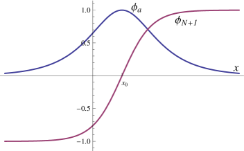
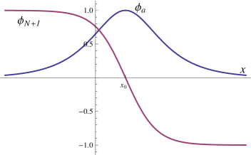
Figure 1: Graphics of $\phi_{a}^{K_{a}}(x)$ (blue) and $\phi_{N+1}^{K_{a}}(x)$ (red) for kink (left) and antikink (right).

4 The moduli space of generic solitary waves

The system of ordinary differential equations (2.6) is the system of motion equations of the repulsive Neumann problem with $N$ degrees of freedom if one interprets the coordinate $y^{1}$ as the “mechanical time” and the field components $\phi_{a}$ as the coordinates setting the “particle position”, the so-called mechanical analogy [10]. It is a well known fact that the Neumann system is Hamilton–Jacobi separable using sphero-conical coordinates [14, 15, 16].

Let us introduce sphero-conical coordinates $(u_{1},u_{2}\dots,u_{N})$ in ${\mathbb{S}}^{N}$ with respect to the set of constants $\bar{\sigma}_{a}^{2}=1-\sigma_{a}^{2}$:

$$\bar{\sigma}_{1}^{2}=0<u_{1}<\bar{\sigma}_{2}^{2}<u_{2}<\cdots<u_{N}<\bar{\sigma}_{N+1}^{2}=1.$$ (4.1)

The Cartesian coordinates in ${\mathbb{R}}^{N+1}$ are given in terms of the sphero-conical coordinates by:

$$\phi_{a}^{2}=u_{0}\frac{U(\bar{\sigma}_{a}^{2})}{B^{\prime}(\bar{\sigma}_{a}^{2})},\qquad U(z)=\prod_{c=1}^{N}(z-u_{c}),\qquad B(z)=\prod_{b=1}^{N+1}\big{(}z-\bar{\sigma}_{b}^{2}\big{)}.$$ (4.2)

The algebraic equation characterizing the ${\mathbb{S}}^{N}$-sphere in ${\mathbb{R}}^{N+1}$ is simply $u_{0}=R^{2}$ in sphero-conical coordinates.

The change of coordinates (4.2) provides a $2^{N+1}$ to $1$ map from the ${\mathbb{S}}^{N}$ sphere to the interior of the hyper-parallelepiped (in the $(u_{1},\dots,u_{N})$ space) ${\mathbb{P}}_{N}$ characterized by the inequalities (4.1). The map from each “$2^{N+1}$-tant” of the ${\mathbb{S}}^{N}$-sphere to the interior of ${\mathbb{P}}_{N}$ is one-to-one. One “$2^{N+1}$-tant” is the piece of ${\mathbb{S}}^{N}$ that lives in each of the $2^{N+1}$ parts in which ${\mathbb{R}}^{N+1}$ is divided by the coordinate $N$-hyperplanes. The intersections of the ${\mathbb{S}}^{N}$-sphere with the coordinate $N$-hyperplanes, $N+1$ ${\mathbb{S}}^{N-1}$-spheres, are $2^{N}$ to $1$ mapped into the boundary of ${\mathbb{P}}_{N}$, a set of $(N-1)$-hyperplanes in the $(u_{1},\dots,u_{N})$ space. Simili modo ${\mathbb{S}}^{N-k}$-spheres, intersection of ${\mathbb{S}}^{N}$ with coordinate $(N-k+1)$-hyperplanes of ${\mathbb{R}}^{N+1}$, are $2^{N-k+1}$ to $1$ mapped into $(N-k)$-hyperplanes of the boundary of ${\mathbb{P}}_{N}$. Finally, the North and South poles of ${\mathbb{S}}^{N}$ are mapped into a single point in the boundary of ${\mathbb{P}}_{N}$: $v^{\pm}\equiv(u_{1}=0,u_{2}=\bar{\sigma}_{2}^{2},\dots,u_{N}=\bar{\sigma}_{N}^{2})$.

The Euclidean metric in ${\mathbb{R}}^{N+1}$ $ds^{2}=d\phi_{1}^{2}+\dots+d\phi_{N+1}^{2}$ becomes in ${\mathbb{P}}_{N}$:

$$\left.ds^{2}\right|_{{\mathbb{S}}^{N}}=\sum_{a=1}^{N}g_{aa}du_{a}^{2},\qquad g_{aa}=\frac{-R^{2}}{4}\frac{U^{\prime}(u_{a})}{B(u_{a})}.$$ (4.3)

Calculations using sphero-conical coordinates remarkably simplify recalling the Jacobi lemma, see e.g. [15]. Let be a collection of $p$ distinct constants $(a_{1},a_{2},\dots a_{p})$, $a_{i}\neq a_{j}$, $\forall\,i\neq j$. Let us define the function $f(z)=\prod\limits_{i=1}^{p}(z-a_{i})$, $p\geq 2$. The following identities hold:

$$\sum_{i=1}^{p}\frac{a_{i}^{k}}{f^{\prime}(a_{i})}=0,\qquad\forall\,k=0,1,\dots,p-2,\qquad\sum_{i=1}^{p}\frac{a_{i}^{p-1}}{f^{\prime}(a_{i})}=1,\qquad\sum_{i=1}^{p}\frac{a_{i}^{p}}{f^{\prime}(a_{i})}=\sum_{i=1}^{p}a_{i}.$$ (4.4)

Now, use of (4.4) allows us easily determine the $V(\vec{\Phi})$ function (2.2) in sphero-conical coordinates:

$$V(u_{1},\dots,u_{n})=\frac{\nu^{2}R^{2}}{2}\left(1-\sum_{a=1}^{N+1}\bar{\sigma}_{a}^{2}+\sum_{b=1}^{N}u_{b}\right).$$

The energy functional for static configurations (3.5) in this system of coordinates can be written as follows:

$$E[u_{1},\dots,u_{N}]=\nu\int dx\left\{\frac{1}{2}\sum_{a=1}^{N}g_{aa}\left(\frac{du_{a}}{dx}\right)^{2}+\frac{R^{2}}{2}\sum_{a=1}^{N}\frac{\prod\limits_{b=1}^{N}(u_{a}-\bar{\sigma}_{b}^{2})}{U^{\prime}(u_{a})}\right\}.$$ (4.5)

The $p-2$ identities on the left in (4.4) allows us to write the potential energy density in different ways. We choose an expression (4.5) in the form of a sum of products in the factors $(u_{a}-\bar{\sigma}_{b}^{2})$ that guarantees a direct verification of the asymptotic conditions (2.7).

Alternatively, the energy can be written in the Bogomolnyi form [18]:

$$E[u_{1},\dots,u_{n}]=\nu\int\frac{dx}{2}\left\{\sum_{a=1}^{N}g_{aa}\left(\frac{du_{a}}{dx}-g^{aa}\frac{\partial W}{\partial u_{a}}\right)^{2}\right\}+\nu\int dx\sum_{a=1}^{N}\frac{\partial W}{\partial u_{a}}\frac{du_{a}}{dx},$$ (4.6)

where $g^{aa}$ denotes the components of the inverse tensor metric, and $W(u_{1},\dots,u_{N})$ is a solution of the partial differential equation:

$$\frac{R^{2}}{2}\sum_{a=1}^{N}\frac{\prod\limits_{b=1}^{N}(u_{a}-\bar{\sigma}_{b}^{2})}{U^{\prime}(u_{a})}=\frac{1}{2}\sum_{a=1}^{N}g^{aa}\left(\frac{\partial W}{\partial u_{a}}\right)^{2}.$$ (4.7)

Note that (4.7) is the “time”-independent Hamilton–Jacobi equation for zero mechanical energy ($i_{1}\equiv 0$) of the “repulsive” Neumann problem. Therefore, $W$ is the zero-energy time-independent characteristic Hamilton function.

The ansatz of separation of variables $W(u_{1},\dots,u_{N})=W_{1}(u_{1})+\dots+W_{N}(u_{N})$ reduces the PDE (4.7) to a set of $N$ uncoupled ordinary differential equations depending on $N$ separation constants $i_{a}$. The separation process is not trivial (see [15]) and requires the use of equations (4.4). Let write explicitly (4.7) as:

$$\sum_{a=1}^{N}\frac{1}{U^{\prime}(u_{a})}\left(\frac{-2B(u_{a})}{R^{2}}(W_{a}^{\prime}(u_{a}))^{2}-\frac{R^{2}}{2}\prod_{b=1}^{N}(u_{a}-\bar{\sigma}_{b}^{2})\right)=i_{1}=0.$$ (4.8)

The identities of the Jacobi lemma (4.4), for $k\leq N-2$, allow to express (4.8) as a system of $N$ equations:

$$\frac{-2B(u_{a})}{R^{2}}(W_{a}^{\prime}(u_{a}))^{2}-\frac{R^{2}}{2}\prod_{b=1}^{N}\big{(}u_{a}-\bar{\sigma}_{b}^{2}\big{)}=i_{2}u_{a}^{N-2}+i_{2}u_{a}^{N-3}+\dots+i_{N-1}u_{a}+i_{N}$$ (4.9)

depending on $N-1$ arbitrary separation constants $i_{2},\dots,i_{N}$.

Asymptotic conditions (2.7) imply, in sphero-conical coordinates, the limits: $\lim\limits_{x\to\pm\infty}u_{a}=\bar{\sigma}_{a}^{2}$. This requirement fixes, in (4.9), all the separation constants $i_{a}$ to be zero, that correspond to the separatrix trajectories between bounded and unbounded motion in the associated mechanical system. Thus, integration of (4.9) gives the $W$ function, i.e. the time-independent, zero mechanical energy, characteristic Hamilton function of the repulsive Neumann problem:

$$W(u_{1},\dots,u_{N})=R^{2}\sum_{a=1}^{N}(-1)^{\delta_{a}}\sqrt{1-u_{a}},\qquad\delta_{a}=0,1.$$ (4.10)

It is interesting to remark that general integration of the Hamilton–Jacobi equation for the Neumann problem involves hyper-elliptic theta-functions [16]. The asymptotic conditions (2.7) guaranteeing finite field theoretical energy to the solitary waves – and finite mechanical action to the associated trajectories – force theta functions in the boundary of the Riemann surface where degenerate to very simple irrational functions.

The ordinary differential equations:

$$\frac{du_{1}}{dx}=g^{11}\frac{\partial W}{\partial u_{1}},\qquad\dots,\qquad\frac{du_{N}}{dx}=g^{NN}\frac{\partial W}{\partial u_{N}}$$ (4.11)

can alternatively be seen as first-order field equations for which the field theoretical energy is of the simple form: $E[u_{1},u_{2},\dots,u_{N}]=\nu\int dW$, see (4.6), or, as the motion equations of the mechanical system restricted to the sub-space of the phase space such that $i_{a}=0$, $\forall\,a=1,2,\dots,N$. In differential form they look:

$$\frac{dx}{U^{\prime}(u_{a})}=\frac{(-1)^{\delta_{a}}du_{a}}{2\sqrt{1-u_{a}}\prod\limits_{b=1}^{n}(u_{a}-\bar{\sigma}_{b}^{2})},\qquad a=1,\dots,N.$$ (4.12)

Although it is possible to integrate equations (4.12) for an arbitrary value of $N$ (see [19] for instance), we shall devote the rest of the paper to analyze the explicit solutions and the structure of the moduli space of solitary waves in the lower $N=2$ and $N=3$ cases.

5 The moduli space of $\boldsymbol{{\mathbb{S}}^{2}}$-solitary waves

5.1 Embedded sine-Gordon kinks on $\boldsymbol{{\mathbb{S}}^{2}}$

  

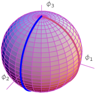
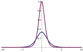
Figure 2: $K_{1}$ (red) and $K_{2}$ (blue) kink orbits over ${\mathbb{S}}^{2}$ (left). Energy densities for $K_{1}/K_{1}^{*}$ (red) and $K_{2}/K_{2}^{*}$ (blue) kinks for a concrete value of $0<\sigma<1$ (right).

There are two sine-Gordon models embedded in the $\phi_{1}=0$ and $\phi_{2}=0$ meridians, see Fig. 2 (left). The non-dimensional parameters, for $N=2$, are: $\sigma_{1}\equiv 1$, $\sigma_{2}\equiv\sigma$ and $\sigma_{3}=0$. The $K_{1}/K_{1}^{*}$ and $K_{2}/K_{2}^{*}$ sine-Gordon kinks/antikinks profiles read:

$$\phi_{1}^{K_{1}}(x)=\frac{R}{\cosh(x-x_{0})},\qquad\phi_{2}^{K_{1}}(x)=0,\qquad\phi_{3}^{K_{1}}(x)=\pm R\tanh(x-x_{0}),$$

$$\phi_{1}^{K_{2}}(x)=0,\qquad\phi_{2}^{K_{2}}(x)=\frac{R}{\cosh\sigma(x-x_{0})},\qquad\phi_{3}^{K_{2}}(x)=\pm R\tanh\sigma(x-x_{0}),$$ (5.1)

$$\phi_{1}^{K_{1}^{*}}(x)=\frac{-R}{\cosh(x-x_{0})},\qquad\phi_{2}^{K_{1}^{*}}(x)=0,\qquad\phi_{3}^{K_{1}^{*}}(x)=\pm R\tanh(x-x_{0}),$$

$$\phi_{1}^{K_{2}^{*}}(x)=0,\qquad\phi_{2}^{K_{2}^{*}}(x)=\frac{-R}{\cosh\sigma(x-x_{0})},\qquad\phi_{3}^{K_{2}^{*}}(x)=\pm R\tanh\sigma(x-x_{0}).$$ (5.2)

The $K_{1}$, $K_{1}^{*}$, $K_{2}$ and $K_{2}^{*}$ kinks belong to ${\cal C}_{\rm NS}$, see Fig. 1; the $\phi_{3}$-component is kink shaped for the four kinks, whereas the $\phi_{1}$- and $\phi_{2}$-components are bell shaped respectively for $K_{1}$ and $K_{2}$ but anti-bell shaped for $K_{1}^{*}$ and $K_{2}^{*}$. The antikinks live in ${\cal C}_{\rm SN}$ and have similar profiles. These solitary waves are topological kinks, and they correspond to heteroclinic trajectories in the analogous mechanical system. Their energies are:

$$E_{K_{1}}=E_{K_{1}^{*}}=2\nu R^{2},\qquad E_{K_{2}}=E_{K_{2}^{*}}=2\nu R^{2}\sigma.$$

The energy of the $K_{1}/K_{1}^{*}$ kinks is greater than the energy of the $K_{2}/K_{2}^{*}$ kinks, see Fig. 2 (right).

5.2 Generic solitary waves on $\boldsymbol{{\mathbb{S}}^{2}}$

We shall denote $(\lambda_{1},\lambda_{2})$ the sphero-conical coordinates in the ${\mathbb{S}}^{2}$-sphere, $\lambda_{0}=R^{2}$, to avoid confusion with the $N=3$ case. In terms of these coordinates the fields read:

$$\phi_{1}^{2}=\frac{R^{2}}{\bar{\sigma}^{2}}\lambda_{1}\lambda_{2},\qquad\phi_{2}^{2}=\frac{R^{2}}{\sigma^{2}\bar{\sigma}^{2}}\big{(}\bar{\sigma}^{2}-\lambda_{1}\big{)}\big{(}\lambda_{2}-\bar{\sigma}^{2}\big{)},\qquad\phi_{3}^{2}=\frac{R^{2}}{\sigma^{2}}(1-\lambda_{1})(1-\lambda_{2}).$$ (5.3)

We recall the definition: $\bar{\sigma}^{2}=1-\sigma^{2}$, and the $(\lambda_{1},\lambda_{2})$ ranges:

$$0<\lambda_{1}<\bar{\sigma}^{2}<\lambda_{2}<1.$$ (5.4)

The change of coordinates (5.3) maps the ${\mathbb{S}}^{2}$-sphere into the interior of the rectangle ${\mathbb{P}}_{2}$ defined by the inequalities (5.4) in the $(\lambda_{1},\lambda_{2})$-plane. In fact, the map is eight to one, due to the squares that appears in (5.3). Each octant of the ${\mathbb{S}}^{2}$-sphere is mapped one to one into the interior of ${\mathbb{P}}_{2}$, whereas the meridians of ${\mathbb{S}}^{2}$ contained in the coordinate planes are mapped into the boundary of ${\mathbb{P}}_{2}$. The set of zeroes ${\cal M}$ of $V(\phi_{1},\phi_{2},\phi_{3})$ in ${\mathbb{S}}^{2}$, the North and South poles, becomes a unique point in ${\mathbb{P}}_{2}$: $v^{\pm}\equiv(\phi_{1},\phi_{2},\phi_{3})=(0,0,\pm R)\Rightarrow v^{\pm}\equiv(\lambda_{1},\lambda_{2})=(0,\bar{\sigma}^{2})$. The quadratic polynomial $V(\phi_{1},\phi_{2},\phi_{3})$ becomes linear in sphero-conical coordinates:

$$V(\lambda_{1},\lambda_{2})=\frac{\nu^{2}R^{2}}{2}\left(\lambda_{1}+\lambda_{2}-\bar{\sigma}^{2}\right)$$

and the energy functional for static configurations in terms of $(\lambda_{1},\lambda_{2})$ is:

$$E[\lambda_{1},\lambda_{2}]=\nu\int dx\left\{\frac{1}{2}\sum_{i=1}^{2}g_{ii}\left(\frac{d\lambda_{i}}{dx}\right)^{2}+\frac{R^{2}}{2}\left(\frac{\lambda_{1}(\lambda_{1}-\bar{\sigma}^{2})}{\lambda_{1}-\lambda_{2}}+\frac{\lambda_{2}(\lambda_{2}-\bar{\sigma}^{2})}{\lambda_{2}-\lambda_{1}}\right)\right\}.$$ (5.5)

Here, the components of the metric tensor (4.3) read:

$$g_{11}=\frac{-R^{2}(\lambda_{1}-\lambda_{2})}{4\lambda_{1}(\bar{\sigma}^{2}-\lambda_{1})(1-\lambda_{1})},\qquad g_{22}=\frac{-R^{2}(\lambda_{2}-\lambda_{1})}{4\lambda_{2}(\bar{\sigma}^{2}-\lambda_{2})(1-\lambda_{2})}.$$

The knowledge of the solution (4.10) for $N=2$:

$$W(\lambda_{1},\lambda_{2})=R^{2}\left((-1)^{\delta_{1}}\sqrt{1-\lambda_{1}}+(-1)^{\delta_{2}}\sqrt{1-\lambda_{2}}\right),\qquad\delta_{1},\delta_{2}=0,1,$$

suggests to write the energy functional (5.5) in the Bogomolnyi form (4.6) leading to the system of first-order ODE’s (4.11):

$$\frac{d\lambda_{1}}{dx}=(-1)^{\delta_{1}}\frac{2\lambda_{1}(\lambda_{1}-\bar{\sigma}^{2})\sqrt{1-\lambda_{1}}}{(\lambda_{1}-\lambda_{2})},\qquad\frac{d\lambda_{2}}{dx}=(-1)^{\delta_{2}}\frac{2\lambda_{2}(\lambda_{2}-\bar{\sigma}^{2})\sqrt{1-\lambda_{2}}}{(\lambda_{2}-\lambda_{1})}.$$

These equations can be separated in a easy way:

$$0=\frac{d\lambda_{1}}{(-1)^{\delta_{1}}2\lambda_{1}(\lambda_{1}-\bar{\sigma}^{2})\sqrt{1-\lambda_{1}}}+\frac{d\lambda_{2}}{(-1)^{\delta_{2}}2\lambda_{2}(\lambda_{2}-\bar{\sigma}^{2})\sqrt{1-\lambda_{2}}},$$ (5.6)

$$dx=\frac{d\lambda_{1}}{(-1)^{\delta_{1}}2(\lambda_{1}-\bar{\sigma}^{2})\sqrt{1-\lambda_{1}}}+\frac{d\lambda_{2}}{(-1)^{\delta_{2}}2(\lambda_{2}-\bar{\sigma}^{2})\sqrt{1-\lambda_{2}}}.$$ (5.7)

The Hamilton–Jacobi procedure precisely prescribes the equation (5.6) as the rule satisfied by the orbits of zero mechanical energy whereas (5.7) sets the mechanical time schedule of these separatrix trajectories between bounded and unbounded motion.

Instead of attempting a direct solution of the system (5.6), (5.7) we introduce new variables $s_{1}=(-1)^{\delta_{1}}\sqrt{1-\lambda_{1}}$, $s_{2}=(-1)^{\delta_{2}}\sqrt{1-\lambda_{2}}$. In terms of $s_{1}$ and $s_{2}$ the ODE’s system (5.6), (5.7), after decomposition in simple fractions, becomes:

$$\sum_{a=1}^{2}\frac{ds_{a}}{1-s_{a}^{2}}=dx,\qquad\sum_{a=1}^{2}\frac{ds_{a}}{\sigma^{2}-s_{a}^{2}}=dx.$$ (5.8)

Integrating equations (5.8) in terms of the inverse of hyperbolic tangents/cotangents, and using the addition formulas for these functions we find the following general solution depending on two real integration constants $\gamma_{1}$ and $\gamma_{2}$:

$$\frac{s_{1}s_{2}}{1+s_{1}s_{2}}=t_{1},\qquad\frac{\sigma^{2}+s_{1}s_{2}}{\sigma(s_{1}+s_{2})}=t_{2},\qquad t_{1}=\tanh(x+\gamma_{1}),\qquad t_{2}=\tanh\sigma(x+\gamma_{2}).$$ (5.9)

To solve the system of equations (5.9) separately in $s_{1}$ and $s_{2}$ we introduce the new variables $A=s_{1}+s_{2}$ and $B=s_{1}s_{2}$. The subsequent linear system in $A$ and $B$ and its solution are:

$$A-t_{1}B=t_{1},\qquad\sigma t_{2}A-B=\sigma^{2},\qquad A=\frac{(1-\sigma^{2})t_{1}}{1-\sigma t_{1}t_{2}},\qquad B=\frac{\sigma t_{1}t_{2}-\sigma^{2}}{1-\sigma t_{1}t_{2}}.$$

Therefore, $s_{1}$ and $s_{2}$ are the roots of the quadratic equation

$$s^{2}-As+B=0,\qquad s_{1}=\frac{A+\sqrt{A^{2}-4B}}{2},\qquad s_{2}=\frac{A-\sqrt{A^{2}-4B}}{2}.$$

Because $\lambda_{1}=1-s_{1}^{2}$, $\lambda_{2}=1-s_{2}^{2}$, the come back to Cartesian coordinates (5.3) provides the explicit analytical formulas for the two-parametric family of solitary waves:

$$\phi_{1}(x)=(-1)^{\epsilon_{1}}R\bar{\sigma}\frac{\mathop{\rm sech}\nolimits(x+\gamma_{1})}{1-\sigma\tanh(x+\gamma_{1})\tanh\sigma(x+\gamma_{2})},\qquad\epsilon_{1}=0,1,$$

$$\phi_{2}(x)=(-1)^{\epsilon_{2}}R\bar{\sigma}\frac{\tanh(x+\gamma_{1})\mathop{\rm sech}\nolimits\sigma(x+\gamma_{2})}{1-\sigma\tanh(x+\gamma_{1})\tanh\sigma(x+\gamma_{2})},\qquad\epsilon_{2}=0,1,$$ (5.10)

$$\phi_{3}(x)=(-1)^{\epsilon_{3}}R\frac{\sigma-\tanh(x+\gamma_{1})\tanh\sigma(x+\gamma_{2})}{1-\sigma\tanh(x+\gamma_{1})\tanh\sigma(x+\gamma_{2})},\qquad\epsilon_{3}=0,1.$$

5.3 The structure of the moduli space of kinks

To describe the structure of the two-dimensional moduli space of solitary waves solutions (5.10) it is convenient to rely on a re-shuffling of the coordinates of the moduli space: $\gamma=-\gamma_{1}$, $\bar{\gamma}=\gamma_{2}-\gamma_{1}$. $\gamma$ determines the “center” of the energy density of a given kink and $\bar{\gamma}$ distinguishes between different kinks in the moduli space by selecting the kink orbit in ${\mathbb{S}}^{2}$, see Figs. 5 and 6. In the Figs. 3 and 4, however, we have plotted the components of the kink profiles for two different choices of $\bar{\gamma}$ and $\gamma=0$. We remark that none of the three components are kink-shaped, the $\phi_{1}$ and $\phi_{3}$ components are bell-shaped and the $\phi_{2}$-components have a maximum and a minimum. The difference is that the $x\to-x$ reflection symmetry is lost for $\bar{\gamma}=5$. The profiles of these two solitary waves tend to the South pole in both $x\to\pm\infty$. Therefore, these kinks are non-topological kinks living in ${\cal C}_{\rm SS}$.

  

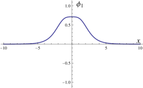
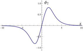
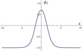
Figure 3: Graphics of (5.10) corresponding to the following values of parameters: $R=1$, $\sigma=0.7$, $\gamma=0$, $\bar{\gamma}=0$, i.e. the maximally symmetric generic kink (it is chosen $\epsilon_{1}=\epsilon_{2}=\epsilon_{3}=0$).

  

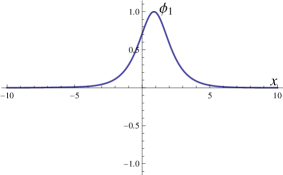
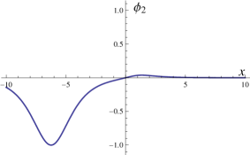
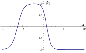
Figure 4: Graphics of (5.10) corresponding to the following values of parameters: $R=1$, $\sigma=0.7$, $\gamma=0$, $\bar{\gamma}=5$, $\epsilon_{1}=\epsilon_{2}=\epsilon_{3}=0$.

($\gamma$, $\bar{\gamma}$) are good coordinates in the solitary wave moduli space characterized by the orbits in ${\mathbb{P}}_{2}$. The inverse mapping to ${\mathbb{S}}^{2}$ is classified by the different choices of $\epsilon_{1}$, $\epsilon_{2}$ and $\epsilon_{3}$:

• The value of $\epsilon_{3}$ selects the topological sector of the solution. Clearly:

  $$\epsilon_{3}=0\Rightarrow\lim_{x\to\pm\infty}\phi_{3}=-R,\qquad\epsilon_{3}=1\Rightarrow\lim_{x\to\pm\infty}\phi_{3}=R$$

  and the equations (5.10) determine two families of non-topological ($NTK$) kinks, one family living in ${\cal C}_{\rm SS}$, $\epsilon_{3}=0$, and the other one belonging to ${\cal C}_{\rm NN}$, $\epsilon_{3}=1$. They are homoclinic trajectories of the analogous mechanical system.

• $\epsilon_{1}=0$ provides the $NTK$ kink orbits running in the $\phi_{1}>0$ hemisphere and $\epsilon_{1}=1$ corresponds to the $NTK$ orbits passing through the other ($\phi_{1}<0$) hemisphere of ${\mathbb{S}}^{2}$.

• $\epsilon_{2}$, however, does not affect to the kink orbit and merely specifies the kink/antikink character of the solitary wave, i.e. the sense in which the orbit is traveled.

    

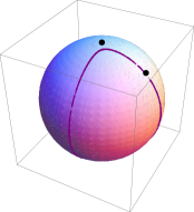
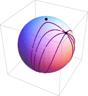
Figure 5: $NTK$ kink-orbits, corresponding to: $R=1$, $\sigma=0.7$, $\epsilon_{1}=\epsilon_{2}=\epsilon_{3}=0$ and $\bar{\gamma}=0$ (left), $\bar{\gamma}=5$ (middle). Several kink orbits in ${\cal C}_{\rm SS}$ corresponding to several different values of $\bar{\gamma}$ (right).

In Fig. 5 (right) several $NTK$ orbits are shown in ${\mathbb{S}}^{2}$. The sector ${\cal C}_{\rm SS}$ and the $\phi_{1}>0$ hemisphere have been selected. All of them cross the $\phi_{2}=0$ meridian at the same point: $F\equiv(R\bar{\sigma},0,R\sigma)$ – in sphero-conical coordinates this point is the low right corner $\lambda_{1}=\lambda_{2}=\bar{\sigma}^{2}$ of ${\mathbb{P}}^{2}$). Therefore the point $F$ is a conjugate point of the South pole S of ${\mathbb{S}}^{2}$.

In Fig. 6 the graphics of the kink energy densities of two members of the $NTK$ family are plotted. We remark that the energy density appears to be composed by two basic elements. This behavior is more evident for $|\bar{\gamma}|\gg 0$ because in such a range the energy density resembles the superposition of the energy densities of the two embedded sine-Gordon kinks (compare with Fig. 2 (right)). All the $NTK$ kinks, however, have the same energy that can be computed from the formula (4.6):

$$E_{NTK}=2\nu R^{2}(1+\sigma)=E_{K_{1}}+E_{K_{2}}.$$

There is a kink energy sum rule: the energy of any $NTK$ kink is exactly the the sum of the two sine-Gordon, $K_{1}$ and $K_{2}$, topological kink energies. These sum rules arises in every field theoretical model with mechanical analogue system which is Hamilton–Jacobi separable and has several unstable equilibrium points, see, e.g., [17]. Moreover, looking at Fig. 4 as a posterior picture to Fig. 3 in a movie that evolves with increasing $\bar{\gamma}$, it is clear that we find almost a $K_{1}$ anti-kink in the $x\gg 0$ region and a $K_{2}^{*}$ kink in the $x\ll 0$ region when $\bar{\gamma}\to\infty$. This means that the solitary waves (5.10) tend to a $K_{1}$ kink/antikink plus a $K_{2}$ antikink/kink when $\bar{\gamma}\to\pm\infty$. Thus the combinations $K_{1}+K_{2}$ (kink/antikink and antikink/kink) form the closure of the $NTK$ moduli space and belong to the boundary. Alternatively, one can tell that there exist only two basic (topological) kink solutions and the rest of the kinks, the $NTK$ family, are (nonlinear) combinations of the two basic solitary waves.

 

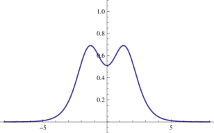
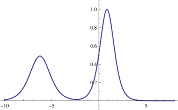
Figure 6: Kink energy density for the $NTK$ determined by the constants: $R=1$, $\sigma=0.7$, and $\gamma=\bar{\gamma}=0$ (left), $\gamma=0$ and $\bar{\gamma}=5$ (right).

6 The moduli space of $\boldsymbol{{\mathbb{S}}^{3}}$-solitary waves

6.1 Embedded $\boldsymbol{N=2}$ kinks

In the massive nonlinear ${\mathbb{S}}^{3}$-sigma model we first count the three embedded sine-Gordon kinks:

• The $K_{1}/K_{1}^{*}$ kinks and their anti-kinks living in the meridian

  $$\left\{\phi_{1}^{2}+\phi_{4}^{2}=R^{2}\right\}\equiv\left\{\{\phi_{2}=\phi_{3}=0\}\bigcap\left\{\phi_{1}^{2}+\phi_{2}^{2}+\phi_{3}^{2}+\phi_{4}^{2}=R^{2}\right\}\right\},$$

  the intersection of the $\phi_{2}=\phi_{3}=0$ plane with the ${\mathbb{S}}^{3}$ sphere.

• Idem for the $K_{2}/K_{2}^{*}$ and their anti-kinks:

  $$\left\{\phi_{2}^{2}+\phi_{4}^{2}=R^{2}\right\}\equiv\left\{\{\phi_{1}=\phi_{3}=0\}\bigcap\left\{\phi_{1}^{2}+\phi_{2}^{2}+\phi_{3}^{2}+\phi_{4}^{2}=R^{2}\right\}\right\}.$$

• Idem for the $K_{3}/K_{3}^{*}$ kinks and their anti-kinks:

  $$\left\{\phi_{3}^{2}+\phi_{4}^{2}=R^{2}\right\}\equiv\left\{\{\phi_{1}=\phi_{2}=0\}\bigcap\left\{\phi_{1}^{2}+\phi_{2}^{2}+\phi_{3}^{2}+\phi_{4}^{2}=R^{2}\right\}\right\}.$$

The novelty is that all the non-topological kinks of the massive nonlinear ${\mathbb{S}}^{2}$-sigma model are embedded in the ${\mathbb{S}}^{3}$ version in three different ${\mathbb{S}}^{2}$ “meridian” sub-manifolds.

1. Consider the two-dimensional ${\mathbb{S}}^{2}_{I}$ sphere:

   $$\left\{\phi_{2}^{2}+\phi_{3}^{2}+\phi_{4}^{2}=R^{2}\right\}\equiv\left\{\{\phi_{1}=0\}\bigcap\left\{\phi_{1}^{2}+\phi_{2}^{2}+\phi_{3}^{2}+\phi_{4}^{2}=R^{2}\right\}\right\},$$

   the intersection of the $\phi_{1}=0$ 3-hyperplane in ${\mathbb{R}}^{4}$ with the ${\mathbb{S}}^{3}$-sphere.

   The restriction of the $N=3$-model to these two-manifold collects all the solitary waves of the $N=2$-model. We shall call $NTK_{I}$ kinks to the $N=2$ $NTK$ kinks of the $N=2$ model that lives in ${\mathbb{S}}^{2}_{I}$. The $K_{2}/K_{2}^{*}$ and $K_{3}/K_{3}^{*}$ sine-Gordon topological kinks/anti-kinks also live in in ${\mathbb{S}}^{2}_{I}$ and belong to the boundary of the $NTK_{I}$ moduli space.

2. Idem for the ${\mathbb{S}}^{2}_{II}$ sphere:

   $$\left\{\phi_{1}^{2}+\phi_{3}^{2}+\phi_{4}^{2}=R^{2}\right\}\equiv\left\{\{\phi_{2}=0\}\bigcap\left\{\phi_{1}^{2}+\phi_{2}^{2}+\phi_{3}^{2}+\phi_{4}^{2}=R^{2}\right\}\right\}.$$

   The non-topological kinks running on this 2-sphere will be termed $NTK_{II}$. The sine-Gordon kinks/antikinks are: $K_{1}/K_{1}^{*}$ and $K_{3}/K_{3}^{*}$.

3. Idem for the ${\mathbb{S}}^{2}_{III}$ sphere:

   $$\left\{\phi_{1}^{2}+\phi_{2}^{2}+\phi_{4}^{2}=R^{2}\right\}\equiv\left\{\{\phi_{3}=0\}\bigcap\left\{\phi_{1}^{2}+\phi_{2}^{2}+\phi_{3}^{2}+\phi_{4}^{2}=R^{2}\right\}\right\}.$$

   The non-topological kinks running on this 2-sphere will be termed $NTK_{III}$. The sine-Gordon kinks/antikinks are: $K_{1}/K_{1}^{*}$ and $K_{2}/K_{2}^{*}$.

In the “equatorial” sphere $\phi_{1}^{2}+\phi_{2}^{2}+\phi_{3}^{2}=R^{2}$, $\phi_{4}=0$, of ${\mathbb{S}}^{3}$, however, there are no kinks because the equilibrium points, the North and South poles, are not included.

6.2 Generic solitary waves

Away from the meridian 2-spheres ${\mathbb{S}}^{2}_{I}$, ${\mathbb{S}}^{2}_{II}$ and ${\mathbb{S}}^{2}_{III}$ considered in the previous sub-section, there is a three-parametric family of generic kinks. In $N=3$ dimensional sphero-conical coordinates (4.2):

$$\phi_{1}^{2}=u_{0}\frac{u_{1}u_{2}u_{3}}{\bar{\sigma}_{2}^{2}\bar{\sigma}_{3}^{2}},\qquad\phi_{2}^{2}=u_{0}\frac{(\bar{\sigma}_{2}^{2}-u_{1})(\bar{\sigma}_{2}^{2}-u_{2})(\bar{\sigma}_{2}^{2}-u_{3})}{\sigma_{2}^{2}\bar{\sigma}_{2}^{2}(\bar{\sigma}_{3}^{2}-\bar{\sigma}_{2}^{2})},$$

$$\phi_{3}^{2}=u_{0}\frac{(\bar{\sigma}_{3}^{2}-u_{1})(\bar{\sigma}_{3}^{2}-u_{2})(\bar{\sigma}_{3}^{2}-u_{3})}{\sigma_{3}^{2}\bar{\sigma}_{3}^{2}(\bar{\sigma}_{2}^{2}-\bar{\sigma}_{3}^{2})},\qquad\phi_{4}^{2}=u_{0}\frac{(1-u_{1})(1-u_{2})(1-u_{3})}{\sigma_{2}^{2}\sigma_{3}^{2}},$$ (6.1)

such that: $0<u_{1}<\bar{\sigma}_{2}^{2}<u_{2}<\bar{\sigma}_{3}^{2}<u_{3}<1$, the ${\mathbb{S}}^{3}$-sphere of radius $R$ is characterized by the equation: $u_{0}=R^{2}$. The change of coordinates (6.1) corresponds to a sixteen-to-one map from the points of ${\mathbb{S}}^{3}$ out of the coordinate 3-hyperplanes $\phi_{a}=0$, $a=1,\dots,4$, to the interior of the parallelepiped ${\mathbb{P}}_{3}$, in the $(u_{1},u_{2},u_{3})$-space, defined by the inequalities above. The meridian 2-spheres are eight-to-one mapped into the boundary of ${\mathbb{P}}_{3}$, where some inequalities become identities: $u_{1}=0$ for ${\mathbb{S}}^{2}_{I}$, $\{u_{1}=\bar{\sigma}_{2}^{2}\}\bigcup\{u_{2}=\bar{\sigma}_{2}^{2}\}$, for ${\mathbb{S}}_{II}$, and $\{u_{2}=\bar{\sigma}_{3}^{2}\}\bigcup\{u_{3}=\bar{\sigma}_{3}^{2}\}$ in the ${\mathbb{S}}^{2}_{III}$ case. The one-dimensional coordinate meridians of these 2-spheres, in particular those that are the embedded sine-Gordon kink orbits are four-to-one mapped into the edges of ${\mathbb{P}}_{3}$, see Fig. 7. Finally, the North and South poles of ${\mathbb{S}}^{3}$ are two-to-one mapped into one vertex of ${\mathbb{P}}_{3}$: $v^{\pm}\equiv(u_{1},u_{2},u_{3})=(0,\bar{\sigma}_{2}^{2},\bar{\sigma}_{3}^{2})$.

  

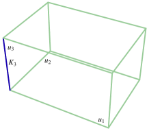
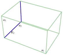
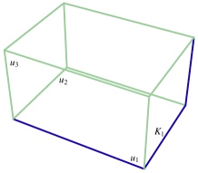
Figure 7: Parallelepiped ${\mathbb{P}}_{3}$. The $K_{1}$, $K_{2}$ and $K_{3}$ sine-Gordon kink orbits are depicted (in blue) at the corresponding edges of ${\mathbb{P}}_{3}$.

The quadratic polynomial $V(\phi_{1},\phi_{2},\phi_{3},\phi_{4})$ becomes linear in the sphero-conical coordinates:

$$V(u_{1},u_{2},u_{3})=\frac{\nu^{2}R^{2}}{2}\left(u_{1}+u_{2}+u_{3}-\bar{\sigma}_{2}^{2}-\bar{\sigma}_{3}^{2}\right),$$

but we write it in “separable” form:

$$V(u_{1},u_{2},u_{3})=\frac{\nu^{2}R^{2}}{2}\left(\frac{u_{1}(u_{1}-\bar{\sigma}_{2}^{2})(u_{1}-\bar{\sigma}_{3}^{2})}{(u_{1}-u_{2})(u_{1}-u_{3})}\right.$$

$$\left.\phantom{V(u_{1},u_{2},u_{3})=}{}+\frac{u_{2}(u_{2}-\bar{\sigma}_{2}^{2})(u_{2}-\bar{\sigma}_{3}^{2})}{(u_{2}-u_{1})(u_{2}-u_{3})}+\frac{u_{3}(u_{3}-\bar{\sigma}_{2}^{2})(u_{3}-\bar{\sigma}_{3}^{2})}{(u_{3}-u_{1})(u_{3}-u_{2})}\right).$$

The reason is that in this form it is obvious that the PDE (4.7) reduces to the system of three uncoupled ODE that can be immediately integrated to find (4.10):

$$W(u_{1},u_{2},u_{3})=R^{2}\left((-1)^{\delta_{1}}\sqrt{1-u_{1}}+(-1)^{\delta_{2}}\sqrt{1-u_{2}}\right.$$

$$\left.\phantom{W(u_{1},u_{2},u_{3})=}{}+(-1)^{\delta_{3}}\sqrt{1-u_{3}}\right),\qquad\delta_{1},\delta_{2},\delta_{3}=0,1.$$

The Bogomolnyi splitting of the energy (4.6) prompts the first-order equations (4.11):

$$\frac{dx}{U^{\prime}(u_{a})}=\frac{(-1)^{\delta_{a}}du_{a}}{2u_{a}(u_{a}-\bar{\sigma}_{2}^{2})(u_{a}-\bar{\sigma}_{3}^{2})\sqrt{1-u_{a}}},\qquad a=1,2,3.$$ (6.2)

It is convenient to pass to the variables:

$$s_{1}=(-1)^{\delta_{1}}\sqrt{1-u_{1}},\qquad s_{2}=(-1)^{\delta_{2}}\sqrt{1-u_{2}},\qquad s_{3}=(-1)^{\delta_{3}}\sqrt{1-u_{3}}$$

because the quadratures in (6.2) become:

$$\sum_{a=1}^{3}\frac{ds_{a}}{1-s_{a}^{2}}=-dx,\qquad\sum_{a=1}^{3}\frac{ds_{a}}{\sigma_{2}^{2}-s_{a}^{2}}=-dx,\qquad\sum_{a=1}^{3}\frac{ds_{a}}{\sigma_{3}^{2}-s_{a}^{2}}=-dx,$$ (6.3)

where only enter rational functions. The integration of (6.3) is straightforward:

$$\mathop{\rm arctanh}\nolimits s_{1}+\mathop{\rm arctanh}\nolimits s_{2}+\mathop{\rm arctanh}\nolimits s_{3}=-(x+\gamma_{1}),$$

$$\mathop{\rm arccoth}\nolimits\frac{s_{1}}{\sigma_{2}}+\mathop{\rm arctanh}\nolimits\frac{s_{2}}{\sigma_{2}}+\mathop{\rm arctanh}\nolimits\frac{s_{3}}{\sigma_{2}}=-\sigma_{2}(x+\gamma_{2}),$$ (6.4)

$$\mathop{\rm arccoth}\nolimits\frac{s_{1}}{\sigma_{3}}+\mathop{\rm arccoth}\nolimits\frac{s_{2}}{\sigma_{3}}+\mathop{\rm arctanh}\nolimits\frac{s_{3}}{\sigma_{3}}=-\sigma_{3}(x+\gamma_{3}).$$

The addition formulas for the inverse hyperbolic functions, and the definition of “Vieta variables”:

$$A=s_{1}+s_{2}+s_{3},\qquad B=s_{1}s_{2}+s_{1}s_{3}+s_{2}s_{3},\qquad C=s_{1}s_{2}s_{3}$$

reduce the system of transcendent equations (6.4) to the linear system:

$$A-t_{1}B+C=t_{1},$$

$$\sigma_{2}^{2}t_{2}A-\sigma_{2}B+t_{2}C=\sigma_{2}^{3},$$

$$\sigma_{3}^{2}A-\sigma_{3}t_{3}B+C=\sigma_{3}^{3}t_{3},$$

where: $t_{1}=\tanh(-(x+\gamma_{1}))$, $t_{2}=\tanh(-\sigma_{2}(x+\gamma_{2}))$, $t_{3}=\tanh(-\sigma_{3}(x+\gamma_{3}))$. From the solutions $A$, $B$ and $C$ of this linear system we obtain the $s_{1}$, $s_{2}$ and $s_{3}$ variables as the roots of the cubic equation:

$$s^{3}-As^{2}+Bs-C=0.$$

The standard Cardano parameters

$$q=\frac{B}{3}-\frac{A^{2}}{9},\qquad r=\frac{1}{6}(3C-AB)+\frac{A^{3}}{27},\qquad\theta=\arccos\frac{-r}{\sqrt{-q^{3}}}$$

provide the three roots $s_{1}$, $s_{2}$ and $s_{3}$ by Cardano’s formulas, and recalling that: $u_{a}=1-s_{a}^{2}$, $a=1,2,3$ we finally obtain:

$$u_{1}(x)=1-\left(\frac{A}{3}+2\sqrt{-q}\cos\frac{\theta}{3}\right)^{2},$$

$$u_{2}(x)=1-\left(\frac{A}{3}+\sqrt{-q}\left(-\cos\frac{\theta}{3}-\sqrt{3}\sin\frac{\theta}{3}\right)\right)^{2},$$ (6.5)

$$u_{3}(x)=1-\left(\frac{A}{3}+\sqrt{-q}\left(-\cos\frac{\theta}{3}+\sqrt{3}\sin\frac{\theta}{3}\right)\right)^{2},$$

which in turn can be mapped back to cartesian coordinates. The explicit analytical expressions for the generic kinks are:

$$\begin{split}&\phi_{1}(x)=(-1)^{\epsilon_{1}}R\bar{\sigma}_{2}\bar{\sigma}_{3}\frac{\left(\sigma_{2}-\sigma_{3}t_{2}t_{3}\right)\mathop{\rm sech}\nolimits(x+\gamma_{1})}{\sigma_{2}\bar{\sigma}_{3}^{2}-(\sigma_{2}^{2}-\sigma_{3}^{2})t_{1}t_{2}-\sigma_{3}\bar{\sigma}_{2}^{2}t_{2}t_{3}},\\ &\phi_{2}(x)=(-1)^{\epsilon_{2}}R\bar{\sigma}_{2}\sqrt{\sigma_{2}^{2}-\sigma_{3}^{2}}\frac{\left(t_{1}-\sigma_{3}t_{3}\right)\mathop{\rm sech}\nolimits\sigma_{2}(x+\gamma_{2})}{\displaystyle\sigma_{2}\bar{\sigma}_{3}^{2}-(\sigma_{2}^{2}-\sigma_{3}^{2})t_{1}t_{2}-\sigma_{3}\bar{\sigma}_{2}^{2}t_{2}t_{3}},\\ &\phi_{3}(x)=(-1)^{\epsilon_{3}}R\bar{\sigma}_{3}\sqrt{\sigma_{2}^{2}-\sigma_{3}^{2}}\frac{\left(\sigma_{2}-t_{1}t_{2}\right)\mathop{\rm sech}\nolimits\sigma_{3}(x+\gamma_{3})}{\sigma_{2}\bar{\sigma}_{3}^{2}-(\sigma_{2}^{2}-\sigma_{3}^{2})t_{1}t_{2}-\sigma_{3}\bar{\sigma}_{2}^{2}t_{2}t_{3}},\\ &\phi_{4}(x)=(-1)^{\epsilon_{4}}R\frac{-\bar{\sigma}_{2}^{2}\sigma_{3}t_{1}-\left(\sigma_{2}^{2}-\sigma_{3}^{2}-\sigma_{2}\bar{\sigma}_{3}^{2}t_{1}t_{2}\right)t_{3}}{\sigma_{2}\bar{\sigma}_{3}^{2}-(\sigma_{2}^{2}-\sigma_{3}^{2})t_{1}t_{2}-\sigma_{3}\bar{\sigma}_{2}^{2}t_{2}t_{3}},\end{split}$$ (6.6)

where $\epsilon_{a}=0,1$, $\forall\,a=1,\dots,4$. Equations (6.6) define a three-parameter family of kinks in the ${\mathbb{S}}^{3}$-sphere.

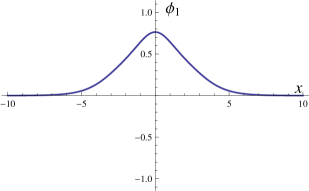
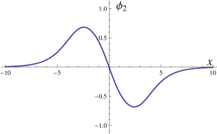
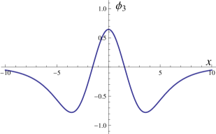
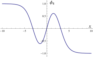
Figure 8: Graphics of the kink solutions (6.6) for the following values of the parameters: $R=1$, $\sigma_{2}=\frac{3}{4}$, $\sigma_{3}=\frac{1}{2}$, $\gamma_{1}=\gamma_{2}=\gamma_{3}=0$, $\epsilon_{a}=0$, $\forall\,a=1,\dots,4$. This maximally symmetric kink.

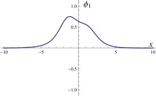
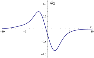
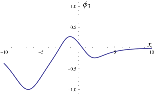
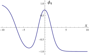
Figure 9: Graphics of (6.6) for: $R=1$, $\sigma_{2}=\frac{3}{4}$, $\sigma_{3}=\frac{1}{2}$, $\gamma_{1}=0.8$, $\gamma_{2}=1$, $\gamma_{3}=4$, $\epsilon_{a}=0$, $\forall\,a=1,\dots,4$.

6.3 The structure of the moduli space of kinks

In the Figs. 8 and 9 two generic kink profiles have been plotted for representative values of the parameters.

A glance to the plots of $\phi_{4}$ as function of $x$ shows that the kinks are topological interpolating between the North and the South poles. In fact, all the generic kinks are topological. The analysis of the asymptotic behavior of the fourth field component in (6.6) determines the topological character of all the solitary waves solutions. The generic kinks belong to either the ${\cal C}_{\rm NS}$ or the ${\cal C}_{\rm SN}$ sectors of the configuration space. The limits

$$\begin{split}&\lim_{x\to-\infty}\left(\phi_{1}(x),\phi_{2}(x),\phi_{3}(x),\phi_{4}(x)\right)=(0,0,0,(-1)^{\epsilon_{4}}R),\\ &\lim_{x\to\infty}\left(\phi_{1}(x),\phi_{2}(x),\phi_{3}(x),\phi_{4}(x)\right)=(0,0,0,-(-1)^{\epsilon_{4}}R)\end{split}$$

show that $\epsilon_{4}=0$ implies that the $TK$ kink family lies in ${\cal C}_{\rm NS}$, whereas $\epsilon_{4}=1$ sends the $TK$ family to live in ${\cal C}_{\rm SN}$. The other sign options, $(-1)^{\epsilon_{1}}$, $(-1)^{\epsilon_{2}}$ and $(-1)^{\epsilon_{3}}$, determine the three-dimensional hemispheres accommodating the different $TK$ kink orbits, as well as the kink/antikink character of the solutions, in a smooth generalization of the $N=2$ $NTK$ kinks.

  

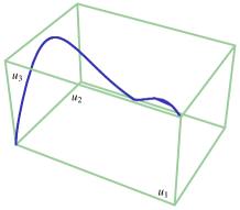
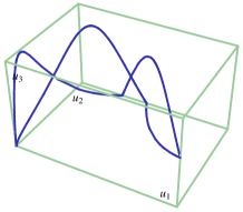
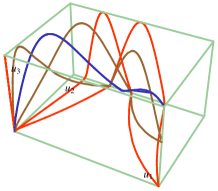
Figure 10: $TK$ orbit corresponding to: $\gamma_{1}=\gamma_{2}=\gamma_{3}=0$ (left). The case: $\gamma_{1}=0.8$, $\gamma_{2}=2$ and $\gamma_{3}=2$ (middle). Three orbits corresponding to different values of the parameters (right).

It is possible to draw the kink orbits in the ${\mathbb{P}}_{3}$ parallelepiped using the solutions (6.5) in sphero-conical coordinates. In the Fig. 10 (right) several $TK$ orbits are drawn together. The energy of all the $TK$ kinks is:

$$E_{TK}=2\nu R^{2}(1+\sigma_{2}+\sigma_{3})=E_{K_{1}}+E_{K_{2}}+E_{K_{3}}.$$

There is a new kink energy sum rule specifically arising in the $N=3$ model. In the Fig. 11 it can be viewed how the energy density reflects this energy sum rule: the energy density of a given member of the $TK$ family is a “composition” of the energy densities of the sine-Gordon kinks $K_{1}$, $K_{2}$ and $K_{3}$, see Fig. 11 (middle) and (right). This structure is completely similar to the kink manifold of the field theoretical model with target space flat ${\mathbb{R}}^{3}$ and the Garnier system as mechanical analogue problem, see [13] and [17]. In fact, the equations are identical, even thought in that case the problem is separable using elliptical coordinates in ${\mathbb{R}}^{3}$, [13, 17]. The calculation of the limits of the $TK$ family when the parameters $\gamma_{1}$, $\gamma_{2}$ and $\gamma_{3}$ tend to $\pm\infty$ is not a simple task, but it is possible to show that all the possibilities arising from the energy sum rule are obtained for the different limits (see [17] for details; the model is different but the equations are the same and thus the analytical calculation of the limiting cases coincides). In the Fig. 10 (right), for instance, a $TK$ kink orbit (in red color) close to the limiting combination $K_{3}$ plus a member of the $NTK_{III}$ family, is plotted.

Finally, the structure of the kink manifolds for the $N=2$ and $N=3$ models allows us to foresee that in higher $N$, the generic kinks will be topological if $N$ is an odd number, and non-topological for even $N$. In fact, the kink energy sum rule will establish that the energy of a generic solitary wave is the sum of the energies of the $N$ sine-Gordon kinks embedded in the model.

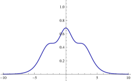
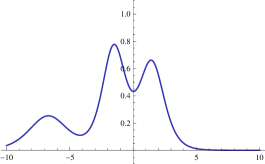
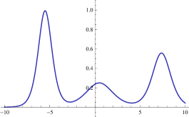
Figure 11: Kink energy densities for different values of the constants $\gamma_{1}$, $\gamma_{2}$ and $\gamma_{3}$.

7 Kink stability

The analysis of the kink stability requires the study of the small fluctuations around kinks. For simplicity, we will only present the explicit results for the topological kinks of the ${\mathbb{S}}^{2}$ model, and also a geometrical analysis in terms of Jacobi fields that allows us to demonstrate the instability of the non-topological kinks. The generalization to the arbitrary $N$ case is straightforward.

7.1 Small fluctuations on topological kinks, $\boldsymbol{K_{1}}$ and $\boldsymbol{K_{2}}$

Taking into account the explicit expressions of the $K_{1}$ and $K_{2}$ sine-Gordon kinks of the ${\mathbb{S}}^{2}$ model, we will use spherical coordinates in ${\mathbb{S}}^{2}$ in order to alleviate the notation. Thus we introduce the coordinates:

$$\phi=R\sin\theta^{1}\cos\theta^{2},\qquad\phi_{2}=R\sin\theta^{1}\sin\theta^{2},\qquad\phi_{3}=R\cos\theta^{1}$$

with $\theta^{1}\in[0,\pi]$, $\theta^{2}\in[0,2\pi)$. The metric tensor over ${\mathbb{S}}^{2}$ is written now as: $ds^{2}=R^{2}d\theta^{1}d\theta^{1}+R^{2}\sin^{2}\theta^{1}d\theta^{2}d\theta^{2}$. The associated Christoffel symbols and Riemann curvature tensor components will be:

$$\Gamma^{1}_{22}=-\frac{1}{2}\sin 2\theta^{1},\qquad\Gamma^{2}_{12}=\Gamma^{2}_{21}=\mathop{\rm cotan}\nolimits\theta^{1},$$

$$R^{1}_{212}=-R^{1}_{122}={\rm sin}^{2}\theta^{1},\qquad R^{2}_{121}=-R^{2}_{211}=1.$$

The analysis of small fluctuations around a kink $\theta_{K}(x)\equiv(\theta_{K}^{1}(x),\theta_{K}^{2}(x))$ is determined by the second-order Hessian operator:

$$\Delta_{K}\eta=-\big{(}\nabla_{\theta_{K}^{\prime}}\nabla_{\theta_{K}^{\prime}}\eta+R(\theta^{\prime}_{K},\eta)\theta^{\prime}_{K}+\nabla_{\eta}{\rm grad}\,V\big{)},$$ (7.1)

i.e. the geodesic deviation operator plus the Hessian of the potential energy density, valuated at the kink. $\eta$ denotes the perturbation around the kink. Let $\theta(x)$ denote the deformed trajectory, $\theta(x)=\theta_{K}(x)+\eta(x)$, with $\eta(x)=(\eta^{1}(x),\eta^{2}(x))$, then we introduce the following contra-variant vector fields along the kink trajectory, $\eta,\theta^{\prime}_{K}\in\Gamma(T{\mathbb{S}}^{2}\left|{}_{K}\right.)$:

$$\eta(x)=\eta^{1}(x)\frac{\partial}{\partial\theta^{1}}+\eta^{2}(x)\frac{\partial}{\partial\theta^{2}},\qquad\theta^{\prime}_{K}(x)=\theta_{K}^{\prime 1}\frac{\partial}{\partial\theta^{1}}+\theta_{K}^{\prime 2}\frac{\partial}{\partial\theta^{2}}.$$

We will use standard notation for covariant derivatives and Riemann tensor:

$$\nabla_{\theta_{K}^{\prime}}\eta=\big{(}\eta^{\prime i}(x)+\Gamma^{i}_{jk}\eta^{j}\theta_{K}^{\prime k}\big{)}\frac{\partial}{\partial\theta^{i}},\qquad R(\theta^{\prime}_{K},\eta)\theta^{\prime}_{K}=\theta_{K}^{\prime i}\eta^{j}(x)\theta_{K}^{\prime k}R^{l}_{ijk}\frac{\partial}{\partial\theta^{l}}.$$

The geodesic deviation operator and the Hessian of the potential read:

$$\frac{D^{2}\eta}{dx^{2}}+R(\theta^{\prime}_{K},\eta)\theta^{\prime}_{K}=\nabla_{\theta_{K}^{\prime}}\nabla_{\theta_{K}^{\prime}}\eta+R(\theta^{\prime}_{K},\eta)\theta^{\prime}_{K},$$

$$\nabla_{\eta}\,{\rm grad}\,V=\eta^{i}\left(\frac{\partial^{2}V}{\partial\theta^{i}\partial\theta^{j}}-\Gamma^{k}_{ij}\frac{\partial V}{\partial\theta^{k}}\right)g^{jl}\frac{\partial}{\partial\theta^{l}}$$

evaluated at $\theta_{K}(x)$. In sum, second-order kink fluctuations are determined by the operator:

$$\Delta_{K}\eta=-\left(\frac{D^{2}\eta}{dx^{2}}+R(\theta^{\prime}_{K},\eta)\theta^{\prime}_{K}+\nabla_{\eta}\,{\rm grad}\,V\right)$$

$$\phantom{\Delta_{K}\eta}{}=-\left(\frac{d^{2}\eta^{1}}{dx^{2}}-\cos 2\theta_{K}^{1}\left[\big{(}\theta_{K}^{\prime 2}\big{)}^{2}+\sigma^{2}+\bar{\sigma}^{2}\cos^{2}\theta_{K}^{2}\right]\eta^{1}-\sin 2\theta_{K}^{1}\theta_{K}^{\prime 2}\frac{d\eta^{2}}{dx}\right.$$

$$\left.\phantom{\Delta_{K}\eta=}{}-\left[\big{(}1+\cos 2\theta_{K}^{1}\big{)}\theta_{K}^{\prime 1}\theta_{K}^{\prime 2}+\frac{\sin 2\theta_{K}^{1}}{2}\left(\theta_{K}^{\prime\prime 2}-\bar{\sigma}^{2}\frac{\sin 2\theta_{K}^{2}}{2}\right)\right]\eta^{2}\right)\frac{\partial}{\partial\theta^{1}}$$

$$\phantom{\Delta_{K}\eta=}{}-\left(2\mathop{\rm cotan}\nolimits\theta_{K}^{1}\theta_{K}^{\prime 2}\frac{d\eta^{1}}{dx}+\big{(}\mathop{\rm cotan}\nolimits\theta_{K}^{1}\theta_{K}^{\prime\prime 2}-\theta_{K}^{\prime 1}\theta_{K}^{\prime 2}\big{)}\eta^{1}+\frac{d^{2}\eta^{2}}{dx^{2}}\right.$$

$$\left.\phantom{\Delta_{K}\eta=}{}+2\mathop{\rm cotan}\nolimits\theta_{K}^{1}\theta_{K}^{\prime 1}\frac{d\eta^{2}}{dx}+\big{(}\mathop{\rm cotan}\nolimits\theta_{K}^{1}\theta_{K}^{\prime\prime 1}-(\theta_{K}^{\prime 1})^{2}-\cos^{2}\theta_{K}^{1}\big{(}\theta_{K}^{\prime 2}\big{)}^{2}\big{)}\right)\frac{\partial}{\partial\theta^{2}}.$$ (7.2)

The spectrum of small fluctuations around $\boldsymbol{K_{2}/K_{2}^{*}}$ kinks. The $K_{2}/K_{2}^{*}$ kink solutions (5.1), (5.2) are written, in spherical coordinates, as follows:

$$\theta_{K_{2}}^{1}=2\arctan e^{\pm\sigma(x-x_{0})},\qquad\theta_{K_{2}}^{2}=\frac{\pi}{2},$$

$$\theta_{K_{2}^{*}}^{1}=2\arctan e^{\pm\sigma(x-x_{0})},\qquad\theta_{K_{2}^{*}}^{2}=\frac{3\pi}{2},$$

where the $(\pm)$ sign determine the kink/antikink choice, and we will take $x_{0}=0$ for simplicity. Plugging these $K_{2}/K_{2}^{*}$ kink solutions in (7.2), we obtain the differential operator acting on the second-order fluctuation operator around the $K_{2}/K_{2}^{*}$ kinks:

$$\Delta_{K_{2}}\eta=\left[-\frac{d^{2}\eta^{1}}{dx^{2}}+\left(\sigma^{2}\!-\frac{2\sigma^{2}}{{\rm cosh}^{2}\sigma x}\right)\!\eta^{1}\right]\frac{\partial}{\partial\theta^{1}}+\left[-\frac{d^{2}\eta^{2}}{dx^{2}}+2\sigma{\rm tanh}\sigma x\frac{d\eta^{2}}{dx}+\bar{\sigma}^{2}\eta^{2}\right]\frac{\partial}{\partial\theta^{2}}.\!\!\!$$ (7.3)

We know from classical differential geometry that this expression can be simplified if one uses a parallel basis along the kink trajectory. Therefore let us consider the equations of parallel transport along $K_{2}$ kinks: $\nabla_{\theta_{K_{2}}^{\prime}}v=0$, where $v$ is the vector-field: $v(x)=v^{1}(x)\frac{\partial}{\partial\theta^{1}}+v^{2}(x)\frac{\partial}{\partial\theta^{2}}$. These equations are written explicitly as:

$$\frac{dv^{i}}{dx}+\Gamma^{i}_{jk}\bar{\theta}^{\prime j}v^{k}=0\Rightarrow\left\{\begin{array}[]{ll}\displaystyle\frac{dv^{1}}{dx}=0&\Rightarrow\ v^{1}(x)=1,\vspace{2mm}\\ \displaystyle\frac{dv^{2}}{dx}+\sigma\frac{\mathop{\rm cotan}\nolimits(2\arctan e^{\sigma x})}{\cosh\sigma x}v^{2}=0&\Rightarrow\ v^{2}(x)=\cosh\sigma x.\end{array}\right.$$

Therefore the vector-fields: $v_{1}=\frac{\partial}{\partial\theta^{1}}$ and $v_{2}(x)=\cosh\sigma x\frac{\partial}{\partial\theta^{2}}$ form a frame $\left\{v_{1},v_{2}\right\}$ in $\Gamma(T{\mathbb{S}}^{2}|_{K_{2}})$ parallel to the $K_{2}$ kink in which (7.3) reads as follows:

$$\Delta_{K_{2}}\eta=\Delta_{K_{2}^{*}}\eta=\left[-\frac{d^{2}\bar{\eta}^{1}}{dx^{2}}+\left(\sigma^{2}-\frac{2\sigma^{2}}{\cosh^{2}\sigma x}\right)\bar{\eta}^{1}\right]v_{1}+\left[-\frac{d^{2}\bar{\eta}^{2}}{dx^{2}}+\left(1-\frac{2\sigma^{2}}{\cosh^{2}\sigma x}\right)\bar{\eta}^{2}\right]v_{2},$$

where $\eta=\bar{\eta}^{1}v_{1}+\bar{\eta}^{2}v_{2}$, $\eta^{1}=\bar{\eta}^{1}$, and $\eta^{2}=\cosh\sigma x\bar{\eta}^{2}$. Thus the second-order fluctuation operator, expressed in the parallel frame, is a diagonal matrix of transparent Pösch–Teller Schrödinger operators with very well known spectra. In fact, in the $v_{1}=\frac{\partial}{\partial\theta^{1}}$ direction we find the Schrödinger operator governing sine-Gordon kink fluctuations, as could be expected. The novelty is that we find another Pösch–Teller potential of the same type in the $v_{2}=\frac{\partial}{\partial\theta^{2}}$ direction, orthogonal to the kink trajectory. The spectra is given by:

• $v_{1}$ direction. There is a bound state of zero eigenvalue and a continuous family of positive eigenfunctions:

  $$\bar{\eta}^{1}_{0}(x)=\mathop{\rm sech}\nolimits\sigma x,\qquad\varepsilon^{(1)}_{0}=0,$$

  $$\bar{\eta}^{1}_{k}(x)=e^{ik\sigma x}({\rm tanh}\sigma x-ik),\qquad\varepsilon^{(1)}(k)=\sigma^{2}\left(k^{2}+1\right).$$

• $v_{2}=\cosh\sigma x\frac{\partial}{\partial\theta^{2}}$ direction. The spectrum is similar but the bound state corresponds to a positive eigenvalue:

  $$\bar{\eta}^{2}_{1-\sigma^{2}}(x)=\mathop{\rm sech}\nolimits\sigma x,\qquad\varepsilon^{(2)}_{1-\sigma^{2}}=1-\sigma^{2}>0,$$

  $$\bar{\eta}^{2}_{k}(x)=e^{ik\sigma x}({\rm tanh}\sigma x-ik),\qquad\varepsilon^{(2)}(k)=\sigma^{2}k^{2}+1.$$

  Because there are no fluctuations of negative eigenvalue, the $K_{2}/K_{2}^{*}$ kinks are stable.

The spectrum of small fluctuations around $\boldsymbol{K_{1}/K_{1}^{*}}$ kinks. A similar procedure shows that the $K_{1}$ kink/antikink are unstable. The $K_{1}/K_{1}^{*}$ kink solutions (5.1), (5.2), in spherical coordinates, are as follows:

$$\theta_{K_{1}}^{1}=2\arctan e^{\pm(x-x_{0})},\qquad\theta_{K_{1}}^{2}=0,$$

$$\theta_{K_{1}^{*}}^{1}=2\arctan e^{\pm(x-x_{0})},\qquad\theta_{K_{1}^{*}}^{2}=\pi,$$

where we find again that the $(\pm)$ sign determine the kink/antikink choice, and it will be taken $x_{0}=0$ for simplicity. By inserting the $K_{1}/K_{1}^{*}$ solutions in (7.1) the second-order fluctuation operator around the $K_{1}/K_{1}^{*}$ kinks is found:

$$\Delta_{K_{1}}\eta=\Delta_{K_{1}^{*}}\eta=\left[-\frac{d^{2}\eta^{1}}{dx^{2}}+\left(1-\frac{2}{{\rm cosh}^{2}x}\right)\eta^{1}\right]\frac{\partial}{\partial\theta^{1}}$$

$$\phantom{\Delta_{K_{1}}\eta=\Delta_{K_{1}^{*}}\eta=}{}+\left[-\frac{d^{2}\eta^{2}}{dx^{2}}+2\tanh x\frac{d\eta^{2}}{dx}-\bar{\sigma}^{2}\eta^{2}\right]\frac{\partial}{\partial\theta^{2}}.$$ (7.4)

An analogous calculation lead to the parallel frame along the $K_{1}/K_{1}^{*}$ kink orbits:

$$\{w_{1},w_{2}\}\in\Gamma\big{(}T{\mathbb{S}}^{2}\big{|}_{K_{1}}\big{)},\qquad w_{1}=\frac{\partial}{\partial\theta^{1}},\qquad w_{2}(x)=\cosh x\frac{\partial}{\partial\theta^{2}}.$$

And thus (7.4) becomes:

$$\Delta_{K_{1}}\eta=\Delta_{K_{1}^{*}}\eta=\left[-\frac{d^{2}\tilde{\eta}^{1}}{dx^{2}}+\left(1-\frac{2}{\cosh^{2}x}\right)\tilde{\eta}^{1}\right]w_{1}$$

$$\phantom{\Delta_{K_{1}}\eta=\Delta_{K_{1}^{*}}\eta=}{}+\left[-\frac{d^{2}\tilde{\eta}^{2}}{dx^{2}}+\left(\sigma^{2}-\frac{2}{\cosh^{2}x}\right)\tilde{\eta}^{2}\right]w_{2}$$ (7.5)

with $\eta=\tilde{\eta}^{1}w_{1}+\tilde{\eta}^{2}w_{2}$, $\eta^{1}=\tilde{\eta}^{1}$, $\eta^{2}=\cosh x\tilde{\eta}^{2}$.

Again, the second-order fluctuation operator (7.5) is a diagonal matrix of transparent Pösch–Teller operators. In this case, there is a bound state of zero eigenvalue and a continuous family of positive eigenfunctions starting at the threshold $\varepsilon^{(1)}(0)=1$ in the $w_{1}=\frac{\partial}{\partial\theta^{1}}$ direction:

$$\tilde{\eta}^{1}_{0}(x)=\frac{1}{\cosh x},\qquad\varepsilon^{(1)}_{0}=0,\qquad\tilde{\eta}^{1}_{k}(x)=e^{ikx}(\tanh x-ik),\qquad\varepsilon^{(1)}(k)=\left(k^{2}+1\right).$$

In the $w_{2}(x)=\cosh x\frac{\partial}{\partial\theta^{2}}$ direction, the spectrum is similar but the eigenvalue of the bound state is negative, whereas the threshold of this branch of the continuous spectrum is $\varepsilon^{(2)}(0)=\sigma^{2}$:

$$\tilde{\eta}^{2}_{\sigma^{2}-1}(x)=\frac{1}{\cosh x},\qquad\varepsilon^{(2)}_{\sigma^{2}-1}=\sigma^{2}-1<0,$$

$$\tilde{\eta}^{2}_{k}(x)=e^{ikx}(\tanh x-ik),\qquad\varepsilon^{(2)}(k)=k^{2}+\sigma^{2}.$$

Therefore, $K_{1}/K_{1}^{*}$ kinks are unstable and a Jacobi field for $k=i\sigma$ arises: $\tilde{\eta}^{2}_{J}(x)=e^{\sigma x}(\tanh x-\sigma)$, $\varepsilon^{(2)}_{J}=0$.

Finally, it is remarkable that this results can be reproduced without difficulty in the cases $N>2$ by using hyper-spherical coordinates in ${\mathbb{S}}^{N}$. The only stable kink that is present in the model is the sine-Gordon $K_{N}$ kink, that corresponds to the minimum of the kink energies.

7.2 The stability of the $\boldsymbol{NTK}$ kinks

The analysis of the spectrum of small fluctuations around the kinks of the $NTK$ family is not an easy task, and thus we will proceed by another way, see [17, 20]. Having obtained explicit expressions $\vec{\Phi}^{NTK}(x;\gamma,\bar{\gamma})$ for the $NTK$ family of solutions (5.10), we know from classical Morse–Jacobi theory about conjugate points, that the vector-fields $\frac{\partial\vec{\Phi}^{NTK}}{\partial\gamma}$ and $\frac{\partial\vec{\Phi}^{NTK}}{\partial\bar{\gamma}}$ are Jacobi fields along the $NTK$ trajectories, i.e. zero-modes of the spectrum of small fluctuations around the solutions. In fact, taking into account that the $\gamma$ parameter simply determines the “center” of the kink, it is easy to conclude that $\frac{\partial\vec{\Phi}}{\partial\gamma}$ is tangent to the kink trajectories, and thus only $\frac{\partial\vec{\Phi}^{NTK}}{\partial\bar{\gamma}}$ is a genuine (i.e. orthogonal to the kink-orbits) Jacobi field for this family of solutions [17].

By derivation on (5.10) with respect to $\bar{\gamma}$ parameter, it is obtained the Jacobi field:

$$J^{NTK}(x;\gamma,\bar{\gamma})=\frac{\partial\vec{\Phi}^{NTK}}{\partial\bar{\gamma}}=\frac{R\sigma\bar{\sigma}\mathop{\rm sech}\nolimits(\sigma(x-\gamma+\bar{\gamma}))\tanh(x-\gamma)}{(1+\sigma\tanh(x-\gamma)\tanh(\sigma(x-\gamma+\bar{\gamma}))^{2}}$$

$$\phantom{J^{NTK}(x;\gamma,\bar{\gamma})=}{}\times\left((-1)^{\epsilon_{1}}\sigma\mathop{\rm sech}\nolimits(x-\gamma)\mathop{\rm sech}\nolimits(\sigma(x-\gamma+\bar{\gamma}))\frac{\partial\ }{\partial\phi_{1}}\right.$$

$$\phantom{J^{NTK}(x;\gamma,\bar{\gamma})=}{}+(-1)^{\epsilon_{2}}\left(\sigma\tanh(x-\gamma)+\tanh(\sigma(x-\gamma+\bar{\gamma}))\right)\frac{\partial\ }{\partial\phi_{2}}$$

$$\left.\phantom{J^{NTK}(x;\gamma,\bar{\gamma})=}{}-(-1)^{\epsilon_{3}}\bar{\sigma}\mathop{\rm sech}\nolimits(\sigma(x-\gamma+\bar{\gamma}))\frac{\partial\ }{\partial\phi_{3}}\right).$$ (7.6)

By a direct calculation, it can be checked that

$$\lim_{x\to\pm\infty}J^{NTK}(x;\gamma,\bar{\gamma})=0,\qquad J^{NTK}(\gamma;\gamma,\bar{\gamma})=0$$

and thus the point $x=\gamma$ in the kink trajectory, i.e. $\vec{\Phi}^{NTK}(\gamma;\gamma,\bar{\gamma})=((-1)^{\epsilon_{1}}R\sigma,0,(-1)^{\epsilon_{3}}R\bar{\sigma})$ is a conjugate point of the corresponding minima S (or N depending on the choice of $\epsilon_{3}$). In Fig. 12 there are depicted the components of (7.6) for several different cases.

 

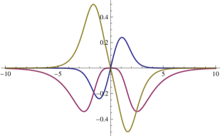
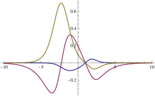
Figure 12: Components of the Jacobi fields (7.6) for $\sigma=0.7$, $\epsilon_{1}=\epsilon_{2}=\epsilon_{3}=0$, and $\gamma=\bar{\gamma}=0$ (left), $\gamma=1$, $\bar{\gamma}=2$ (right).

The existence of a conjugate point establishes, according with Morse theory, that these kink solutions are not stable under small perturbations. In fact, the Morse index theorem states that the number of negative eigenvalues of the second order fluctuation operator around a given orbit is equal to the number of conjugate points crossed by the orbit [20]. The reason is that the spectrum of the Schrödinger operator has in this case an eigenfunction with as many nodes as the Morse index, the Jacobi field, whereas the ground state has no nodes. The Jacobi fields of the $NTK$ orbits cross one conjugate point, their Morse index is one, and the $NTK$ kinks are unstable.

Finally, it is possible to extend these results to the $N=3$ case, where two Jacobi fields appear, and the instability of the generic $TK$ family is showed. The procedure is the same, but the extension of the expressions is considerably bigger, thus we will not include this calculation here.

Acknowledgements

We are very grateful to J. Mateos Guilarte for informative and illuminating conversations on several issues concerning this work. We also thank the Spanish Ministerio de Educación y Ciencia and Junta de Castilla y León for partial support under grants FIS2006-09417 and GR224.

References

- [1]
- [2] Alonso Izquierdo A., González León M.A., Mateos Guilarte J., Kinks in a nonlinear massive sigma model, Phys. Rev. Lett. 101 (2008), 131602, 4 pages, arXiv:0808.3052.
- [3] Alonso Izquierdo A., González León M.A., Mateos Guilarte J., BPS and non-BPS kinks in a massive nonlinear -sigma model, Phys. Rev. D 79 (2009), 125003, 16 pages, arXiv:0903.0593.
- [4] Alonso Izquierdo A., González León M.A., Mateos Guilarte J., Senosiain M.J., On the semiclassical mass of -kinks, J. Phys. A: Math. Theor. 42 (2009), 385403, 18 pages, arXiv:0906.1258.
- [5] Gell-Mann M., Lévy M., The axial vector current in beta decay, Nuovo Cimento (10) 16 (1960), 705–726.
- [6] Brézin E., Zinn-Justin J., Le Guillou J.C., Renormalization of the nonlinear -model in 2+ dimensions, Phys. Rev. D 14 (1976), 2615–2621.
- [7] Woodford S.R., Barashenkov I.V., Stability of the Bloch wall via the Bogomolnyi decomposition in elliptic coordinates, J. Phys. A: Math. Teor. 41 (2008), 185203, 11 pages, arXiv:0803.2299.
-
[8]
Barashenkov I.V., Woodford S.R., Zemlyanaya E.V.,
Interactions of parametrically driven dark solitons. I. Néel–Néel and Bloch–Bloch interactions,
Phys. Rev. E 75 (2007), 026604, 18 pages,
nlin.SI/0612059.
Barashenkov I.V., Woodford S.R., Interactions of parametrically driven dark solitons. II. Néel–Bloch interactions, Phys. Rev. E 75 (2007), 026605, 14 pages, nlin.SI/0701005. - [9] Barashenkov I.V., Woodford S.R., Zemlyanaya E.V., Parametrically driven dark solitons, Phys. Rev. Lett. 90 (2003), 054103, 4 pages, nlin.SI/0212052.
- [10] Rajaraman R., Solitons and instantons. An introduction to solitons and instantons in quantum field theory, North-Holland Publishing Co., Amsterdam, 1982.
- [11] Alonso Izquierdo A., González León M.A., Mateos Guilarte J., Kink manifolds in (1+1)-dimensional scalar field theory, J. Phys. A: Math. Gen. 31 (1998), 209–229.
- [12] Alonso Izquierdo A., Mateos Guilarte J., Generalized MSTB models: structure and kink varietes, Phys. D 237 (2008), 3263–3291, arXiv:0802.0153.
- [13] Alonso Izquierdo A., González León M.A., Mateos Guilarte J., Kinks from dynamical systems: domain walls in a deformed linear sigma model, Nonlinearity 13 (2000), 1137–1169, hep-th/0003224.
- [14] Neumann C., De problemate quodam mechanico, quod ad primam integralium ultraelipticorum classem revocatur, J. Reine Angew. Math. 56 (1859), 46–63.
- [15] Moser J., Various aspects of integrable Hamiltonian systems, in Dynamical Systems (C.I.M.E. Summer School, Bressanone, 1978), Progr. Math., Vol. 8, Birkhäuser, Boston, 1980, 233–289.
- [16] Dubrovin B.A., Theta functions and nonlinear equations, Uspekhi Mat. Nauk 36 (1981), no. 2, 11–80.
- [17] Alonso Izquierdo A., González León M.A., Mateos Guilarte J., Stability of kink defects in a deformed linear sigma model, Nonlinearity 15 (2002), 1097–1125, math-ph/0204041.
- [18] Bogomolnyi E.B., The stability of classical solutions, Soviet J. Nuclear Phys. 24 (1976), 449–454.
- [19] Mumford D., Tata lectures on theta. II. Jacobian theta functions and differential equations, Progr. Math., Vol. 43, Birkhäuser, Boston, 1984.
- [20] Ito H., Tasaki H., Stability theory for nonlinear Klein–Gordon kinks and the Morse’s index theorem, Phys. Lett. A 113 (1985), 179–182.