Abstract

We have derived the unitarity bounds in the high energy limit for the minimal $B-L$ extension of the Standard Model by analysing the full class of Higgs and would-be Goldstone boson two-to-two scatterings at tree level. Moreover, we have investigated how these limits could vary at some lower critical value of the energy.

1 Introduction

Despite there is no experimental evidence of a Higgs boson, the Higgs mechanism is still largely considered as one of the preferred means of generating masses for all known (and possibly new) particles. For this reason, in the last three decades or so, a global effort has been done to profile the massive scalar boson(s) coming from Electro-Weak Symmetry Breaking (EWSB), both within the Standard Model (SM) and Beyond it (BSM).

In the SM there is just one Higgs doublet consisting of four real scalar fields, three of which, after spontaneous EWSB, turn out to be absorbed in the longitudinal polarisation component of each of the three weak gauge bosons, $W^{\pm}$ and $Z$, whilst the fourth one gives the physical Higgs state $H$. Even if there are models in which the mass of this particle is predicted, this is not generally possible within the SM framework (or any of its non-supersymmetrical extensions encompassing the Higgs mechanism), hence several theoretical methods have been developed to constrain its value (see [1], [2], [3]). For example, to stay with the SM, the pioneeristic work of [2] showed that, when $m_{H}$ is greater than a critical value $\simeq 1$ TeV (known as unitarity bound), the elastic spherical wave describing the scattering of the longitudinally polarised vector bosons at very high energy ($\sqrt{s}\rightarrow\infty$) violates unitarity at tree level and the theory stops to be valid from a perturbative point of view. Moreover, it has also been shown that, well before the infinite energy limit, the unitarity bound is violated already at some lower energy critical value $\sqrt{s_{c}}>m_{H}$. The strongest such a bound, that we can call “critical energy unitarity bound”, is $m_{H}\simeq 1.09$ TeV (again, for the SM, for example see [4]).

In the past, several efforts have been devoted to applying these methodologies to a variety of models in order to extract any possible information on their allowed parameter space. In particular, it has been already applied to scenarios with extended scalar sectors yet with same gauge structure as the SM, like those with additional singlets (for example, see [5]), doublets (for example, see [4] and [6] for non-Supersymmetric scenarios and [7] for Supersymmetric ones), triplets (for example, see [8]). It has also been shown that this approach is successful with respect to $U(1)$ gauge group extensions of the SM (for example, for the case of $E_{6}$ superstring-inspired minimal $U(1)$ extensions, see [9]).

In the present work, we want to apply these two methods to the minimal $B-L$ gauged extension of the SM [10]. The latter, with respect to the SM, consists of a further $U(1)_{B-L}$ gauge group, three right-handed neutrinos and an additional Higgs boson generated through the $U(1)_{B-L}$ symmetry breaking, responsible for giving mass to an additional $Z^{\prime}$ gauge boson. It is important to note that in this model the ${B-L}$ breaking can take place at the TeV scale, i.e., far below that of any Grand Unified Theory (GUT). (This $B-L$ scenario therefore has interesting phenomenological implications at present and future colliders [11].) Hence, if one wants to study the aforementioned unitarity constraints in this framework, the presence of two Higgs fields and four massive vector bosons should be taken into account. As we will show in the remainder of the paper, the main difference with respect to analogous treatments of minimal $U(1)$ extensions of the SM (as done in [9]) is that we are not considering here the possibility of fixing any of the free parameters of the model by exploiting GUT arguments.

This work is organised as follows: in the next section we describe the model in its relevant (to this analysis) parts, in the following one we show the theoretical methods adopted to constrain the Higgs masses, in section 4 we present our numerical results, then we conclude in section 5.

2 The scalar sector of the minimal $B-L$ model

The model under study is the so-called “pure” or “minimal” $B-L$ model (see [11] for conventions and references) since it has vanishing mixing between the two $U(1)_{Y}$ and $U(1)_{B-L}$ gauge groups. In the rest of this paper we refer to this model simply as the “$B-L$ model”. In this model the classical gauge invariant Lagrangian, obeying the $SU(3)_{C}\times SU(2)_{L}\times U(1)_{Y}\times U(1)_{B-L}$ gauge symmetry, can be decomposed as:

$$\mathscr{L}=\mathscr{L}_{YM}+\mathscr{L}_{s}+\mathscr{L}_{f}+\mathscr{L}_{Y}\,,$$ (1)

where $\mathscr{L}_{YM}$, $\mathscr{L}_{s}$, $\mathscr{L}_{f}$ and $\mathscr{L}_{Y}$ are the Yang-Mills, scalar, fermionic and Yukawa sectors, respectively. Since it has been proven that perturbative unitarity violation at high energy occurs only in vector and Higgs bosons elastic scatterings, our interest is focused on the vector boson and scalar sectors. In particular, as intimated in the previous section, it is well known that in such processes the amplitude of the spherical partial wave can exceed the unit value.

In this connection then, we want to stress again that this model has an extended gauge sector, with an additional electrically neutral weak gauge boson, $Z^{\prime}$, with respect to the SM. To realise the Higgs mechanism (breaking the $SU(2)_{L}\times U(1)_{Y}$ as well as $U(1)_{B-L}$ symmetries) we must in turn introduce at least a complex Higgs field $\chi$, which is a singlet state.

Now, following the BRS invariance (see [12]), we know that the amplitude for emission or absorption of a ‘scalarly’ polarised gauge boson becomes equal to the amplitude for emission or absorption of the related Goldstone boson, and, in the high energy limit ($s\gg m^{2}_{W^{\pm},Z,Z^{\prime}}$) the amplitude involving the (physical) longitudinal polarisation of gauge bosons approaches the one involving the (unphysical) scalar one (Equivalence Theorem, see [13]).

Since it is the spherical partial wave of the former that gives rise to unitarity violation, the analysis of the perturbative unitarity of two-to-two particle scattering in the gauge sector can be performed, in the high energy limit, by exploiting the Goldstone sector.

Moreover, while evaluating scalar bosons scattering amplitudes, we have explicitely verified by numerical computation that, in the search for the Higgs mass limits, the contribution that arises from the intermediate vector boson exchange is not relevant. Hence, in the high energy limit, we can substitute the vector boson and Higgs boson sectors with the related (would-be) Goldstone and Higgs boson sectors.

For the purpose of this work, we will therefore focus on the scalar interacting Lagrangian of the Higgs and would-be Goldstone sectors (in the Feynman gauge), i.e., the scalar Lagrangian neglecting the gauge couplings in the covariant derivative.

The scalar Lagrangian is:

$$\mathscr{L}_{s}=\left(D^{\mu}H\right)^{\dagger}D_{\mu}H+\left(D^{\mu}\chi\right)^{\dagger}D_{\mu}\chi-V(H,\chi)\,,$$ (2)

with the scalar potential given by

$$V(H,\chi)=-m^{2}H^{\dagger}H-\mu^{2}\mid\chi\mid^{2}+\lambda_{1}(H^{\dagger}H)^{2}+\lambda_{2}\mid\chi\mid^{4}+\lambda_{3}H^{\dagger}H\mid\chi\mid^{2}\,,$$ (3)

where $H$ and $\chi$ are the complex scalar Higgs doublet and singlet fields, respectively:

$$H=\frac{1}{\sqrt{2}}\left(\begin{array}[]{c}-i(w^{1}-iw^{2})\\ v+(h+iz)\end{array}\right),\qquad\chi=\frac{1}{\sqrt{2}}(x+(h^{\prime}+iz^{\prime})),$$ (6)

where $w^{\pm}=w^{1}\mp iw^{2}$, $z$ and $z^{\prime}$ are would-be Goldstone bosons of $W^{\pm}$, $Z$ and $Z^{\prime}$, respectively. Even for a minimal $B-L$ model we have a generic mixing between $h$ and $h^{\prime}$. Considering $h_{1}$ and $h_{2}$ (with $m_{h_{1}}<m_{h_{2}}$) as the two Higgs mass eigenstates corresponding to the two mass eigenvalues

$$m^{2}_{h_{1}} = \lambda_{1}v^{2}+\lambda_{2}x^{2}-\sqrt{(\lambda_{2}x^{2}-\lambda_{1}v^{2})^{2}+(\lambda_{3}xv)^{2}},$$ (7)

$$m^{2}_{h_{2}} = \lambda_{1}v^{2}+\lambda_{2}x^{2}+\sqrt{(\lambda_{2}x^{2}-\lambda_{1}v^{2})^{2}+(\lambda_{3}xv)^{2}},$$ (8)

we can write the matrix that realises the Higgs mixing as

$$\left(\begin{array}[]{c}h_{1}\\ h_{2}\end{array}\right)=\left(\begin{array}[]{cc}\cos{\alpha}&-\sin{\alpha}\\ \sin{\alpha}&\cos{\alpha}\end{array}\right)\left(\begin{array}[]{c}h\\ h^{\prime}\end{array}\right),$$ (15)

with $\alpha\in[-\frac{\pi}{2},\frac{\pi}{2}]$ (since the system is invariant under $\alpha\rightarrow\alpha+\pi$ we halve the domain of the orthogonal transformation), and

$$\sin{(2\alpha)} = \frac{\lambda_{3}xv}{\sqrt{(\lambda_{2}x^{2}-\lambda_{1}v^{2})^{2}+(\lambda_{3}xv)^{2}}},$$ (16)

$$\cos{(2\alpha)} = \frac{\lambda_{2}x^{2}-\lambda_{1}v^{2}}{\sqrt{(\lambda_{2}x^{2}-\lambda_{1}v^{2})^{2}+(\lambda_{3}xv)^{2}}}.$$ (17)

In terms of physical parameters we can write

$$v=\frac{m_{W}\sin{\theta_{W}}}{\sqrt{\pi\alpha}}=\frac{m_{W}}{\sqrt{\pi\alpha_{W}}},\qquad x=\frac{m_{Z^{\prime}}}{2g^{\prime}_{1}},$$ (18)

where $v(x)$ is the Higgs doublet(singlet) Vacuum Expectation Value (VEV).

From this, we can extrapolate the relation between $\lambda$’s and Higgs masses and mixing angle:

$$\lambda_{1} = \frac{m_{h_{1}}^{2}}{2v^{2}}+\frac{\left(m_{h_{2}}^{2}-m_{h_{1}}^{2}\right)}{2v^{2}}\sin^{2}{\alpha}=\frac{m_{h_{1}}^{2}}{2v^{2}}\cos^{2}{\alpha}+\frac{m_{h_{2}}^{2}}{2v^{2}}\sin^{2}{\alpha}$$

$$\lambda_{2} = \frac{m_{h_{1}}^{2}}{2x^{2}}+\frac{\left(m_{h_{2}}^{2}-m_{h_{1}}^{2}\right)}{2x^{2}}\cos^{2}{\alpha}=\frac{m_{h_{1}}^{2}}{2x^{2}}\sin^{2}{\alpha}+\frac{m_{h_{2}}^{2}}{2x^{2}}\cos^{2}{\alpha}$$

$$\lambda_{3} = \frac{\left(m_{h_{2}}^{2}-m_{h_{1}}^{2}\right)}{2vx}\sin{(2\alpha)}$$ (19)

hence, we can calculate the explicit form of the interactions (i.e., the Feynman rules) of the Lagrangian in terms of mass eigenstates and couplings. We have listed the complete set of these functions in appendix A.

3 Theoretical bounds on the Higgs boson masses in the $B-L$ model

In this section we want to explain in some detail the techniques that we have used in order to obtain the aforementioned unitarity bounds. The salient idea stems from the connection between perturbative unitarity of a theory and a consequent upper bound on the Higgs mass, or masses (in BSM scenarios), firstly described in detail by [2].

The well known result is that by evaluating the tree-level scattering amplitude of longitudinally polarised vector bosons one finds that the latter grows with the energy of the process, eventually violating unitarity, unless one includes some other (model dependent) interactions.

As already intimated, we also know that the equivalence theorem allows one to compute the amplitude of any process with external longitudinal vector bosons $V_{L}$ ($V=W^{\pm},Z,Z^{\prime}$), in the limit $m^{2}_{V}\ll s$, by substituting each one of them with the related Goldstone bosons $v=w^{\pm},z,z^{\prime}$ and its general validity is proven (see [13]); schematically, if we consider a process with four longitudinal vector bosons: $M(V_{L}V_{L}\rightarrow V_{L}V_{L})=M(vv\rightarrow vv)+O(m_{V}^{2}/s)$.

We have also verified that, in the high energy limit, the intermediate vector boson exchange does not play a fundamental role in the Higgs boson(s) limits search, hence we simplify our approach by employing a theory of interacting would-be Goldstone bosons $v=w^{\pm},z,z^{\prime}$ described by the scalar Lagrangian in eq. (2).

We therefore studied the unitarity constraints in the $B-L$ model by calculating tree-level amplitudes for all two-to-two processes involving the full set of possible (pseudo)scalar fields (the most relevant subset is given by table 1).

Given a tree-level scattering amplitude between two spin-$0$ particles, $M(s,\theta)$, where $\theta$ is the scattering (polar) angle, we know that the partial wave amplitude with angular momentum $J$ is given by

$$a_{J}=\frac{1}{32\pi}\int_{-1}^{1}d(\cos{\theta})P_{J}(\cos{\theta})M(s,\theta),$$ (20)

where $P_{J}$ are Legendre polynomials. It has been proven (see [14]) that, in order to preserve unitarity, each partial wave must be bounded by the condition

$$|\textrm{Re}(a_{J}(s))|\leq\frac{1}{2}.$$ (21)

It turns out that only $J=0$ (corresponding to the spherical partial wave contribution) leads to some bound, so we will not discuss the higher partial waves any further.

We have verified that, in the high energy limit, only the four-point vertexes (related to the four-point functions of the interacting potential, eqs. (34)–(36) of App. A) contribute to the $J=0$ partial wave amplitudes, and this is consistent with many other works that exploit the same methodology (for example, see [4], [6] and [7]).

Hence, we will present the main results of our study focusing only on the relevant subset of all spherical partial wave amplitudes that is shown in table 1. Here, we should notice that, as one can conclude from direct computation, in the high energy limit the contributions in table 1 ticked with $\sim$ are just a double counting of the channels ticked with $\surd$ or combinations of them.

	$zz$	$w^{+}w^{-}$	$z^{\prime}z^{\prime}$	$h_{1}h_{1}$	$h_{1}h_{2}$	$h_{2}h_{2}$
$zz$	$\surd$	$\surd$	$\surd$	$\surd$	$\surd$	$\surd$
$w^{+}w^{-}$	$\sim$	$\surd$	$\sim$	$\sim$	$\sim$	$\sim$
$z^{\prime}z^{\prime}$	$\sim$	$\sim$	$\surd$	$\surd$	$\surd$	$\surd$
$h_{1}h_{1}$	$\sim$	$\sim$	$\sim$	$\surd$	$\surd$	$\surd$
$h_{1}h_{2}$	$\sim$	$\sim$	$\sim$	$\sim$	$\surd$	$\surd$
$h_{2}h_{2}$	$\sim$	$\sim$	$\sim$	$\sim$	$\sim$	$\surd$

Table 1: The most relevant subset of two-to-two scattering processes in the minimal $B-L$ model in the Higgs and would-be Goldstone boson sectors. The rows(columns) refer to the initial(final) state (or vice versa). The symbol $\sim$ refers to processes that can be computed by appropriate rearrangements of those symbolised by $\surd$.

Moreover, we have explicitely verified by numerical computation that the main contributions come from the so-called scattering eigenchannels, i.e., the diagonal elements of the “matrix” in table 1. In particular, for our choice of method, only the $zz\to zz$ and $z^{\prime}z^{\prime}\to z^{\prime}z^{\prime}$, and to a somewhat lesser extent also $h_{1}h_{1}\to h_{1}h_{1}$ and $h_{2}h_{2}\to h_{2}h_{2}$, play a relevant role. For completeness, we list here all the $a_{0}$’s, eigenchannel by eigenchannel:

$$a_{0}(zz\rightarrow zz) = \frac{3\alpha_{W}}{32m_{W}^{2}}\left[m_{h_{1}}^{2}+m_{h_{2}}^{2}+\left(m_{h_{1}}^{2}-m_{h_{2}}^{2}\right)\cos{(2\alpha)}\right],$$ (22)

$$a_{0}(w^{+}w^{-}\rightarrow w^{+}w^{-}) = \frac{\alpha_{W}}{16m_{W}^{2}}\left[m_{h_{1}}^{2}+m_{h_{2}}^{2}+\left(m_{h_{1}}^{2}-m_{h_{2}}^{2}\right)\cos{(2\alpha)}\right],$$ (23)

$$a_{0}(z^{\prime}z^{\prime}\rightarrow z^{\prime}z^{\prime}) = \frac{3}{32\pi x^{2}}\left[m_{h_{1}}^{2}+m_{h_{2}}^{2}-\left(m_{h_{1}}^{2}-m_{h_{2}}^{2}\right)\cos{(2\alpha)}\right],$$ (24)

$$a_{0}(h_{1}h_{1}\rightarrow h_{1}h_{1}) = \frac{3\alpha_{W}}{32m_{W}^{2}}\left[m_{h_{1}}^{2}+m_{h_{2}}^{2}+\left(m_{h_{1}}^{2}-m_{h_{2}}^{2}\right)\cos{(2\alpha)}\right]\cos^{4}{\alpha}$$ (25)

$$- \frac{3\sqrt{\alpha_{W}}}{64m_{W}\sqrt{\pi}x}\left(m_{h_{1}}^{2}-m_{h_{2}}^{2}\right)\sin^{3}{(2\alpha)}$$

$$+ \frac{3}{16\pi x^{2}}\left[m_{h_{1}}^{2}-\left(m_{h_{1}}^{2}-m_{h_{2}}^{2}\right)\cos^{2}{\alpha}\right]\sin^{4}{\alpha},$$

$$a_{0}(h_{1}h_{2}\rightarrow h_{1}h_{2}) = \frac{\sqrt{\alpha_{W}}}{256m_{W}\sqrt{\pi}x}\left(m_{h_{1}}^{2}-m_{h_{2}}^{2}\right)(\sin{(2\alpha)}-3\sin{(6\alpha)})$$ (26)

$$+ \frac{3}{64\pi x^{2}}\left[m_{h_{1}}^{2}-\left(m_{h_{1}}^{2}-m_{h_{2}}^{2}\right)\cos^{2}{\alpha}\right]\sin^{2}{(2\alpha)}$$

$$+ \frac{3\alpha_{W}}{64m_{W}^{2}}\left[m_{h_{1}}^{2}-\left(m_{h_{1}}^{2}-m_{h_{2}}^{2}\right)\sin^{2}{\alpha}\right]\sin^{2}{(2\alpha)},$$

$$a_{0}(h_{2}h_{2}\rightarrow h_{2}h_{2}) = \frac{3}{16\pi x^{2}}\left[m_{h_{1}}^{2}-\left(m_{h_{1}}^{2}-m_{h_{2}}^{2}\right)\cos^{2}{\alpha}\right]\cos^{4}{\alpha}$$ (27)

$$- \frac{3\sqrt{\alpha_{W}}}{64m_{W}\sqrt{\pi}x}\left(m_{h_{1}}^{2}-m_{h_{2}}^{2}\right)\sin^{3}{(2\alpha)}$$

$$+ \frac{3\alpha_{W}}{16m_{W}^{2}}\left[m_{h_{1}}^{2}-\left(m_{h_{1}}^{2}-m_{h_{2}}^{2}\right)\sin^{2}{\alpha}\right]\sin^{4}{\alpha}.$$

We remark upon the fact that in the high energy limit, $\sqrt{s}\rightarrow\infty$, only the $a_{0}$ partial wave amplitude (i.e., the four-point function as one can conclude by direct comparison between eqs. (22)–(27) and eqs. (34)–(36) in App. A) does not vanish, instead it approaches a value depending only on $m_{h_{1}}$, $m_{h_{2}}$ and $\alpha$. Therefore, by applying the condition in eq. (21), we can obtain several different (correlated) constraints on the Higgs masses and mixing angle, i.e., we can find the $m_{h_{1}}$-$m_{h_{2}}$-$\alpha$ subspace in which the perturbative unitarity of the theory is valid up to any energy scale.

Let us now come to another bound, often referred to as “triviality bound” in some literature, but which is essentially a unitarity bound obtained at some finite energy. Another question one could ask is how much the above constraint would be relaxed if the analysis were done not in the infinite energy limit $\sqrt{s}\rightarrow\infty$ but rather at a critical energy value $\sqrt{s}\rightarrow\sqrt{s}_{c}$ for which the bound on the Higgs masses is the most relaxed possible.

To this end, we developed a simple technique that is based on the following idea: after fixing the Higgs mixing angle, we perform the integral in eq. (20) on the $m_{h_{1}}$-$m_{h_{2}}$ subspace defined by eq. (21) applied to the $a_{0}$’s by varying the value of $\sqrt{s}$ in order to find the critical energy $\sqrt{s}_{c}$ for which the result is maximal.

For illustration, let us consider the channels $zz\rightarrow zz$ and $z^{\prime}z^{\prime}\rightarrow z^{\prime}z^{\prime}$ as we have already mentioned that they are the most relevant ones. We evaluated that their spherical partial waves, in the limit $m_{Z}\ll m_{h_{1}},m_{h_{2}}$ and $m_{Z^{\prime}}\ll m_{h_{1}},m_{h_{2}}$ respectively, are

$$a_{0}(zz\rightarrow zz;s) = a_{0}(zz\rightarrow zz;s\rightarrow\infty)$$ (28)

$$+ \frac{\alpha_{W}m_{h_{1}}^{2}}{16m_{W}^{2}}\left(\frac{m_{h_{1}}^{2}}{s-m_{h_{1}}^{2}}-\frac{2m_{h_{1}}^{2}}{s}\ln{\left[\frac{\left(m_{h_{1}}^{2}+s\right)}{m_{h_{1}}^{2}}\right]}\right)\cos^{2}{\alpha}$$

$$+ \frac{\alpha_{W}m_{h_{2}}^{2}}{16m_{W}^{2}}\left(\frac{m_{h_{2}}^{2}}{s-m_{h_{2}}^{2}}-\frac{2m_{h_{2}}^{2}}{s}\ln{\left[\frac{\left(m_{h_{2}}^{2}+s\right)}{m_{h_{2}}^{2}}\right]}\right)\sin^{2}{\alpha},$$

$$a_{0}(z^{\prime}z^{\prime}\rightarrow z^{\prime}z^{\prime};s) = a_{0}(z^{\prime}z^{\prime}\rightarrow z^{\prime}z^{\prime};s\rightarrow\infty)$$ (29)

$$+ \frac{m_{h_{1}}^{2}}{16\pi x^{2}}\left(\frac{m_{h_{1}}^{2}}{s-m_{h_{1}}^{2}}-\frac{2m_{h_{1}}^{2}}{s}\ln{\left[\frac{\left(m_{h_{1}}^{2}+s\right)}{m_{h_{1}}^{2}}\right]}\right)\sin^{2}{\alpha}$$

$$+ \frac{m_{h_{2}}^{2}}{16\pi x^{2}}\left(\frac{m_{h_{2}}^{2}}{s-m_{h_{2}}^{2}}-\frac{2m_{h_{2}}^{2}}{s}\ln{\left[\frac{\left(m_{h_{2}}^{2}+s\right)}{m_{h_{2}}^{2}}\right]}\right)\cos^{2}{\alpha}.$$

We can integrate these functions then at fixed angle $\alpha$ in order to establish which is the value of $\sqrt{s}$ that maximises the integral (and thus the relative allowed configuration space), in turn producing the most relaxed upper bound on the Higgs masses $m_{h_{1}}$ and $m_{h_{2}}$ at fixed $\alpha$.

In the next section we will explore the potential of these two criteria, i.e., unitarity at either infinite or finite energy, in constraining the Higgs parameter space, in terms of the mixing angle between the two physical Higgs fields and their masses.

4 Results

In the following subsections we will show that the most relevant scattering channels for the unitarity analysis are pure-$z$ and pure $z^{\prime}$-bosons scatterings. As one can see from eqs. (22)-(24), and eqs. (28)-(29), the limit coming from these two channels is unaffected by the transformation $\alpha\rightarrow-\alpha$, hence it is not restrictive to consider the half domain $\alpha\in[0,\frac{\pi}{2}]$ only. Furthermore, we remind the reader that we are still not allowing the inversion of the Higgs mass eigenvalues, i.e., we still require $m_{h_{1}}<m_{h_{2}}$.

4.1 Unitarity bounds

In this subsection we study the space of the parameters $\alpha$, $m_{h_{1}}$ and $m_{h_{2}}$, once it has been specified by the unitarity condition applied to the spherical partial wave scattering amplitudes listed in the previous section in the very high energy limit.

For a start, let us mention that, after performing a complete numerical analysis, we discovered that there only two eigenchannels that play any role in this study and these are the $zz\rightarrow zz$ and $z^{\prime}z^{\prime}\rightarrow z^{\prime}z^{\prime}$ scattering processes. Nevertheless, we must also point out the fact that, for particular choices of $\alpha$, the Higgs scattering channels (chiefly, $h_{1}h_{1}\to h_{1}h_{1}$ and $h_{2}h_{2}\to h_{2}h_{2}$) partially bound the Higgs mass space just as the gauge boson scattering channels. For example, if we choose $\alpha\rightarrow 0$, then we have that the upper bound on the $m_{h_{1}}$ mass from $h_{1}h_{1}\rightarrow h_{1}h_{1}$ is exactly the same as the one that we can extract from the evaluation of $zz\rightarrow zz$, while if we choose $\alpha\rightarrow\pi/2$, then we have that the upper bound on the $m_{h_{2}}$ mass from $h_{2}h_{2}\rightarrow h_{2}h_{2}$ is exactly the same as the one that we can extract from the evaluation of $z^{\prime}z^{\prime}\rightarrow z^{\prime}z^{\prime}$.

We want to start our analysis in the $m_{h_{1}}$-$m_{h_{2}}$ subspace, hence we “slice” the $3$-dimensional parameter space we are dealing with by keeping the Higgs mixing angle fixed.

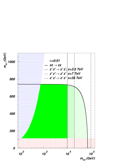
(a)

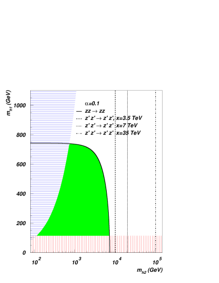
(b)

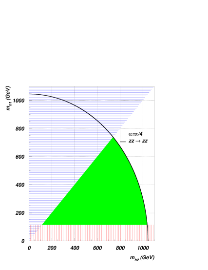
(c)

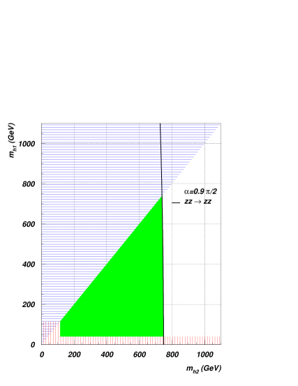
(d)

Figure 1: Higgs bosons mass limits in the $B-L$ model coming from the unitarity condition $|\textrm{Re}(a_{0})|\leq\frac{1}{2}$ applied to the $zz\rightarrow zz$ and $z^{\prime}z^{\prime}\rightarrow z^{\prime}z^{\prime}$ scatterings for several values of $x$, for $\alpha=0.01$ (1a), $\alpha=0.1$ (1b), $\alpha=\pi/4$ (1c) and $\alpha=0.9\ \pi/2$ (1d). The (blue) horizontal shadowed region corresponds to the unphysical configuration $m_{h_{1}}>m_{h_{2}}$. The (red) vertical shadowed region is excluded by the LEP experiments.

By applying the unitarity constraint to the spherical partial waves listed in the previous section, one discovers that for a mixing angle $\alpha$ such that

$${\rm{arctan}}\left(\frac{m_{W}}{x\sqrt{\pi\alpha_{W}}}\right)\leq\alpha\leq\frac{\pi}{2}$$ (30)

the allowed parameter space is completely defined by the $zz\rightarrow zz$ eigenchannel.

We will call “high-mixing domain” the parameter space defined by a choice of the mixing angle in this range, while the “low-mixing domain” is the complementary one. For example, since $x\geq 3.5$ TeV following the LEP analyses [15], if we choose $x$ to be exactly $3.5$ TeV, then we say that the high-mixing domain, in this particular case, is the one for $0.073\leq\alpha\leq\frac{\pi}{2}$ (and, conversely, the low-mixing one is in the interval $0\leq\alpha<0.073$).

We can appreciate how the size of the Higgs mixing affects the limits on the Higgs masses by looking at figure 1, in which we plot the allowed space for the latter, limitedly to the two eigenchannels $zz\rightarrow zz$ and $z^{\prime}z^{\prime}\rightarrow z^{\prime}z^{\prime}$, for four different values of $\alpha$ and three of $x$ (the latter affects only the limit coming from the $z^{\prime}z^{\prime}\to z^{\prime}z^{\prime}$ scattering).

We see that in both cases, as expected, the light Higgs mass upper bound does not exceed the SM one (which is $\simeq 700$ GeV, according to [14]), and it runs to the experimental lower limit from LEP (according to [16]) as the heavy Higgs mass increases. This is because the two Higgses ‘cooperate’ in the unitarisation of the eigenchannels so that, if one Higgs mass tends to grow, the other one must become lighter and lighter in order to keep the scattering matrix elements unitarised.

While we are in the high-mixing domain, as in figure 1b-1c-1d (where $\alpha=0.1$, $\alpha=\frac{\pi}{4}$, $\alpha=0.9\ \frac{\pi}{2}$, respectively), the allowed region coming from the $zz\to zz$ scattering is completely included in the $z^{\prime}z^{\prime}\to z^{\prime}z^{\prime}$ allowed area, and the highest value allowed for the heavy Higgs mass only depends on the mixing angle via

$${\rm{Max}}(m_{h_{2}})=2\sqrt{\frac{2}{3}}\ \frac{m_{W}}{\sqrt{\alpha_{W}}\sin{\alpha}}.$$ (31)

When we move to figure 1a (where $\alpha=0.01$, low-mixing domain) we are able to appreciate some interplay between the two scattering processes. In fact, in this case, while the $zz\to zz$ scattering eigenchannel allows the existence of a heavy Higgs of more than $10$ TeV, the $z^{\prime}z^{\prime}\to z^{\prime}z^{\prime}$ scattering channel strongly limits the allowed mass region, with a “cut-off” on the heavy Higgs mass almost insensible to the light Higgs mass (and the value of the mixing angle, since we are in the low-mixing domain), that is

$${\rm{Max}}(m_{h_{2}})\simeq 2\sqrt{\frac{2\pi}{3}}x,$$ (32)

which is in agreement (under different theoretical assumptions though) with the result in [9]; from a graphical point of view, in figure 1a the (green) hollow area represents the allowed configuration space at $x=3.5$ TeV, while at $x=10$ TeV the allowed portion of the $m_{h_{1}}$-$m_{h_{2}}$ subspace increases until the (green) double-lines shadowed region, finally the constraint relaxes to the (green) single line shadowed region when $x=35$ TeV.

This interplay effect arising (somewhat unintuitively) for Higgs low-mixing is due to the fact that the consequent decoupling between the two Higgs states requires the light(heavy) Higgs state to independently keep the scattering matrix elements of the $z^{(^{\prime})}z^{(^{\prime})}\rightarrow z^{(^{\prime})}z^{(^{\prime})}$ process unitary, thus realising two separate constraints: the first on the light (SM-like) Higgs mass due to the $zz\rightarrow zz$ unitarisation and the second on the heavy ($B-L$ like) Higgs mass due to the $z^{\prime}z^{\prime}\rightarrow z^{\prime}z^{\prime}$ unitarisation.

To summarise, given a value of the singlet Higgs VEV $x$ (compatible with experiment), the upper bound on the light Higgs boson mass varies between the SM limit and the experimental lower limit from LEP as long as the upper bound for the heavy Higgs mass increases. Moreover, when $\alpha$ assumes a value included in the high-mixing domain, the strongest bound comes from the unitarisation of the $z$-boson scattering, whilst in the low-mixing domain the bound on the heavy Higgs mass coming from that channel relaxes and the unitarisation induced by the $z^{\prime}$-boson scattering becomes so important to also impose a cut-off (which depends linearly on $x$) on the heavy Higgs mass.

This is a very important result, because it allows us to conclude that, whichever the Higgs mixing angle, both Higgs boson masses of the $B-L$ model are bounded from above. As examples of typical values for the heavy Higgs mass, in table 2, we show some upper bounds that universally apply (i.e., no matter what the mixing angle is) once the singlet Higgs VEV is given.

$x$ (TeV)	Max$(m_{h_{2}})$ (TeV)
$3.5$	$\simeq 10$
$7$	$\simeq 20$
$10$	$\simeq 30$
$20$	$\simeq 60$
$35$	$\simeq 100$

Table 2: Universal upper bound on the heavy Higgs mass, $m_{h_{2}}$, in the $B-L$ model as a function of the singlet Higgs VEV, $x$.

Before we move on, it is also worth re-emphasising that, if the Higgs mixing angle is such that we are in the high-mixing case, the upper bound on the heavy Higgs boson mass coming from $z$-boson scattering is more stringent than the one coming from $z^{\prime}$-boson scattering and it is totally independent from the chosen singlet Higgs VEV.

Nowadays, it is important to refer in our analysis to the possibility of a Higgs boson discovery either at Tevatron or Large Hadron Collider (LHC). Thus, if we suppose that a light or heavy Higgs mass $m_{h_{1}}$ has been already measured by an experiment it is interesting to study the $\alpha$-$m_{h_{2}}$ parameter space, to see whether an hitherto unassigned Higgs state can be consistent with a minimal $B-L$ scenario.

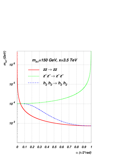
(a)

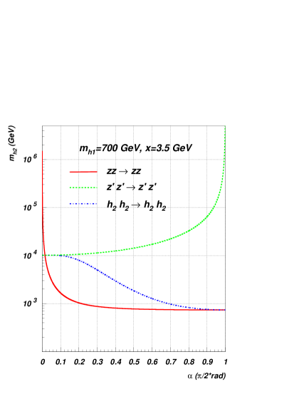
(b)

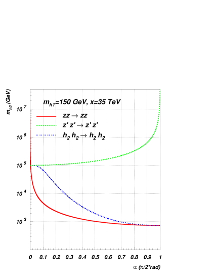
(c)

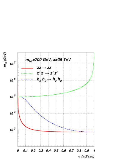
(d)

Figure 2: Heavy Higgs boson mass limits plotted against the mixing angle $\alpha$ in the minimal $B-L$ model. We have applied the unitarity condition $|\textrm{Re}(a_{0})|\leq\frac{1}{2}$ on $zz\rightarrow zz$ (red straight line), $z^{\prime}z^{\prime}\rightarrow z^{\prime}z^{\prime}$ (green dashed line) and $h_{2}h_{2}\rightarrow h_{2}h_{2}$ (blue dashed-dotted line) scatterings. This has been plotted for two fixed values of the light Higgs boson mass ($m_{h_{1}}=150$ GeV (2a, 2c) and $m_{h_{1}}=700$ GeV (2b, 2d)) and of the singlet Higgs VEV ($x=m_{Z^{\prime}}/(2g^{\prime}_{1})=3.5$ TeV (2a, 2b) and $x=m_{Z^{\prime}}/(2g^{\prime}_{1})=35$ TeV (2c, 2d)).

To this end, in figure 2 we fix $m_{h_{1}}$ and $x$ at two extreme configurations: we take $m_{h_{1}}=150$ GeV as minimum value (conservatively, taking a figure that is allowed by the experimental lower bound established by LEP for a SM Higgs boson) and $m_{h_{1}}=700$ GeV as maximum value (close to the maximum allowed by unitarity constraints, as we saw before). Then, we take $x=3.5$ TeV as minimum value (that is, the lower limit established by LEP data for the existence of a $Z^{\prime}$ of ${B-L}$ origin) and $m_{h_{1}}=35$ TeV as maximum value (that is, one order of magnitude bigger than the smallest VEV allowed by experiment).

Even in this case we can separate the $2$-dimensional subspace in a low-mixing region and a high-mixing region, as before. We can identify the first(second) as the one in which the upper bound is established by unitarisation through the $z^{\prime}$($z$)-boson scattering. The value of the mixing angle that separates the two regions in this case is given by

$$\alpha={\rm arccos}\sqrt{\frac{\left(3m_{h_{1}}^{2}-8\pi x^{2}\right)\alpha_{W}}{6m_{h_{1}}^{2}\alpha_{W}-8\pi x^{2}\alpha_{W}-8m_{W}^{2}}}.$$ (33)

Once the light Higgs boson mass is fixed, we can see how the heavy Higgs boson mass is bounded from above through the value defined by eq. (32) through the $z^{\prime}z^{\prime}\rightarrow z^{\prime}z^{\prime}$ channel, and this occurs in the low-mixing region. In particular, we can notice how the $z^{\prime}$-constraining function reaches a plateau and overlaps with the $h_{2}h_{2}\rightarrow h_{2}h_{2}$ eigenchannel bound. Moreover, if we pay attention to the high-mixing region, we see that, if $m_{h_{1}}$ is fixed to some low value, then the bound on the heavy Higgs mass relaxes much more as the mixing gets smaller and smaller with respect to the the situation in which $m_{h_{1}}$ is large, where the unitarisation is shared almost equally by $m_{h_{2}}$ and $m_{h_{1}}$.

4.2 Unitarity bounds at finite energy

So far what we did was to impose the unitarity bound at the infinite energy scale ($\sqrt{s}\rightarrow\infty$). Now we can ask how this bound could change if we choose to evaluate the same limit at some finite value of $\sqrt{s}$ in order to understand if there are new configurations in the $3$-dimensional parameter space that could invalidate our previous discussion. For this, we study how the spherical partial wave amplitude is modified by changing the parameter $\sqrt{s}$, in order to understand if the unitarity bounds loosen somewhat.

We want to refer this kind of analysis to the $m_{h_{1}}$-$m_{h_{2}}$ subspace (at fixed $\alpha$) because it is simpler to isolate the case in which the most stringent bound comes from the $zz\rightarrow zz$ eigenchannel only (imposing the condition in eq. (21) to the function defined by eq. (28)). In fact, we have already proven that in the high energy limit, even for a small mixing angle, say $\alpha=0.1$, we can limit our analysis to this one eigenchannel only and plot the integrated configuration space in function of $\sqrt{s}$. We will eventually demonstrate that this assumption is not spoiled at any finite energy scale. We remind the reader that, in order to avoid irrelevant complications, in eq. (28) we assumed that $m^{2}_{h_{1}},m^{2}_{h_{2}}\gg m^{2}_{Z}$. For this, in this subsection we take $m^{2}_{h_{1}},m^{2}_{h_{2}}\simeq 10m^{2}_{Z}$.

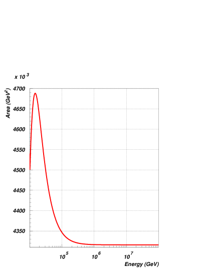
(a)

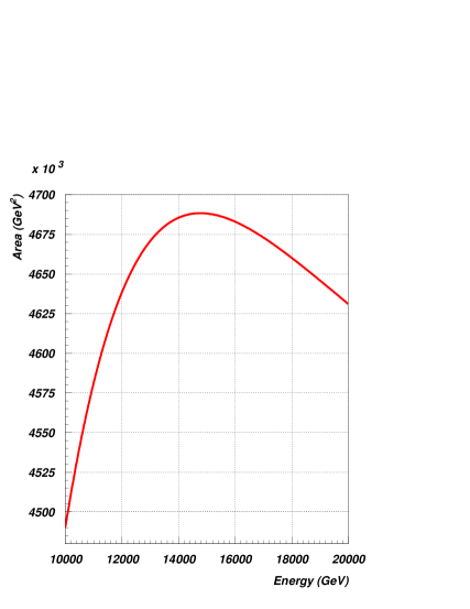
(b)

Figure 3: Integrated area of the two Higgs mass space allowed by the unitarity condition $|\textrm{Re}(a_{0})|\leq\frac{1}{2}$ applied to the scattering channel $zz\rightarrow zz$ plotted against the centre-of-mass energy of the process at fixed value of the mixing angle, $\alpha=0.1$.

As we see from figure 3, the plotted function has a local maximum, after which it tends to the asymptotic value established by the infinite energy limit. At the peak (corresponding to the critical energy $\sqrt{s}_{c}\simeq 14.7$ TeV), the allowed configuration space at fixed angle $\alpha=0.1$ is maximised. In short, by comparing the allowed space in the infinite energy limit ($A_{U}$) and the one in the critical configuration ($A_{C}$) we see that $A_{C}\simeq 1.09A_{U}$, i.e., a mere $9\%$ difference in configuration space.

Figure 4: Higgs bosons mass limits in the $B-L$ model coming from the unitarity condition $|\textrm{Re}(a_{0})|\leq\frac{1}{2}$ applied to $zz\rightarrow zz$ scattering in the high energy limit ($\sqrt{s}\rightarrow\infty$, black line) and in the critical energy limit ($\sqrt{s}\rightarrow\sqrt{s_{c}}$, green hollow area) for a fixed value of the mixing angle ($\alpha=0.1$). They have been plotted for the local maximum of the integrated area, corresponding to the critical energy $\sqrt{s}_{c}\simeq 14.7$ TeV. The (blue) horizontal shadowed region corresponds to the unphysical configurations with $m_{h_{1}}>m_{h_{2}}$. The (violet) vertical shadowed region is excluded by the assumption $m^{2}_{h_{1}},m^{2}_{h_{2}}>10m^{2}_{Z}$.

Finally, in figure 4, we want to show how the infinite energy limit relaxes in the critical energy case. Here, in essence, it emerges the fact that, generally, if we choose a finite critical energy $\sqrt{s}_{c}$ instead of the infinite energy limit and we look at the new bounds, we cannot gain more than just a few percent differences in the allowed mass space. In practise then, we can conclude that, if we choose a small mixing angle, there is no significant change in the quantitative analysis of the $m_{h_{1}}$-$m_{h_{2}}$ space with respect to the limits obtained in the infinite energy limit. (Although not illustrated here, we verified that we reach the same conclusions if we allow for large Higgs mixing instead.)

5 Conclusions

In summary, we have presented a full theoretical analysis on unitarity bounds in the Higgs sector of the minimal $B-L$ model. The scope of this endeavour was to clarify the role of the two Higgs bosons in the unitarisation of vector and scalar bosons scattering amplitudes, that we know it must hold at any energy scale.

Using the equivalence theorem, we have evaluated the spherical partial wave amplitude of all possible two-to-two scatterings in the scalar Lagrangian at an infinite energy, identifying the $zz\rightarrow zz$ and $z^{\prime}z^{\prime}\rightarrow z^{\prime}z^{\prime}$ processes as the most relevant scattering channels for this analysis ($z^{(^{\prime})}$ is the would-be Goldstone boson of the $Z^{(^{\prime})}$ vector boson).

Then, we have shown that these two channels impose an upper bound on the two Higgs masses: the light one cannot exceed the SM bound while the limit on the heavy one is established by the singlet Higgs VEV, whose value is presently constrained by LEP and could shortly be extracted by experiment following a possible discovery of a $Z^{\prime}$.

We also studied how the discovery of a light Higgs boson at either Tevatron or LHC could impact on the heavy Higgs mass bounds in the $B-L$ model and we discovered that the lighter the $h_{1}$ mass the more loose is the bound on $m_{h_{2}}$, except in the low-mixing region ($\alpha\rightarrow 0$) of the Higgs parameter space, in which the knowledge of the $x$ VEV is again fundamental.

Furthermore, we studied not only the infinite energy limit, but also some lower energy critical configuration in which the Higgs mass bounds become the most loose possible, and we discovered that in general there are small (and not relevant) differences between the limits obtained in the two cases, which amount to a few percent at most.

In conclusion, in the minimal $B-L$ framework, we expect that a TeV machine (like Tevatron, LHC or a future Linear Collider) should produce evidence of at least a light Higgs boson. The interesting possibility appearing in the $B-L$ model is that the companion heavy Higgs mass is bound to be within the reach of the machine, with the actual maximum value been dictated by the VEV $x$, i.e., the ratio between the $Z^{\prime}$ mass and its coupling, both extractable by experiment.

Appendix A Interaction potential of the scalar Lagrangian

In this appendix, we rewrite the interaction part of eq. (3) in terms of mass eigenstates, separating four-point and three-point functions and classifying them by the nature of the involved fields.

The part of the interacting potential that contains four-point functions involving only would-be Goldstone bosons is:

$$V_{4,g}=$$ (34)

$$- \frac{\pi\alpha_{W}\left(m_{h_{1}}^{2}\cos^{2}{\alpha}+m_{h_{2}}^{2}\sin^{2}{\alpha}\right)}{8m_{W}^{2}}(w^{+}w^{-}+z^{2})^{2}$$

$$- \frac{(g^{\prime}_{1})^{2}\left(m_{h_{1}}^{2}\sin^{2}{\alpha}+m_{h_{2}}^{2}\cos^{2}{\alpha}\right)}{2m_{Z^{\prime}}^{2}}(z^{\prime})^{4}$$

$$- \frac{\sqrt{\pi\alpha_{W}}g^{\prime}_{1}\left(m_{h_{2}}^{2}-m_{h_{1}}^{2}\right)\sin{(2\alpha)}}{4m_{W}m_{Z^{\prime}}}(w^{+}w^{-}+z^{2})(z^{\prime})^{2}.$$

The part of the interacting potential that contains four-point functions involving both would-be Goldstone and Higgs bosons is:

$$V_{4,hg}=$$ (35)

$$- \frac{\sqrt{\pi\alpha_{W}}\cos{\alpha}}{4m_{W}^{2}m_{Z^{\prime}}}\big{[}2g^{\prime}_{1}\left(m_{h_{2}}^{2}-m_{h_{1}}^{2}\right)m_{W}\sin^{3}{\alpha}$$

$$+ \sqrt{\pi\alpha_{W}}\left(m_{h_{1}}^{2}\cos^{2}{\alpha}+m_{h_{2}}^{2}\sin^{2}{\alpha}\right)m_{Z^{\prime}}\cos{\alpha}\big{]}h^{2}_{1}(w^{+}w^{-}+z^{2})$$

$$- \frac{\sqrt{\pi\alpha_{W}}\sin{\alpha}}{4m_{W}^{2}m_{Z^{\prime}}}\big{[}2g^{\prime}_{1}\left(m_{h_{2}}^{2}-m_{h_{1}}^{2}\right)m_{W}\cos^{3}{\alpha}$$

$$+ \sqrt{\pi\alpha_{W}}\left(m_{h_{1}}^{2}\cos^{2}{\alpha}+m_{h_{2}}^{2}\sin^{2}{\alpha}\right)m_{Z^{\prime}}\sin{\alpha}\big{]}h^{2}_{2}(w^{+}w^{-}+z^{2})$$

$$- \frac{\sqrt{\pi\alpha_{W}}\sin{(2\alpha)}}{4m_{W}^{2}m_{Z^{\prime}}}\big{[}g^{\prime}_{1}\left(m_{h_{2}}^{2}-m_{h_{1}}^{2}\right)m_{W}\sin{(2\alpha)}$$

$$+ \sqrt{\pi\alpha_{W}}\left(m_{h_{1}}^{2}\cos^{2}{\alpha}+m_{h_{2}}^{2}\sin^{2}{\alpha}\right)m_{Z^{\prime}}\big{]}h_{1}h_{2}(w^{+}w^{-}+z^{2})$$

$$- \frac{g^{\prime}_{1}\sin{\alpha}}{2m_{W}m^{2}_{Z^{\prime}}}\big{[}-\sqrt{\pi\alpha_{W}}\left(m_{h_{2}}^{2}-m_{h_{1}}^{2}\right)m_{Z^{\prime}}\cos^{3}{\alpha}$$

$$+ 2g^{\prime}_{1}\left(m_{h_{1}}^{2}\sin^{2}{\alpha}+m_{h_{2}}^{2}\cos^{2}{\alpha}\right)m_{W}\sin{\alpha}\big{]}h^{2}_{1}(z^{\prime})^{2}$$

$$- \frac{g^{\prime}_{1}\cos{\alpha}}{2m_{W}m^{2}_{Z^{\prime}}}\big{[}-\sqrt{\pi\alpha_{W}}\left(m_{h_{2}}^{2}-m_{h_{1}}^{2}\right)m_{Z^{\prime}}\sin^{3}{\alpha}$$

$$+ 2g^{\prime}_{1}\left(m_{h_{1}}^{2}\sin^{2}{\alpha}+m_{h_{2}}^{2}\cos^{2}{\alpha}\right)m_{W}\cos{\alpha}\big{]}h^{2}_{2}(z^{\prime})^{2}$$

$$- \frac{g^{\prime}_{1}\sin{(2\alpha)}}{4m_{W}m^{2}_{Z^{\prime}}}\big{[}\sqrt{\pi\alpha_{W}}\left(m_{h_{2}}^{2}-m_{h_{1}}^{2}\right)m_{Z^{\prime}}\sin{(2\alpha)}$$

$$- 4g^{\prime}_{1}\left(m_{h_{1}}^{2}\sin^{2}{\alpha}+m_{h_{2}}^{2}\cos^{2}{\alpha}\right)m_{W}\big{]}h_{1}h_{2}(z^{\prime})^{2}.$$

The part of the interacting potential that contains four-point functions involving only Higgs bosons is:

$$V_{4,h}=$$ (36)

$$- \frac{1}{16}\Bigg{[}\frac{8(g^{\prime}_{1})^{2}\left(m_{h_{1}}^{2}\sin^{2}{\alpha}+m_{h_{2}}^{2}\cos^{2}{\alpha}\right)\sin^{4}{\alpha}}{m_{Z^{\prime}}^{2}}$$

$$+ \frac{\sqrt{\pi\alpha_{W}}g^{\prime}_{1}\left(m_{h_{2}}^{2}-m_{h_{1}}^{2}\right)\sin^{3}{(2\alpha)}}{m_{W}m_{Z^{\prime}}}$$

$$+ \frac{2\pi\alpha_{W}\left(m_{h_{1}}^{2}\cos^{2}{\alpha}+m_{h_{2}}^{2}\sin^{2}{\alpha}\right)\cos^{4}{\alpha}}{m_{W}^{2}}\Bigg{]}h^{4}_{1}$$

$$- \frac{\sin{(2\alpha)}}{4m_{W}^{2}m_{Z^{\prime}}^{2}}\left(2g^{\prime}_{1}m_{W}\sin{\alpha}+\sqrt{\pi\alpha_{W}}m_{Z^{\prime}}\cos{\alpha}\right)\times$$

$$\times \Big{[}-2g^{\prime}_{1}\left(m_{h_{1}}^{2}\sin^{2}{\alpha}+m_{h_{2}}^{2}\cos^{2}{\alpha}\right)m_{W}\sin{\alpha}$$

$$+ \sqrt{\pi\alpha_{W}}\left(m_{h_{1}}^{2}\cos^{2}{\alpha}+m_{h_{2}}^{2}\sin^{2}{\alpha}\right)m_{Z^{\prime}}\cos{\alpha}\Big{]}h_{1}^{3}h_{2}$$

$$- \frac{\sin{(2\alpha)}}{16m_{W}^{2}m_{Z^{\prime}}^{2}}\Big{[}12(g^{\prime}_{1})^{2}\left(m_{h_{1}}^{2}\sin^{2}{\alpha}+m_{h_{2}}^{2}\cos^{2}{\alpha}\right)m_{W}^{2}\sin{(2\alpha)}$$

$$+ \sqrt{\pi\alpha_{W}}g^{\prime}_{1}\left(m_{h_{2}}^{2}-m_{h_{1}}^{2}\right)m_{W}m_{Z^{\prime}}(1+3\cos{(4\alpha)})$$

$$+ 3\pi\alpha_{W}\left(m_{h_{1}}^{2}\cos^{2}{\alpha}+m_{h_{2}}^{2}\sin^{2}{\alpha}\right)m_{Z^{\prime}}^{2}\sin{(2\alpha)}\Big{]}h_{1}^{2}h_{2}^{2}$$

$$- \frac{\sin{(2\alpha)}}{4m_{W}^{2}m_{Z^{\prime}}^{2}}\left(2g^{\prime}_{1}m_{W}\cos{\alpha}+\sqrt{\pi\alpha_{W}}m_{Z^{\prime}}\sin{\alpha}\right)\times$$

$$\times \Big{[}-2g^{\prime}_{1}\left(m_{h_{1}}^{2}\sin^{2}{\alpha}+m_{h_{2}}^{2}\cos^{2}{\alpha}\right)m_{W}\cos{\alpha}$$

$$+ \sqrt{\pi\alpha_{W}}\left(m_{h_{1}}^{2}\cos^{2}{\alpha}+m_{h_{2}}^{2}\sin^{2}{\alpha}\right)m_{Z^{\prime}}\sin{\alpha}\Big{]}h_{1}h_{2}^{3}$$

$$- \frac{1}{16}\Bigg{[}\frac{8(g^{\prime}_{1})^{2}\left(m_{h_{1}}^{2}\sin^{2}{\alpha}+m_{h_{2}}^{2}\cos^{2}{\alpha}\right)\cos^{4}{\alpha}}{m_{Z^{\prime}}^{2}}$$

$$+ \frac{\sqrt{\pi\alpha_{W}}g^{\prime}_{1}\left(m_{h_{2}}^{2}-m_{h_{1}}^{2}\right)\sin^{3}{(2\alpha)}}{m_{W}m_{Z^{\prime}}}$$

$$+ \frac{2\pi\alpha_{W}\left(m_{h_{1}}^{2}\cos^{2}{\alpha}+m_{h_{2}}^{2}\sin^{2}{\alpha}\right)\sin^{4}{\alpha}}{m_{W}^{2}}\Bigg{]}h^{4}_{2}.$$

The part of the interacting potential that contains three-point functions involving both would-be Goldstone and Higgs bosons is:

$$V_{3,hg}=$$ (37)

$$- \frac{\sqrt{\pi\alpha_{W}}m_{h_{1}}^{2}\cos{\alpha}}{2m_{W}}h_{1}(w^{+}w^{-}+z^{2})$$

$$- \frac{\sqrt{\pi\alpha_{W}}m_{h_{2}}^{2}\sin{\alpha}}{2m_{W}}h_{2}(w^{+}w^{-}+z^{2})$$

$$+ \frac{g^{\prime}_{1}m_{h_{1}}^{2}\sin{\alpha}}{m_{Z^{\prime}}}h_{1}(z^{\prime})^{2}-\frac{g^{\prime}_{1}m_{h_{2}}^{2}\cos{\alpha}}{m_{Z^{\prime}}}h_{2}(z^{\prime})^{2}.$$

The part of the interacting potential that contains three-point functions involving only Higgs bosons is:

$$V_{3,h}=$$ (38)

$$- \frac{m_{h_{1}}^{2}}{2}\Bigg{(}-\frac{2g^{\prime}_{1}\sin^{3}{\alpha}}{m_{Z^{\prime}}}+\frac{\sqrt{\pi\alpha_{W}}\cos^{3}{\alpha}}{m_{W}}\Bigg{)}h_{1}^{3}$$

$$- \frac{\sin{(2\alpha)}}{4m_{W}m_{Z^{\prime}}}(2m_{h_{1}}^{2}+m_{h_{2}}^{2})\Big{(}2g^{\prime}_{1}m_{W}\sin{\alpha}+\sqrt{\pi\alpha_{W}}m_{Z^{\prime}}\cos{\alpha}\Big{)}h_{1}^{2}h_{2}$$

$$- \frac{\sin{(2\alpha)}}{4m_{W}m_{Z^{\prime}}}(m_{h_{1}}^{2}+2m_{h_{2}}^{2})\Big{(}-2g^{\prime}_{1}m_{W}\cos{\alpha}+\sqrt{\pi\alpha_{W}}m_{Z^{\prime}}\sin{\alpha}\Big{)}h_{1}h_{2}^{2}$$

$$- \frac{m_{h_{2}}^{2}}{2}\Bigg{(}\frac{2g^{\prime}_{1}\cos^{3}{\alpha}}{m_{Z^{\prime}}}+\frac{\sqrt{\pi\alpha_{W}}\sin^{3}{\alpha}}{m_{W}}\Bigg{)}h_{2}^{3}.$$

References

- [1] D. A. Dicus, V. S. Mathur, Phys. Rev. D 7 (1973) 3111.
- [2] B. W. Lee, C. Quigg, H. B. Thacker, Phys. Rev. D 16 (1977) 1519.
- [3] R. Dashen, H. Neuberger, Phys. Rev. Lett. 50 (1983) 1897.
- [4] J. Maalampi, J. Sirkka, I. Vilja, Phys. Lett. B 265 (1991) 371.
- [5] G. Cynolter, E. Lendvai and G. Pocsik, Acta Phys. Polon. B 36 (2005) 827.
- [6] H. Huffel, G. Pocsik, Z. Phys. C 8 (1981) 13.
- [7] R. Casalbuoni, D. Dominici, F. Ferruglio, R. Gatto, Nucl. Phys. B 299 (1988) 117.
- [8] M. Aoki, S. Kanemura, Phys. Rev. D 77 (2008) 095009.
- [9] R. W. Robinett, Phys. Rev. D 34 (1986) 182.
- [10] K. Huitu, S. Khalil, H. Okada, S.K. Rai, Phys. Rev. Lett. 101 (2008) 181802; W. Emam, S. Khalil, Eur. Phys. J. C 522 (2007) 625.
- [11] L. Basso, A. Belyaev, S. Moretti, C. H. Shepherd-Themistocleous, Phys. Rev. D 80 (2009) 055030.
- [12] C. Becchi, A. Rouet, R. Stora, Ann. Phys. 98 (1976) 287.
- [13] M. S. Chanowitz, M. K. Gaillard, Nucl. Phys. B 261 (1985) 379.
- [14] M. Luscher, P. Weisz, Nucl. Phys. B 300 (1988) 325.
- [15] G. Cacciapaglia, C. Csaki, G. Marandella, A. Strumia, Phys. Rev. D 74 (2006) 033011.
- [16] R. Barate et al. [LEP Working Group for Higgs boson searches and ALEPH Collaboration], Phys. Lett. B 565 (2003) 61 [arXiv:hep-ex/0306033].