$H$-band thermal emission from the 19-hour period planet WASP-19b ^,

We present the first ground-based detection of thermal emission from an exoplanet in the $H$-band. Using HAWK-I on the VLT, we observed an occultation of WASP-19b by its G8V-type host star. WASP-19b is a Jupiter-mass planet with an orbital period of only 19 h, and thus, being highly irradiated, is expected to be hot. We measure an $H$-band occultation depth of $0.259^{+0.046}_{-0.044}$ %, which corresponds to an $H$-band brightness temperature of $T_{H}=2580\pm 125$ K. A cloud-free model of the planet’s atmosphere, with no redistribution of energy from day-side to night-side, under predicts the planet/star flux density ratio by a factor of two. As the stellar parameters, and thus the level of planetary irradiation, are well-constrained by measurement, it is likely that our model of the planet’s atmosphere is too simple.

1 Introduction

For a planet that is occulted by its host star, we can measure the planet’s emergent flux and thus determine its brightness temperature without spatially resolving the system (e.g., Charbonneau et al. 2005; Deming et al. 2005). From this, we can determine a planet’s albedo and the efficiency with which energy is redistributed from the day-side to the night-side of the planet (e.g., Barman et al. 2008; Alonso et al. 2009a). By measuring occultations over a range of wavelengths, we can map the planet’s spectral energy distribution (SED) and can thus infer its chemical composition (e.g., Swain et al. 2009a), investigate whether a temperature inversion exists (i.e., a stratosphere; e.g., Charbonneau et al. 2008; Knutson et al. 2008), and constrain the albedo and the day/night energy redistribution more strongly.

The Spitzer Space Telescope (Werner et al. 2004) has measured planetary thermal emission in the 3.6–24 $\mu$m range for 15 exoplanets (e.g., Deming et al. 2009; Cowan & Agol 2010; and references therein). These observations appeared to identify two classes of short-period, giant planets, those with stratospheres and those without, depending on whether there are upper-atmosphere absorbers, and hence the planet’s effective temperature (e.g., Fortney et al. 2008). Retarded cooling produced by opaque atmospheres is one possible cause of the anomalously large measured radii (compared to the predictions of simple models) of several exoplanets (e.g., Burrows et al. 2007).

For some inflated planets, such as WASP-17b (Anderson et al. 2010), tidal heating from the circularisation of an eccentric orbit seems a more likely explanation. Measuring orbital eccentricity is essential to constrain the current and past rates of tidal heating, and the timing of occultations is essential for constraining the eccentricity.

The Spitzer measurements probe only the uppermost layers of the exoplanet atmospheres studied to date because their SEDs peak in the 2–4 $\mu$m range. Observations at shorter wavelengths are needed to probe the deeper layers of the atmosphere where energy redistribution takes place (Burrows et al. 2007), and to provide greater leverage when trying to estimate the slope of the temperature structure. Giant planets with orbital periods of a day and shorter are starting to be discovered (Hebb et al. 2009; Hellier et al. 2009; Hebb et al. 2010). With SED peaks around 1 $\mu$m, measurements bluewards of Spitzer wavelengths are even more important for these planets to estimate the bolometric luminosity and thus measure the temperature, albedo, and energy redistribution efficiency.

Spitzer’s wavelength coverage is invaluably extended by ground-based facilities, which have measured occultations in the near-infrared (near-IR) detect: OGLE-TR-56b ($z^{\prime}$-band, Sing & López-Morales 2009), TrES-3b ($K$-band, de Mooij & Snellen 2009), and CoRoT-1b (2.09 $\mu$m, Gillon et al. 2009a; and $K_{s}$-band, Rogers et al. 2009). The Hubble Space Telescope has also measured occultations in the near-IR for the two exoplanets with the brightest host stars (HD 189733b, Swain et al. 2009a; and HD 209458b, Swain et al. 2009b). Both, CoRoT (Alonso et al. 2009a, 2009b; Snellen et al. 2009) and Kepler (Borucki et al. 2009) are now also measuring occultations from space in the optical.

In this paper, we present the first ground-based detection of $H$-band thermal emission from an exoplanet. Our target, WASP-19b (Hebb et al. 2010), is a Jupiter-mass planet in a 19-h orbit around a G8V-type star, and is the shortest-period exoplanet currently known.

2 Observations

We observed an occultation of WASP-19b by its $H_{\rm mag}=10.6$ host star with the cryogenic, near-IR imager HAWK-I (Pirard et al. 2004, Casali et al. 2006), mounted on Yepun of the Very Large Telescope (Paranal, Chile). HAWK-I is composed of four Hawaii-2RG chips, each measuring 2048x2048 pixels. Its pixel scale is 0.106”/pixel, providing a total field of view of 7$\aas@@fstack{\prime}$5 x 7$\aas@@fstack{\prime}$5. Observations were obtained on 2009 May 03 from 23h06 to 05h17 UT. The broadband $H$-band filter was used ($\lambda_{\rm eff}$ = 1.620 $\mu$m, FWHM = 0.289 $\mu$m). The airmass ranged from 1.09 to 2.62 during the run and the transparency conditions were good. A total of 405 exposures, each comprising 10 integrations of 1.26 s, were obtained. We used a pattern of six offsets, with the aim of producing an accurate sky map for each image from the neighbouring images. For a given offset, we kept the stars on the same pixels to minimise the effect of the small-scale spatial variations in the sensitivity of the detector chips. As the pointing was changed once early in the run, each star sampled a total of 12 detector positions. To avoid saturation of the target and reference stars, the telescope was heavily defocused, resulting in asymmetric stellar images with FWHMs of 13–28″.

In our analysis, we used only the images obtained with the $Q1$ chip, which contained WASP-19 and several reference stars. After a standard pre-reduction (dark subtraction and flat-field division), a localised smoothing was applied to each image: the count level of each pixel was compared to the median count level of the neighbouring pixels and, if the difference exceeded a threshold of 4 $\sigma$ (or 30 $\sigma$ for pixels belonging to stellar images), then the pixel’s count level was set to the median of its neighbours. At this stage, a sky map was constructed for and removed from each image using a median-filtered set of the adjacent images taken at different offsets. For each of the 12 offsets, aperture photometry was then performed using the IRAF/DAOPHOT software (Stetson, 1987). An aperture radius of 30 pixels was used. A similar flux extraction was also performed on the non-sky-subtracted images and found to provide a more reliable result. We attribute this to the incomplete removal of the large, asymmetric stellar images from the sky maps. We thus decided to use the fluxes extracted from the non-sky-subtracted images in our analysis, though we did measure the sky level in an annulus and subtract it from the stellar aperture.

After a careful choice of reference stars, differential photometry was performed and a light curve was produced for each of the 12 offsets (Fig. 1). The light curve of one offset is signifcantly poorer than the 11 others, probably because of a detector defect in the image of either WASP-19 or a reference star, and we discarded this light curve from our analysis. For each of the 11 remaining light curves, the scatter is much larger during one half-hour period. This period corresponds to the minimum of the FWHM of the stellar images and to the maximum pixel value (above 30 kADU) for the target star. The larger scatter in this portion of the light curves is therefore probably caused by a non-linearity effect, and so we discarded these data. The 276 measurements remaining (from an original 405 measurements) after rejection are shown in Fig. 1.

Each light curve varies differently with time, and we found that these variations are strongly correlated with the background amplitudes. We chose not to simply detrend the light curves for external parameters and analyse the resulting corrected light curves. To avoid underestimating the error bars of our final parameters, we included trend models in our global analysis (Sect. 3).

Figure 1: $Top$: The 405 HAWK-I measurements from the twelve pointing offsets. The light curve from each offset was given the same normalisation factor. $Bottom$: The 276 measurements remaining after the rejection of one offset and an half-hour period that exhibited a non-linearity issue. The light curves were normalised on a per-offset basis.

3 Data analysis

To place as many observational constraints as possible on the occultation parameters, we performed a global analysis of our HAWK-I occultation photometry combined with the 34 radial velocities (RVs) and the FTS $z$-band transit light curve presented in Hebb et al. (2010). In addition, the SuperWASP transit epoch reported by Hebb et al. (2010) was used to constrain the orbital period of the planet. These data were adopted as input of the adaptative Markov-Chain Monte Carlo (MCMC) algorithm presented in Gillon et al. (2009a, 2009b). This MCMC implementation uses the Metropolis-Hasting algorithm (e.g., Carlin & Louis 2008) to sample the posterior probability distribution of adjusted parameters for a given model. Our model was based on an occulting star and a transiting planet on a Keplerian orbit about their common centre of mass. We used a classical Keplerian model for the RVs obtained outside of transit (we discarded the single RV obtained during transit). To model the eclipse photometry, we used the photometric eclipse model of Mandel & Agol (2002), multiplied by a systematic effect model.

For the FTS transit, a quadratic limb-darkening law was assumed. Quadratic coefficients $u_{1}$ and $u_{2}$ were interpolated from the tables of Claret (2004) for the Sloan $z^{\prime}$-filter and for $T_{\rm eff}$ $=5500\pm 100$ K, $\log g$ $=4.5\pm 0.2$, and [Fe/H] = $0.02\pm 0.09$ (Hebb et al. 2010). We obtained $u_{1}=0.250\pm 0.015$ and $u_{2}=0.304\pm 0.008$. We allowed the quadratic coefficients $u_{1}$ and $u_{2}$ to float in our MCMC analysis, using as jump parameters the combinations $c_{1}=2\times u_{1}+u_{2}$ and $c_{2}=u_{1}-2\times u_{2}$ to minimise the correlation of the uncertainties (Holman et al. 2006). To obtain a limb-darkening solution consistent with theory, we added to our merit function the Bayesian penalty

$$BP_{\rm\textrm{ }ld}=\sum_{i=1,2}\bigg{(}\frac{c_{i}-c^{\prime}_{i}}{\sigma_{c^{\prime}_{i}}}\bigg{)}^{2}\textrm{,}$$ (1)

where $c^{\prime}_{i}$ is the initial value deduced for the coefficient $c_{i}$ and $\sigma_{c^{\prime}_{i}}$ is its error.

For each light curve, the eclipse model was multiplied by a trend model to take into account known low-frequency noise sources (instrumental and stellar). For the FTS transit light curve, we modelled this possible trend as a quadratic time-dependent polynomial. Given the small number of points in the HAWK-I light curves obtained prior to the re-pointing of the telescope, we used a simple linear time-function as a trend model for them. For the other five HAWK-I light curves, our adopted trend model was a combination of a quadratic function of time and a quadratic function of the background amplitude. As explained in Gillon et al. (2009b), the coefficients of the trend models are not jump parameters of the MCMC, but are rather determined by least squares minimisation at each step of the MCMC. We followed the procedure described in Winn et al. (2008) to check for correlated noise in the photometric time-series and to scale the error bars accordingly. For the RVs, the quadratic addition of a jitter noise of 13 m s^-1 was needed to obtain a residual $rms$ in good agreement with the mean error in the measurements.

The jump parameters in our MCMC simulation were: the planet/star area ratio $(R_{p}/R_{s})^{2}$; the $H$-band occultation depth; the transit width (from first to last contact) $T_{14}$; the modified impact parameter $b^{\prime}=a\cos{i}/R_{\ast}$ (Gillon et al. 2009a); the orbital period $P$; the time of mid-transit $T_{0}$; the two Lagrangian parameters $e\cos{\omega}$ and $e\sin{\omega}$, where $e$ is the orbital eccentricity and $\omega$ is the argument of periastron; and $K_{2}=K\sqrt{1-e^{2}/}P^{1/3}$ (Gillon et al. 2009a), where $K$ is the semi-amplitude of the radial stellar reflex velocity. We assumed a uniform prior distribution for all of these jump parameters. The merit function used in our analysis was the sum of both the $\chi^{2}$ of each time-series and the Bayesian penalty presented in Eq. 1.

At each step of the MCMC, stellar mass was determined using the stellar mass calibration relation of Torres et al. (2009), which was derived from detailed studies of detached stellar binaries. The parameters in this relation are $\log g$, $T_{\rm eff}$  and [Fe/H], though, following the method of Enoch et al. (2010), we recast it in terms of stellar density, $\rho_{*}$, instead of $\log g$. Stellar density is constrained by observation, as it depends on the shape of the transit light curve and the eccentricity of the orbit, which is constrained by the RVs and occultation timing. The values of $T_{\rm eff}$ and [Fe/H] were drawn from the distributions $N(5500,100^{2})$ K and $N(0.02,0.09^{2})$, respectively, where $N(\mu,\sigma^{2})$ is a normal distribution with mean $\mu$ and variance $\sigma^{2}$. To account for the uncertainty in the parameters of the stellar calibration law, the values of these parameters were randomly drawn at each step of the MCMC from the normal distributions presented in Torres et al. (2009).

We first perfomed a single MCMC to assess the levels of correlated noise in the photometry and jitter noise in the RVs, and to scale the measurement error bars accordingly. This MCMC consisted of $10^{5}$ steps, with the first 20 % considered as its ‘burn-in’ phase and discarded. Five new MCMCs (10⁵ steps each, with 20 % burn-in) were then performed using the scaled error bars. The good convergence and mixing of these five MCMCs was verified using the Gelman and Rubin (1992) statistic ($R$ parameter $<$ 1 %). Finally, the inferred value and error bars of each parameter were obtained from its marginalised posterior distribution. Table 1 shows the deduced values of the jump and derived parameters. The best-fit planet model is shown in Figs. 2 and 3. As can be seen in Fig. 3 and Table 1, the occultation is clearly detected, with a depth of $0.259^{+0.046}_{-0.044}$ %. The $rms$ of the HAWK-I residuals is 0.12 %, and 0.047 % after binning in intervals of 10 measurements.

To investigate the robustness of the marginal detection of a non-zero eccentricity ($e=0.016^{+0.015}_{-0.007}$), we also perfomed an MCMC with eccentricity fixed to zero. To compare the eccentric and circular models, we computed the Bayes factor (e.g., Carlin & Louis 2008), which is the ratio of the marginal likelihoods (e.g., Chib & Jeliaskov 2001) of the two models. The deduced Bayes factor of 88 indicates that the data are more consistent with the eccentric model, though not decisively so.

Parameter (unit)	Value
Fitted model parameters (jump parameters)
$R_{p}^{2}/R_{s}^{2}$	$0.01982^{+0.00050}_{-0.00049}$
$b^{\prime}=a\cos{i}/R_{\ast}$	$0.631^{+0.026}_{-0.029}$
$T_{\rm 14}$ (days)	$0.06506^{+0.00072}_{-0.00071}$
$T_{0}$ (HJD)	$2454776.91490\pm 0.00019$
$P$ (days)	$0.7888393\pm 0.0000045$
$K_{2}$ (m s-1 days1/3)	$236.9^{+5.5}_{-5.6}$
$e\cos{\omega}$	$0.0069^{+0.0024}_{-0.0027}$
$e\sin{\omega}$	$0.005\pm 0.021$
$H$-band $F_{p}/F_{\ast}$	$0.00259^{+0.00046}_{-0.00044}$
$c_{1}$†	$0.810\pm 0.030$
$c_{2}$†	$-0.357\pm 0.022$
Dependant parameters deduced from the above
$K$ ( m s-1)	$256.5\pm 6.0$
$b_{\rm transit}$	$0.628^{+0.025}_{-0.029}$
$b_{\rm occultation}$	$0.633^{+0.033}_{-0.034}$
$T_{\rm occultation}$ (HJD)	$2454777.31281^{+0.00013}_{-0.00014}$
$a$ (AU)	$0.01659^{+0.00040}_{-0.00039}$
$i$ (°)	$80.07^{+0.72}_{-0.70}$
$e$	$0.016^{+0.015}_{-0.007}$
$\omega$ (°)	$33^{+44}_{-101}$
$M_{\ast}$ ($M_{\odot}$)	$0.977^{+0.073}_{-0.067}$
$R_{\ast}$ ($R_{\odot}$)	$0.975^{+0.038}_{-0.037}$
$\rho_{*}$ ($\rho_{\odot}$)	$1.054^{+0.095}_{-0.085}$
$u_{1}$	$0.253^{+0.015}_{-0.014}$
$u_{2}$	$0.3049\pm 0.0083$
$M_{p}$ ($M_{J}$)	$1.166^{+0.064}_{-0.061}$
$R_{p}$ ($R_{J}$)	$1.338^{+0.060}_{-0.059}$
$\rho_{p}$ ($\rho_{J}$)	$0.486^{+0.059}_{+0.051}$

Table 1: WASP-19 system parameters and 1-$\sigma$ error limits. ^†Constrained parameter; see text for details.

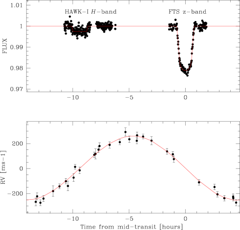
Figure 2: $Top$: Photometry of the planetary transit (FTS data, from Hebb et al. 2010) and the planetary occultation (HAWK-I data), folded on the transit ephemeris. The best-fit light curve model is superimposed. $Bottom$: Radial velocities (from Hebb et al. 2010) folded on the best-fit transit ephemeris. The best-fit RV model is superimposed.

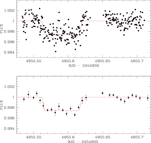
Figure 3: HAWK-I photometry corrected by the best-fit trend model for each time-series. The best-fit occultation model is superimposed. $Top$: unbinned. $Bottom$: binned every 10 measurements. Our global solution indicates a mid-occultation time of BJD=2 454 955.5905. If a circular orbit is assumed, the transit ephemeris of Table 1 predicts a time of BJD=2 454 955.5870, earlier by 0.0035 d (=5 min =0.35$\times$ a minor tic increment).

4 Discussion

We have measured a decrease in the $H$-band flux from the WASP-19 system of $0.259^{+0.046}_{-0.044}$ %, which we attribute to the occultation of day-side planetary thermal emission by the host star.

Our global solution suggests that the planet’s orbit may be non-circular, the value of $e\cos{\omega}$ being non-zero at the 2.6-$\sigma$ level; the constraint on $e\sin{\omega}$ is far weaker. The measurement of additional occultations and RVs will constrain $e\cos{\omega}$ and $e\sin{\omega}$ more strongly. A non-circular orbit may indicate that tidal heating is responsible for WASP-19b’s inflated radius (e.g., Ibgui et al. 2009).

The measured occultation depth corresponds to an $H$-band brightness temperature of $T_{H}=2580\pm 125$ K. To calculate $T_{H}$, we defined the product of the planet/star area ratio and the ratio of the bandpass-integrated planetary to stellar surface photon fluxes, corrected for transmission, to be equal to the measured occultation depth (e.g., Charbonneau et al. 2005). We assumed the planet to emit as a black body and, for the star, we used a model spectrum of a G5V star (Pickles 1998), normalised to reproduce the integrated flux of a black body with $T_{\rm eff}$ $=5500$ K (Hebb et al. 2010). The uncertainty in $T_{H}$ only takes into account the uncertainty in the measured occultation depth.

In Fig. 4, the measured $H$-band flux density ratio is compared to a model atmosphere spectrum of the planet (Barman et al. 2005), which was based on parameter values from Table 1. The model is cloud-free and adopts the nominal day-side scenario, in which the incident stellar energy remains entirely on the day-side. Given the planet’s small orbital distance from the G8V-type host star, the irradiation is quite strong ($T_{\rm eq}\approx 2400$ K, day-side only) and, in these models, it is common to see a nearly isothermal photosphere with a large temperature inversion at low pressures. In the model explored here, the inversion layers have temperatures exceeding 3000 K. Despite these high temperatures, the inversion does not extend deep enough into the photosphere to match the observed $H$-band flux; the model under predicts the flux by roughly a factor of two.

To reconcile our model’s prediction with the occultation measurement, one would need to increase the luminosity of the star by a factor of two, for example, by increasing the stellar temperature by 1000 K or increasing the host star radius by 0.4 $R_{\odot}$ (or some combination of these). These values of the stellar parameters are excluded by observations (Hebb et al. 2010; this work). The most probable explanation of the poor match to the planet flux is therefore related to the model atmosphere.

It is possible that the day-side atmosphere is much closer to pure radiative-convective equilibrium and experiences little day-side redistribution. This zero-redistribution scenario has been shown to result in a hotter substellar point and deeper occultations than the uniform day-side-only model (Barman et al. 2005). As more data are obtained, in particular at other near-IR wavelengths, we will explore a wide variety of atmospheric phenomena (e.g., clouds, depth-dependent energy redistribution, and photochemistry).

Swain et al. (2010) found a strong, unexpected 3.25-$\mu$m emission feature in the day-side spectrum of HD 189733b, which they attributed to non-local-thermodynamic-equilibrium (non-LTE) CH₄ emission. Future work should explore whether non-LTE chemistry is responsible for the unexpectedly high $H$-band flux of WASP-19b. For now, our measured $H$-band flux presents an interesting puzzle for irradiated atmospheric models.

Figure 4: Synthetic planet/star flux ratios of a cloud-free model that assumes solar abundances and no redistribution of incident stellar flux to the night-side (solid line). The effective temperature of the star was taken to be $T_{\rm eff}$ = 5500K (Hebb et al. 2010); all other parameters are taken from Table 1. The flux ratio for a black-body planet (at 2400K) is indicated by a dotted line. Solid symbols are the $H$-band integrated flux ratios; symbols without error bars correspond to the model points. The HAWK-I $H$-band filter response curve is also shown.

- (1) Alonso R., Alapini A., Aigrain S., et al., 2009a, A&A, 506, 353
- (2) Alonso R., Guillot T., Mazeh T., et al., 2009b, A&A, 501, 23
- (3) Anderson D. R., Hellier C., Gillon M., et al., 2010 ApJ, 709, 159
- (4) Barman, T. S., 2008, ApJ, 676, L61
- (5) Barman T., Hauschildt P. H., & Allard F., 2005, ApJ, 632, 1132
- (6) Borucki W. J., Koch D. G., Jenkins J., et al., 2010, Science, 325, 709
- (7) Burrows A., Hubeny I., Budaj J., & Hubbard W. B., 2007, ApJ, 661, 502
- (8) Carlin B. P., & Louis T. A., 2008, Bayesian Methods for Data Analysis, Third Edition (Chapman & Hall/CRC)
- (9) Casali M., Pirard J.-F., Kissler-Patig M., et al., 2006, SPIE, 6269, 29
- (10) Charbonneau D., Allen L. E., Megeath S. T., Torres G., & Alonso R., 2005, ApJ, 626, 523
- (11) Charbonneau D., Knutson H. A., Barman T., et al., 2008, ApJ, 686, 1341
- (12) Chib S., Jeliaskov I., 2001, JASA, 96, 270
- (13) Claret A., 2004, A&A, 428, 1001
- (14) Cowan N. B., & Agol E., 2010, ApJ (submitted), arXiv:1001.0012
- (15) de Mooij E. J. W., & Snellen I. A. G., 2009, A&A, 493, L35
- (16) Deming D., 2009, IAU Symposium, 253, 197
- (17) Deming D., Seager S., Richardson L. J., et al., 2005, Nature, 434, 740
- (18) Enoch B., Collier Cameron A., Parley N. R., Hebb L., 2010, A&A, submitted
- (19) Fortney J. J., Lodders K., Marley M. S., Freedman R. S., 2008, ApJ, 678, 1419
- (20) Gelman A., & Rubin D., 1992, Statistical Science, 7, 457
- (21) Gillon M., Lanotte A. A., Barman T., et al., 2009b, A&A, 511, 3
- (22) Gillon M., Demory B.-O., Triaud A. H. M. J., et al., 2009a, A&A, 506, 359
- (23) Hebb L., Collier-Cameron A., Loeillet B., et al., 2009, ApJ, 693. 1920
- (24) Hebb L., Collier-Cameron A., Triaud A., et al., 2010, ApJ, 708, 224
- (25) Hellier C., Anderson D. R., Cameron A. C., et al., 2009, Nature, 460, 1098
- (26) Holman M. J., Winn J. N., Latham D. W., et al., 2006, ApJ, 652, 1715
- (27) Ibgui L., Spiegel D. S., & Burrows A., 2009, ApJ (submitted), arXiv:0910.5928
- (28) Knutson H. A., Charbonneau D., Allen L. E., et al., 2008, ApJ, 673, 526
- (29) Mandel K., & Agol. E., 2002, ApJ, 5802, L171
- (30) Pickles A. J., 1998, PASP, 110, 863
- (31) Pirard J.-F., Kissler-Patig M., Moorwood A., et al., 2004, SPIE, 5492. 510
- (32) Rogers J. C., Apai D, López-Morales M., Sing D. K., Burrows A., 2009, ApJ, 707, 1707
- (33) Sing D. K., & López-Morales, M., 2009, A&A, 493, 31
- (34) Snellen I. A. G., de Mooij E. J. W., Burrows A., 2009, A&A (accepted), arXiv:0909.4080
- (35) Stetson P. B., 1987, PASP, 99, 111
- (36) Swain M. R., Deroo P., Griffith C. A., et al., 2010, Nature, 463, 637
- (37) Swain M. R., Tinetti G., Vashist G., et al., 2009b, ApJ, 704, 1616
- (38) Swain M. R., Vasisht G., Tinetti G., et al., 2009a, ApJ, 690, L114
- (39) Torres G., Andersen J., & Giménez A., 2009, A&ARv, 13
- (40) Werner M. W., Roellig T. L., & Low F. J., 2004, ApJS, 154, 1
- (41) Winn J. N., Holman M. J., Shporer A., et al., 2008, ApJ, 136, 267