Chemical and radiative transfer modeling of the ISO-LWS Fabry-Perot spectra of Orion-KL water lines

Abstract

We present chemical and radiative transfer models for the many far-IR ortho- and para-H₂O lines that were observed from the Orion-KL region in high resolution Fabry-Pérot (FP) mode by the Long Wavelength Spectrometer (LWS) on board the Infrared Space Observatory (ISO). The chemistry of the region was first studied by simulating the conditions in the different known components of Orion-KL: chemical models for a hot core, a plateau and a ridge were coupled with an accelerated $\Lambda$-iteration (ALI) radiative transfer model to predict H₂O line fluxes and profiles. Our models include the first 45 energy levels of ortho- and para-H₂O. We find that lines arising from energy levels below 560 K were best reproduced by a gas of density 3$\times$10⁵ cm^-3 at a temperature of 70-90 K, expanding at a velocity of 30 km s^-1 and with a H₂O/H₂ abundance ratio of the order of 2 - 3 $\times$ 10^-5, similar to the abundance derived by Cernicharo et al. (2006). However, the model that best reproduces the fluxes and profiles of H₂O lines arising from energy levels above 560 K has a significantly higher H₂O/H₂ abundance, 1 - 5 $\times$ 10^-4, originating from gas of similar density, in the Plateau region, that has been heated to 300 K, relaxing to 90-100 K. We conclude that the observed water lines do not originate from high temperature shocks.

1 Introduction

High velocity gas was first detected at the centre of the Orion-KL region as broad wings on ‘thermal’ molecular lines in the millimeter range and as high velocity maser features in the 22 GHz line of H₂O (Genzel et al. 1981). These high velocity motions may be caused by mass outflows from newly formed stars. Many theoretical studies of the Orion region (e.g. Draine & Roberge 1982; Chernoff et all. 1982; Neufeld & Melnick 1987) have concluded that the rich emission spectrum of thermally excited water vapor should play a significant role in cooling the gas.

The widespread distribution of water vapour around IRc2 has been probed with maps at 183 GHz (Cernicharo et al. 1990, 1994, Cernicharo & Crovisier 2005), the first time that its abundance was estimated in the different large-scale components of Orion IRc2. Harwit et al. (1998) analysed 8 water lines observed with the ISO LWS FP, concluding that these lines arise from a molecular cloud subjected to a magnetohydrodynamic C-type shock. From their modelling, they derived an H₂O to H₂ abundance ratio of 5$\times$ 10^-4. However, the interpretation of the lines observed in the $\approx$ 80^′′ LWS beam and the determination of the water abundance in the different Orion components remains a long standing problem, due to two main issues: the complexity of the dynamical and chemical processes that are taking place within the region encompassed by the LWS beam, with outflows and several different gas components, and the need for H₂O collisional rates appropriate for the temperatures prevailing in shocks.

A total of 70 water lines were detected in the ISO-LWS far-IR spectral survey of Orion-KL (Lerate et al. 2006), with typically 70 km s^-1 FWHM. The line profiles range from predominantly P-Cygni at shorter wavelengths to predominantly pure emission at longer wavelengths. At the shorter wavelengths, the heliocentric velocities of absorption components appear to be centred at $\approx$ – 15 km s^-1, consistent with the results found in the ISO Short Wavelength Spectrometer (SWS) wavelength range, shortwards of 45 $\mu$m (van Dishoeck et al. 1998; Wright et al. 2000). However, the radial velocities of the pure emission lines of H₂O peak at around +30 km s^-1, whereas the velocity of the Orion-KL quiescent gas is +9 km s^-1.

In a previous analysis of the H₂O lines observed by the ISO LWS-FP, Cernicharo et al. (2006) modeled lines from the first 30 rotational levels of ortho- an para-H₂O, concluding that the lines mainly arise from a gas flow expanding at 25-30 km s^-1, and inferred a gas temperature of approximately 80-100 K and a H₂O/H₂ abundance ratio of 2–3 $\times$ 10^-5. This derived abundance was an average over the LWS beam and they suggested that water could be locally more abundant if the emitting region included warmer components which interact with the ambient gas.

In the current work, a technique to distinguish between the different components has been applied to the final calibrated high-resolution spectra of the ortho- and para-H₂O lines from the Orion-KL region. The methodology is similar to that used to model the ISO-LWS high resolution spectra of the Orion-KL CO lines (Lerate et al. 2008). Chemical models of the physically distinct components are coupled with a non-local radiative transfer model. The description of the models is structured to follow the different components of the region: the hot core, plateau and ridge. Many references can be found for a description of the KL region components - a complete overview is given in Stahler and Palla (2004). Both models (chemical and radiative transfer) are highly configurable and have been applied to a variety of emitting regions, including molecular gas in outflows (Benedettini et al. 2006).

2 Observations and data reduction

The ISO-LWS FP observations were carried out between September 1997 and April 1998. The dataset consists of 26 individual observations making up a total of 27.9 hours of ISO LWS observing time in L03 Fabry-Perot full spectral scan mode. The dataset also includes 16 observations accumulated over 13.1 hours in L04 Fabry-Perot line scan mode and 1 observation in the lower resolution L01 grating scan mode. The instrumental field of view for all L03 observations was centred either on a position offset by 10.5^′′ from the BN object (which is at 05^h 35^m 14.12^s – 05^∘ 22^′ 22.9^′′ J2000), or on a position offset by 5.4^′′ from IRc2 (which is at 05^h 35^m 14.45^s – 05^∘ 22^′ 30.0^′′ J2000), while most of the L04 observations were centred on IRc2. The LWS beam had a diameter $\approx$ 80^′′ (Gry et al. 2003). Processing of the LWS FP data was carried out using the Offline Processing (OLP) pipeline and the LWS Interactive Analysis (LIA) package version 10. The basic calibration is fully described in the LWS handbook (Gry et al. 2003). Further processing, including dark current optimisation, de-glitching and removal of the LWS grating profile was then carried out interactively using the LWS Interactive Analysis package version 10 (LIA10; Lim et al. 2002) and the ISO Spectral Analysis Package (ISAP; Sturm 1998). A detailed description of the observations and of the data reduction process is given by Lerate et al. (2006).

3 The chemical and radiative transfer models

3.1 The Chemical Models

The chemical model used to simulate the Orion KL plateau and ridge is described by Viti et al. (2004) and is the same as used by Lerate et al. (2008) to model the Orion-KL lines observed by the ISO-LWS Fabry-Perot. The chemical network is taken from the UMIST database (Le Teuff et al. 2000). The model uses a two phase calculation in which gravitational collapse occurs in phase I, with gas-phase chemistry and sticking onto dust particles with subsequent processing (hydrogenation and conversion of a fraction of CO into methanol) also occurring. In phase II, where evaporation from grains also took place, we simulated the presence of a non-dissociative shock by an increase of temperature (from 200 to 2000K, depending on the model) at an age of $\approx$ 1000 yr, which is the dynamical timescale of the main outflow observed in the KL region (Cernicharo et al. 2006). The duration of the high temperature shock is about 100 years, representing the temperature structure of a C-shock. The gas is then allowed to cool. This temperature profile was adopted from the calculation of Bergin et al. (1998) who studied the chemistry of H₂O and O₂ in postshock gas. The treatment of the temperature increase is considered to be linear with time. The modeling allows a wide range of parameters to be varied in order to investigate a range of conditions. As with the CO modelling of Lerate et al. (2008), the main parameters that were varied in this analysis were: (i) the initial and final densities (ii) the depletion efficiency, hereafter called the freez-out parameter (iii) the cloud size (iv) the maximum gas temperature and (v) the interstellar radiation field (ISRF). Note that the H₂ column density is not a free input parameter but is calculated self-consistently as a function of size and gas density.

We based the parameter grid on descriptions of the Orion-KL components found in detailed analyses of the region (Blake et al. 1987, Genzel and Stutzki 1989, Cernicharo et al. 1994). The main parameters adopted from these references were the sizes and densities. However, we used our own analysis of the continuum emission and molecular rotational diagrams (from Lerate et al. 2006) to indicate gas temperatures. Table 1 list the main parameter sets used to compute the grid of chemical models that were used for the present H₂O modelling and for the CO modelling of Lerate et al. (2008). For completeness we also list the derived H₂ column densities for each model.

Model	Density (cm-3)	Tshock (K)	Tgas (K)	mco%	size ($\prime\prime$)	N($H_{2}$)(cm-2)
PL1	3$\times$105	200	80	40	30	4$\times$1022
PL2	3$\times$105	300	90	60	30	4$\times$1022
PL3	3$\times$105	500	90	60	30	4$\times$1022
PL4	3$\times$105	500	90	80	30	4$\times$1022
PL5	3$\times$105	1000	100	60	30	4$\times$1022
PL6	3$\times$105	1000	100	80	30	4$\times$1022
PL7	3$\times$105	2000	100	60	30	4$\times$1022
PL8	3$\times$105	2000	100	80	30	4$\times$1022
PL9	1$\times$106	300	90	60	30	2$\times$1023
PL10	1$\times$106	300	90	80	30	2$\times$1023
PL11	1$\times$106	500	90	60	30	2$\times$1023
PL12	1$\times$106	500	90	80	30	2$\times$1023
PL13	1$\times$106	1000	100	60	30	2$\times$1023
PL14	1$\times$106	1000	100	80	30	2$\times$1023
PL15	1$\times$106	2000	100	60	30	2$\times$1023
PL16	1$\times$106	2000	100	80	30	2$\times$1023
RG1	1$\times$104	no shock	70	40	15	9$\times$1020
RG2	1$\times$104	no shock	70	20	15	9$\times$1020
RG3	5$\times$104	no shock	80	40	15	5$\times$1021
RG4	5$\times$104	no shock	80	20	15	5$\times$1021

Table 1: Plateau (PL) and Ridge (RG) models and their parameters: density, maximum temperature reached by the gas in the shock simulation, gas temperature after cooling, the percentage of mantle CO (mco) given by the freeze-out parameter at the end of Stage I of the chemical model, and the approximate H₂ column density (assuming $\sim$ 1.6$\times$10²¹ cm^-2 per magnitude of visual extinction).

The chemical model used to simulate the extended gas in Orion KL is based on the same model used for the shocked gas, with the exception that no high temperature shock is included as an input. The model simulates the gas chemistry evolution of gas expanding with velocities of $\approx$ 25-30 km s^-1, which is heated up to $\approx$ 100 K on a timescale of 1000 yr, relaxing to 80 K (see Figure 1). A grid of conditions was also investigated for six extended-gas models (Table  2). Their initial parameters were based on the published literature on the Orion-KL extended gas (Tielens and Hollenbach (1985), Draine and Roberge (1982), Menten et al. (1990)).

Model	Density (cm-3)	Tgas (K)	mco%	expansion gas velocity (km s-1)
E1	3$\times$105	80	80	25
E2	3$\times$105	90	70	30
E3	5$\times$104	100	60	35
E4	3$\times$105	80	50	25
E5	3$\times$105	90	40	30
E6	5$\times$104	100	30	35

Table 2: List of main parameters modified to investigate the extended-gas chemical model of Orion KL.

3.2 The ortho-H₂O and para-H₂O radiative transfer models

As described by Lerate et al. (2008), the chemical model produces abundances that are used as inputs to the radiative transfer model SMMOL (Rawlings & Yates, 2001), along with values for the dimensions, density, dust temperature and radiation field intensity. The SMMOL code has accelerated $\Lambda$-iteration (ALI) that solves the radiative transfer problem in multi-level non-local conditions. It starts by calculating the level population assuming LTE and takes an adopted radiation field as the input continuum and then recalculates the total radiation field and level populations, repeating the process until convergence is achieved. The resulting emergent intensity distribution is then transformed to the LWS units of flux (W cm^-2 $\mu$m^-1) taking into account the different beam sizes (slightly different for each detector) and is convolved with an instrumental line profile corresponding to a 33 km s^-1 FWHM Lorentzian (Polehampton et al. 2007), in order to directly compare with the observations. The input parameters include molecular data such as the molecular mass, energy levels, radiative and collisional rates and also the dust size distribution and opacity. The parameters also include the gas and dust temperatures of the object being modelled. We estimated the dust temperature from the LWS grating observation of Orion-KL (Lerate et al. 2006), fitting a black body function of 70 K. In order to reproduce the observed continuum flux level, we adopted a radiation field equivalent to 10⁴ Habings (1 Habing unit corresponds to the integrated flux in the wavelength range from 91.2 to 111.0 nm of 1.6 $\times$ 10^-3 erg s^-1 cm^-2; Habing 1968). The adopted ortho-para ratio was 3, which was found by Barber et al. (2006) to be appropriate when T$>$50 K. The microturbulent velocity was set to 5 km s^-1 and expansion velocities from 15–40 km s^-1 were considered for the shocked gas in the Plateau models. We estimated an error of less than 30% for the fit to the continuum, being the maximum percentage deviation below the observed continuum for wavelengths up to 120 $\mu$m and the maximum percentage deviation above the observed continuum for longer wavelengths.

The o-H₂O molecular data were taken from public molecular databases (Müller et al., 2001; Schöier et al., 2005). Table 3 lists the input parameters for the radiative transfer model that were modified with respect to the CO modelling. The number of energy levels was set to 45 and the number of radiative transitions to 158. The number of collisional transitions was 990 and 10 collisional temperatures were investigated, from 20 K to 2000 K. The H₂O-H₂ collisional excitation rates were based on the (scaled) H₂O-He calculations of Green et al. (1993). Note that since the calcuations for this paper were performed new collisional rates for H₂O-H₂ have become available (Faure et al. 2007; Dubernet et al. 2009). Table 1 of Faure et al. shows that for temperatures below 300K the critical densities with helium can be factors of 2-5 greater than for rates with ortho and para hydrogen. However as our densities are at least 3 orders of magnitude below the reported critical densities, the radiative pumping terms are as important, if not more so, than the collisional pumping terms. We would therefore expect our results to be qualitatively valid within the observational errors. However one would expect the use of He as a collisional partner to be incorrect when trying to model Herschel HIFI data, because the much better angular and spectral resolution of the observations may reveal pockets of much higher density; in such cases the use of the new collisional rates for water will be necessary.

INPUT PARAMETERS	VALUE
MOLECULAR WEIGHT	18.0
NUMBER OF RADIATIVE TRANSITIONS	158
NUMBER OF COLLISION PARTNERS	1
NUMBER OF COLLISION TEMPERATURES	10
NUMBER OF COLLISIONAL TRANSITIONS	990
ISUM: THE STATISTICAL EQUILIBRIUM EQUATION FOR LEVEL ISUM IS	45
REPLACED BY THE EQUATION OF CONSERVATION OF NUMBERS
NK: NUMBER OF ENERGY LEVELS INCLUDING CONTINUUM LEVELS	45

Table 3: List of main o-H₂O and p-H₂O parameters adopted as inputs in the radiative transfer models

4 Results and Discussion

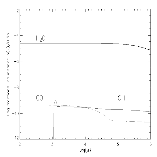
Figure 1: Time evolution H₂O, OH and CO abundances corresponding to the extended gas chemical model E2 in Table 2.

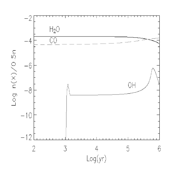
Figure 2: Time evolution of H₂O, OH and CO abundances for the PL2 chemical model (see Table 1 for a description of the main model parameters).

The H₂O line profiles and fluxes were reproduced by coupling our chemical models (see Figure 1 and Figure 2 for the final adopted chemical models) with SMMOL radiative transfer models. A large number of models were investigated, with simulations of different shock temperatures, see Table 1 and Table 2. In the models where the H₂O lines were reasonably well reproduced, an extended grid of conditions was then investigated to refine the line fits. An example of this is shown for the Extended gas model, whose investigated scenarios are summarised in Table 4. The main parameters that were modified to refine the models were the Phase II gas temperature and the freeze-out parameter, which determines the amount of water frozen onto the grains at the end of phase I of the chemical model.

Model	Density (cm-3)	Tgas (K)	gas velocity (km s-1)	mH2O (%)	H2O/H2 abundance
W1	3$\times$105	80	25	70	2.1 $\times$ 10-5
W2	3$\times$105	90	30	60	2.8 $\times$ 10-5
W3	5$\times$104	100	35	50	4.8 $\times$ 10-5
W4	3$\times$105	80	25	40	7.5 $\times$ 10-5
W5	3$\times$105	90	30	30	9.8 $\times$ 10-5
W6	5$\times$104	100	35	20	4.8 $\times$ 10-6

Table 4: List of main parameters and resulting H₂O/H₂ abundances from the chemical models adopted to investigate the extended-gas component in Orion-KL.

Wavelength	Transition	Absorbed flux	Emitted flux	Pred. absorption	Pred. emission	Line peak [1]	Line fit $\chi^{2}$
($\mu$m)		(10-17W cm-2)	(10-17W cm-2)	(10-17W cm-2)	(10-17W cm-2)	(km s-1)
49.281	p-H2O $4_{40}$ – $3_{31}$	0.71 $\pm$ 0.13		0.92		-9.2 $\pm$ 1.6	0.142
56.324	p-H2O $4_{31}$ – $3_{22}$	1.09 $\pm$ 0.11	0.59 $\pm$ 0.25	1.65		-5.1 $\pm$ 0.5, 44.9 $\pm$ 18.9	0.125
58.698	o-H2O $4_{32}$ – $3_{21}$	1.57 $\pm$ 0.13	1.80 $\pm$ 0.14	1.82	1.95	-29.9 $\pm$ 2.5, 37.3 $\pm$ 2.9	0.0368
61.808	p-H2O $4_{31}$ – $4_{04}$		0.52 $\pm$ 0.02		0.85	43.5 $\pm$ 1.7	0.0728
66.437	o-H2O $3_{30}$ – $2_{21}$	1.51 $\pm$ 0.18	1.39 $\pm$ 0.28	1.78	1.85	-22.2 $\pm$ 2.6, 40.5 $\pm$ 8.1	0.0168
71.066	p-H2O $5_{24}$ – $4_{13}$	0.15 $\pm$ 0.039	0.89 $\pm$ 0.059		1.02	-22.5 $\pm$ 5.8, 28.5 $\pm$ 1.8	0.148
71.539	p-H2O $7_{17}$ – $6_{06}$		1.39 $\pm$ 0.13		1.02	22.3 $\pm$ 2.1	0.222
75.380	o-H2O $3_{21}$ – $2_{12}$	0.88 $\pm$ 0.25	5.67 $\pm$ 0.21	1.33	4.15	-31.5 $\pm$ 8.9 , 28.5 $\pm$ 1.1	0.862
78.928	p-H2O $6_{15}$ – $5_{24}$		0.43 $\pm$ 0.11		0.35	16.5 $\pm$ 4.2	0.0551
82.030	o-H2O $6_{16}$ – $5_{05}$		2.78 $\pm$ 0.13		1.89	22.4 $\pm$ 1.1	0.361
83.283	p-H2O $6_{06}$ – $5_{15}$		1.29 $\pm$ 0.08		1.05	31.1 $\pm$ 1.8	0.181
89.988	o-H2O $3_{22}$ – $2_{11}$		2.17 $\pm$ 0.17		1.05	29.1 $\pm$ 2.3	0.542
94.703	o-H2O $4_{41}$ – $4_{32}$		0.67 $\pm$ 0.06		1.33	29.2 $\pm$ 2.7	0.181
95.626	p-H2O $5_{15}$ – $4_{04}$		1.42 $\pm$ 0.10		1.25	27.4 $\pm$ 1.3	0.184
95.883	p-H2O $4_{41}$ – $4_{32}$		0.67 $\pm$ 0.06		0.38	29.2 $\pm$ 2.7	0.121
99.492	o-H2O $5_{05}$ – $4_{14}$		5.61 $\pm$ 0.12		5.25	22.2 $\pm$ 0.5	0.448
100.913	o-H2O $5_{14}$ – $4_{23}$		3.05 $\pm$ 0.17		2.60	21.1 $\pm$ 1.2	0.366
108.073	o-H2O $2_{21}$ – $1_{10}$		3.22 $\pm$ 0.08		2.55	29.1 $\pm$ 0.7	0.418
111.626	p-H2O $5_{24}$ – $5_{15}$		0.43 $\pm$ 0.03		0.26	26.7 $\pm$ 1.7	0.068
113.944	p-H2O $5_{33}$ – $5_{24}$		1.38 $\pm$ 0.06		1.67	27.6 $\pm$ 1.3	0.207
121.719	o-H2O $4_{32}$ – $4_{23}$		2.28 $\pm$ 0.13		1.55	28.1 $\pm$ 1.6	0.342
125.354	p-H2O $4_{04}$ – $3_{13}$		2.25 $\pm$ 0.09		1.98	25.5 $\pm$ 1.1	0.202
126.713	p-H2O $3_{31}$ – $3_{22}$		0.62 $\pm$ 0.08		0.34	30.5 $\pm$ 4.1	0.093
136.494	o-H2O $3_{30}$ – $3_{21}$		0.71 $\pm$ 0.05		0.65	30.9 $\pm$ 2.3	0.113
138.527	p-H2O $3_{13}$ – $2_{02}$		2.67 $\pm$ 0.03		1.66	26.4 $\pm$ 0.3	0.293
144.517	p-H2O $4_{13}$ – $3_{22}$		1.15 $\pm$ 0.07		2.38	18.4 $\pm$ 0.2	0.287
146.919	p-H2O $4_{31}$ – $4_{22}$		1.14 $\pm$ 0.06		0.98	22.1 $\pm$ 1.1	0.216
156.193	p-H2O $3_{22}$ – $3_{13}$		1.23 $\pm$ 0.08		1.59	32.5 $\pm$ 2.2	0.258
174.626	o-H2O $3_{03}$ – $2_{12}$		2.38 $\pm$ 0.19		1.55	20.1 $\pm$ 1.6	0.333
179.527	o-H2O $2_{12}$ – $1_{01}$		2.55 $\pm$ 0.31		2.34	23.8 $\pm$ 2.9	0.204

Table 5: H₂O line fluxes observed and predicted by the modelling. [1] Observed LSR velocity. Where two values are listed, these correspond to separate emission peaks.

Line profile fits from our radiative transfer modelling are shown in Figure 3 and Figure 4, while Table 5 compares the observed and predicted line fluxes. The final column of Table 5 lists the $\chi^{2}$ values, defined as $\chi^{2}$ = $\sum_{i=1}^{N}(flux\_mod(i)-flux\_obs(i))^{2}/N(bins)$, for the comparison between the modeled (flux_mod) and observed (flux_obs) line profiles. The line profile fits are excellent for the pure emission lines, while the lines with P Cygni profiles are reasonably well reproduced.

Overall, our results can be summarised as follows:

• Lines arising from energy levels below $\approx$ 560 K are best reproduced by 70-90 K gas of density 3$\times$10⁵ cm^-3, expanding at approximately 25-30 km s^-1 (3). A graphical representation of the time evolution of H₂O, OH and CO is shown in Figure 1. corresponding to Model E2 in Table 2. Model W2 from Table 4 gives very similar results.

• Lines from higher energy levels, both ortho and para, are best reproduced by warmer gas of density 3$\times$10⁵ cm^-3, expanding at approximately 25-30 km s^-1, which is heated up to 300 K and then relaxes to 90-100 K (Figure 4). This corresponds to Model PL2 in Table 1, which also reproduced the observed CO transitions with J_up$\leq$18 (Lerate et al. 2008). Note that this is simply the best $\chi^{2}$ fit: models where the shock temperature is higher, such as PL3, also provide a good fit to the line profiles. However models where the shock temperature is of the order of 1000 K, the derived water abundance did not reproduce the line profile. We should also emphasize that the parameter that most affected the fits to the water lines was the freeze-out rate, as this directly affects the fractional abundance of water (since the higher the freeze-out rate the more oxygen is hydrogenated as water on the surfaces of the grains before evaporating). Based on the investigated models, shock temperatures in the 300-500 K range were found to produce acceptable fits to the line fluxes and profiles.

• The PL2 model which fits the higher-excitation lines shown in Figure 4 makes a negligible contribution to the lower-excitation lines shown in Figure 3, while the E2 model that fits the lower excitation lines makes a negligible contribution to the higher-excitation lines shown in Figure 4.

• The H₂O to H₂ abundance ratio is of the order of 2-3 $\times$ 10^-5 for model W2 and 1-5 $\times$ 10^-4 for model PL2.

• For the 14 para-H₂O lines that show pure emission, the ratio of the predicted to observed emission flux is found to be $0.89\pm 0.39$, while for the 10 ortho-H₂O lines that are purely in emission this ratio is also $0.89\pm 0.39$. We interpret this as observational evidence in support of the 3:1 ortho:para ratio that was adopted for the modeling.

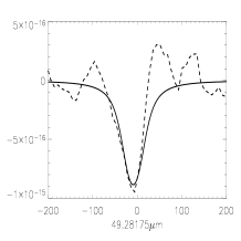
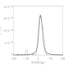
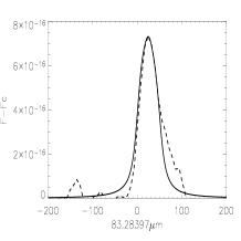
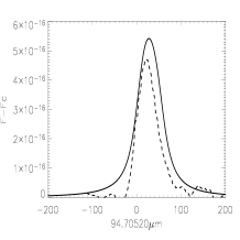
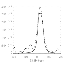
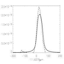
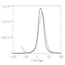
Figure 3: Predicted line profiles from the PL2 radiative transfer model (solid lines), over-plotted on the observed ortho and para-H₂O lines (dotted lines). The PL2 model corresponds to gas of density 3$\times$10⁵cm^-3, heated up to 300 K and relaxing to 90-100 K, expanding at a velocity of 30 km s^-1 (Table 1). The ordinate corresponds to the continuum-subtracted flux and the abscissa is the radial velocity in km s^-1.

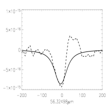
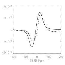
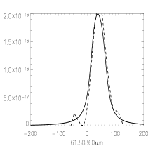
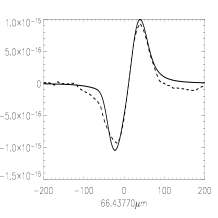
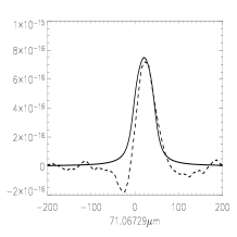
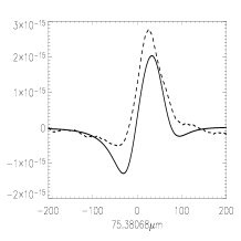
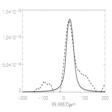
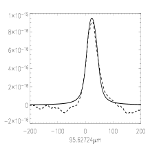
Figure 4: Predicted line profiles from the E2 radiative transfer model (solid lines) over-plotted on the observed ortho and para-H₂O lines (dotted lines). The E2 model corresponds to gas of density 3$\times$10⁵cm^-3 at 70-90 K expanding at a velocity of 30 km s^-1 (Table 2). The ordinate corresponds to the continuum-subtracted flux and the abscissa is the radial velocity in km s^-1.

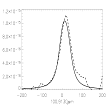
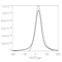
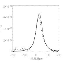
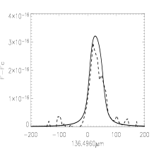
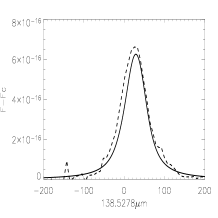
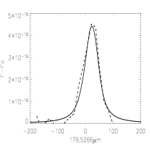
Figure 4: Continued

The results from our modeling of the observed far-IR ortho and para-H₂O lines from Orion-KL show that two different chemical models are needed to reproduce the H₂O lines in the LWS wavelength range. For lines arising from energy levels below $\approx$ 560 K, our modelling results are in agreement with the findings of Cernicharo et al. (2006); our chemical model of an expanding gas with velocity of 30 km s^-1 at 70-90 K is able to reproduce the line fluxes and line profiles of both the ortho- and para-H₂O lines, with an H₂O/H₂ abundance ratio of the order of 2-3 $\times$ 10^-5. For the water lines that exhibit P Cygni profiles, our current profile fits appear to provide an improvement when compared to the fits presented by Cernicharo et al. (2006).

However, for lines arising from higher energy levels (above 560 K) the model that best reproduces both the H₂O line fluxes and their profiles is of warmer gas which is initially heated up to $\sim$300 K and then relaxes to 90-100 K. The corresponding H₂O/H₂ abundance ratio depends on the time stage within the PL2 model but is of the order of 1-5 $\times$ 10^-4, within reach of the value of 5 $\times$ 10^-4 derived by Harwit et al. (1998) from their modelling of eight Orion-KL LWS-FP water lines. For the seven water lines in common, Harwit et al.’s mean observed/predicted line flux ratio was 1.9$\pm$1.5, versus a mean value of 1.4$\pm$0.4 from our modelling. Our PL2 model was also found to reproduce well the observed LWS-FP CO transitions having J_up$\leq$18, interpreted as arising from the Plateau region within the extended warm component emission (Lerate et al. 2008). Note, however, that, for higher-J CO lines our work shows that a higher temperature gas is needed, in agreement with other authors (e.g. Watson et al. 1985), confirming the findings of Lerate et al. (2008) that the observed molecular emission arises from multiple components that differ in density and temperature.

To conclude, we find that, taken together, Plateau region model PL2 and extended-gas region model E2 can match all of the measured far-IR water lines from Orion-KL. The main difference between the two modelled zones is that the Plateau region has warmer temperatures, with a consequent impact on the chemical evolution. As noted by Cernicharo et al. (2006), radiative pumping due to the strong IR dust continuum radiation field is sufficient to populate the higher excitation rotational water lines. The H₂O/H₂ ratio in the extended-gas region is found to be $\sim(2-3)\times 10^{-5}$, similar to the value found by Cernicharo et al. (1996) from their line modelling, but we find a significantly higher ratio, $\sim(1-5)\times 10^{-4}$, in our Plateau region models that fit the profiles and fluxes of the higher-excitation water lines.

Our present results should be taken together with those of Lerate et al. (2008), who analysed ISO LWS-FP observations of multiple rotational lines of CO and found that in order to explain the emission from all of the the CO transitions, hot cores as well as shocked regions (with temperatures ranging from 300 to 1000 K) had to be present within the ISO beam.

References

- (1) Barber, R. J., Tennyson, J., Harris, G. J., Tolchenov, R. N., 2006, MNRAS, 368, 1087
- (2) Benedettini, M, Yates, J. A., Viti, S. & Codella, C., 2006, MNRAS, 370, 229
- (3) Bergin, E. A., Neufeld, d. A., Melnick, G. J., 1998, ApJ, 499, 777
- (4) Blake, G. A., Sutton, E. C., Masson, C. R., & Phillips, T. G., 1987, ApJ, 315, 621
- (5) Cernicharo, J., Goicoechea, J. R., Daniel, F., Lerate, M. R., Barlow, M. J. et al, 2006, ApJ, 649, L33
- (6) Cernicharo, J., Gonzalez-Alfonso, E., Alcolea, J., Bachiller, R., et al., 1994, ApJ, 432, 59
- (7) Cernicharo, J.& Crovisier, J., 2005, Space Science Reviews, 119, 29
- (8) Cernicharo, J., Thum, C., Hei, H., John, D., et al., 1990, A&A, 231, 15
- (9) Chernoff, D. F., McKee, C. F., Hollenbach, D. J., 1982, ApJ, 259, 97
- (10) Dubernet, M.-L.; Daniel, F.; Grosjean, A.; Lin, C. Y., 2009, A&A, 497, 911
- (11) Draine, B. T., & Roberge, W. G., 1982, ApJ, 259, 91
- (12) Faure, A.; Crimier, N.; Ceccarelli, C.; Valiron, P.; Wiesenfeld, L.; Dubernet, M. L., 2007, A&A, 472, 1029
- (13) Genzel, R., Reid, M. J., Moran, J. M. and Downes, 1981, ApJ, 244, 844
- (14) Genzel, R., & Stutzki, J., 1989, A&A, 27, 41
- (15) Green, S., Maluendes, S and McLean, A. D. 1993, ApJS, 85, 181
- (16) Gry, C., Swinyard, B., Harwood, A., Trams, N, et al. 2003, ISO Handbook Volume III(LWS), Version 2.1, ESA SAI-99-07
- (17) Habing, H. J., 1968, Bull. Astron. Inst. Netherlands, 19, 421
- (18) Harwit, M., Neufeld, D., Melnick, G. J., Kaufman, M. J., 1998, ApJ, 497, 105
- (19) Lerate, M. R., Barlow, M. J., Swinyard, B. M., Goicoechea, J. R., et al., 2006, MNRAS, 370, 597
- (20) Lerate, M. R., Yates, J., Viti, S., Barlow, M. J., et al., 2008, MNRAS, 387, 1660
- (21) Le Teuff, Y. H., Millar, T. J., Markwick, A. J., 2000, A&AS, 146, 157L
- (22) Lim, T. L., Hutchinson, G., Sidher, S. D, Molinari, S., et al. 2002, SPIE, 4847, 435
- (23) Neufeld, D. A., & Melnick, G. J., 1987, ApJ, 332, 266
- (24) Polehampton E. T., Baluteau, J. P., Swinyard, B. M., Goicoechea, J. R., et al., 2007, MNRAS, 377, 1122.
- (25) Rawlings, J., Yates, J., 2001, MNRAS, 326, 1423
- (26) Stahler, S. W., & Palla, F., ‘The Formation of Stars’, 2004, Wiley-VCH
- (27) Sturm, E., Bauer, O.H., Lutz, D., et al. 1998, ASP 145, 161
- (28) Tielens, A. G. M. & Hollenbach, D., 1985, ApJ, 291, 722
- (29) van Dishoeck, E. F. , Wright, C. M., Cernicharo, J., Gonzalez-Alfonso, E., et al., 1998, ApJ, 502, 173
- (30) Viti, S., Codella, C., Benedettini, M. & Bachiller, R., 2004, MNRAS, 350, 1029
- (31) Viti, S., Collings, M. P., Dever, J. W., McCoustra, R. S., et al., 2004, MNRAS, 354, 1141
- (32) Viti, S. & Williams, D., 1999, MNRAS, 305, 755
- (33) Watson, D. M.; Genzel, R.; Townes, C. H.; Storey, J. W. V., 1985, ApJ, 298, 316
- (34) Wright, C. M., van Dishoeck, E. F., Black, J. H., Feuchtgruber, et al., 2000, A&A, 358,689