Monopole metrics and the orbifold
Yamabe problem

Abstract.

We consider the self-dual conformal classes on $n\#\mathbb{CP}^{2}$ discovered by LeBrun. These depend upon a choice of $n$ points in hyperbolic $3$-space, called monopole points. We investigate the limiting behavior of various constant scalar curvature metrics in these conformal classes as the points approach each other, or as the points tend to the boundary of hyperbolic space. There is a close connection to the orbifold Yamabe problem, which we show is not always solvable (in contrast to the case of compact manifolds). In particular, we show that there is no constant scalar curvature orbifold metric in the conformal class of a conformally compactified non-flat hyperkähler ALE space in dimension four.

1. Introduction

There is an interesting history regarding the existence of self-dual metrics on $n\#\mathbb{CP}^{2}$ beginning with work of Yat-Sun Poon [Po86]. Using techniques from twistor theory, Poon proved the existence of a $1$-parameter family of self-dual conformal classes on $\mathbb{CP}^{2}\#\mathbb{CP}^{2}$ and that any such conformal class with positive scalar curvature must be in this family. Examples for larger $n$ were found by Donaldson-Friedman [DF89] and Floer [Flo91] using gluing methods. In 1991, Claude LeBrun [LeB91] produced explicit examples with ${\rm{U}}(1)$-symmetry on $n\#\mathbb{CP}^{2}$, using a hyperbolic ansatz inspired by the Gibbons-Hawking ansatz [GH78]. LeBrun’s construction depends on the choice of $n$ points in hyperbolic 3-space $\mathcal{H}^{3}$. For $n=2$, the only invariant of the configuration is the distance between the monopole points, and LeBrun conformal classes are the same as the $1$-parameter family found by Poon.

1.1. Limits of LeBrun metrics

The first question we address in this paper: is there a nice compactification of the moduli space of LeBrun metrics on $n\#\mathbb{CP}^{2}$? In general, as the monopole points limit towards each other, or if the points approach the boundary of hyperbolic space, some degeneration will occur. We emphasize that the LeBrun construction produces conformal classes on $n\#\mathbb{CP}^{2}$. To discuss convergence in the Cheeger-Gromov sense, one needs to choose a conformal factor. Of course, the limit will strongly depend on the particular choice of conformal metrics. Some degenerations were already described in [LeB91] and [DF89], but these examples depended on a somewhat arbitrary choice of conformal factor.

The solution of the Yamabe problem provides one with a very natural metric in these conformal classes. However, the abstract existence theorem does not tell one what the actual minimizer looks like in any particular case, and other methods are needed to understand the geometry of minimizers. The main point of this paper is to describe the limiting behavior of the Yamabe minimizers in these conformal classes as they degenerate. In general, Yamabe minimizers are not necessarily unique; an example of non-uniqueness is given Theorem 1.1. We also examine the existence and limiting behavior of various non-minimizing constant scalar curvature metrics. Given a subgroup of the conformal automorphism group, Hebey-Vaugon have shown there is a minimizer of the Yamabe functional when restricted to the class of invariant functions (the equivariant Yamabe problem), and these automorphisms will act as isometries on the minimizer [Heb96]. Of course, a symmetric Yamabe minimizer can have higher energy than a Yamabe minimizer, and an example of this is seen in Theorem 1.1.

If $G\subset{\rm{SO}}(4)$ is a finite subgroup acting freely on $S^{3}$, then we let $G$ act on $S^{4}\subset\mathbb{R}^{5}$ acting as rotations around the $x_{5}$-axis. The quotient $S^{4}/G$ is then a orbifold, with two singular points, and the spherical metric $g_{S}$ descends to this orbifold. Near the singular points, the metric is asymptotic to a cone metric $\mathcal{C}(S^{3}/G)$, thus $S^{4}/G$ looks like a United States “football”. In the following, $G\subset{\rm{SU}}(2)$ will be a certain cyclic subgroup $\mathbb{Z}_{m}$, see (2.2) below. For a smooth Riemannian manifold $(M,g)$, the Yamabe invariant of the conformal class is denoted by $Y(M,[g])$, see Section 3. If $(M,g)$ is an orbifold, then $Y_{orb}(M,[g])$ will denote the orbifold Yamabe invariant, see Section 4.

We first discuss the special case of $n=2$. To employ the equivariant Yamabe problem, one must first understand the group of conformal automorphisms: it was proved in [HV09] that the conformal group $G$ of Poon’s metrics for $n=2$ is given by

(1.1) $$G=({\rm{U}}(1)\times{\rm{U}}(1))\ltimes D_{4},$$

where $D_{4}$ is the dihedral group of order $8$. There is the index $2$ subgroup given by

(1.2) $$K=({\rm{U}}(1)\times{\rm{U}}(1))\ltimes(\mathbb{Z}_{2}\oplus\mathbb{Z}_{2}),$$

which are exactly the lifts of hyperbolic isometries preserving the set of $2$ monopole points. In contrast, for $n>2$, any conformal automorphism of a LeBrun metric is a lift of an isometry of $\mathcal{H}^{3}$. There is an “extra” involution when $n=2$, which is not a lift of any hyperbolic isometry, see [HV09]. Let $d_{H}(\cdot,\cdot)$ denote hyperbolic distance.

Theorem 1.1.

Let $(M,g)$ be a Poon-LeBrun metric on $\mathbb{CP}^{2}\#\mathbb{CP}^{2}$ with monopole points $p_{1}$ and $p_{2}$. The Yamabe invariant satisfies the sharp estimate

(1.3) $$8\pi\sqrt{3}=Y_{orb}(S^{4}/\mathbb{Z}_{2},[g_{S}])<Y(M,[g])<Y(\mathbb{CP}^{2},[g_{FS}])=12\pi\sqrt{2}.$$

There exists a number $N$ large, such that if $d_{H}(p_{1},p_{2})>N$ then the following holds. There are two distinct Yamabe minimizers, each limiting to $g_{FS}$ on $\mathbb{CP}^{2}$ as $d_{H}(p_{1},p_{2})\rightarrow\infty$. In each case, there is one singular point of convergence at which a Burns metric bubbles off. The symmetric $K$-Yamabe minimizers limit to $(S^{4},g_{S})$ as $d_{H}(p_{1},p_{2})\rightarrow\infty$, with 2 antipodal singular points of convergence, with Burns metrics bubbling off at each of the singular points. There is a fourth constant scalar curvature metric, limiting to $\mathbb{CP}^{2}\vee\mathbb{CP}^{2}$ (the wedge of two copies of $\mathbb{CP}^{2}$ with Fubini-Study metrics, touching at a single point) as $d_{H}(p_{1},p_{2})\rightarrow\infty$. In this case, a Euclidean Schwarzschild metric with two asymptotically flat ends bubbles off.

As $d_{H}(p_{1},p_{2})\rightarrow 0$, the limit of both the Yamabe minimizers and the symmetric $K$-Yamabe minimizers is the $S^{4}/\mathbb{Z}_{2}$-football with the round metric. In both cases, at each singular point an Eguchi-Hanson metric bubbles off.

These limits are illustrated in Figure 1. An important point is that the properties of being self-dual and having constant scalar curvature form an elliptic system [TV05a]. In Tian-Viaclovsky [TV05b, TV08], it was shown that limits of such metrics may have at worst multi-fold singularities, provided that the sequence has bounded $L^{2}$-norm of curvature and does not collapse. The crucial ingredient of this theory is the upper volume growth estimate proved in [TV05a]. For other results dealing with this type of convergence in various settings, see [Aku94, Aku96, And89, And05, Ban90, CQY07, CW07, CLW08, Nak94, Tia90]. In the situation considered in this paper, the $L^{2}$-curvature bound follows from the Chern-Gauss-Bonnet formula and Hirzebruch signature theorem. The non-collapsing condition will follow from uniform positivity of the Yamabe invariant.

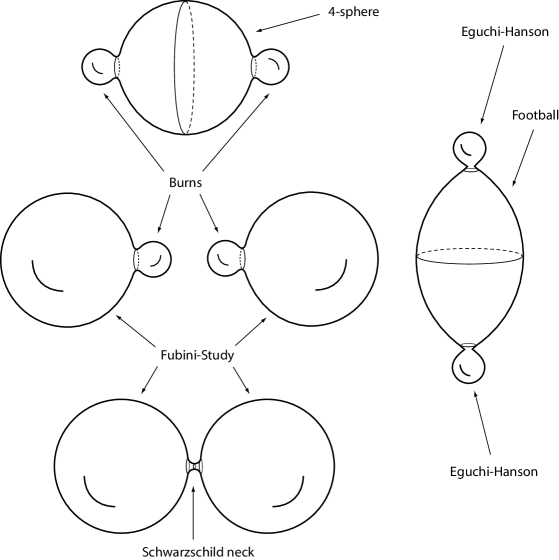
Figure 1. The 5 limiting cases described in Theorem 1.1. The left side is as $d(p_{1},p_{2})\rightarrow\infty$. The top left is the symmetric $K$-Yamabe minimizer. The middle left are the two Yamabe minimizers. The lower left is the metric obtained by Joyce gluing. The right hand side is as $d(p_{1},p_{2})\rightarrow 0$. In this case, the Yamabe minimizers and the symmetric Yamabe minimizers have the same limiting behavior. Note that in each of the above cases, to obtain $\mathbb{CP}^{2}\#\mathbb{CP}^{2}$ topologically, the attaching map for one of the factors should be orientation reversing.

As mentioned above, the LeBrun monopole construction depends upon the choice of $n$ points in hyperbolic space. An easy generalization of this construction allows one to assign integer multiplicities greater than one at the monopole points. The resulting space will have orbifold points. We call such a space a LeBrun orbifold. Next, for $n>2$, we present the following compactness theorem.

Theorem 1.2.

Let $(M,g)$ be a LeBrun self-dual conformal class on $n\#\mathbb{CP}^{2}$ with monopole points $\{p_{1},\dots,p_{n}\}$. Then

(1.4) $$Y(M,[g])\leq Y(\mathbb{CP}^{2},[g_{FS}])=12\pi\sqrt{2},$$

with strict inequality for $n\geq 2$, where $g_{FS}$ denotes the Fubini-Study metric. Next, assume that all monopole points are contained in a compact set $\mathcal{K}\subset\mathcal{H}^{3}$. Then there exists a constant $\delta_{n}$ depending only upon $n,\mathcal{K}$ such that

(1.5) $$0<\delta_{n}\leq Y(M,[g]).$$

Furthermore, any sequence of unit volume Yamabe minimizers in a sequence of LeBrun conformal classes (for fixed $n$) satisfying (1.5) has a subsequence which converges (in the Cheeger-Gromov sense) to either to (1) a compactified LeBrun orbifold metric with $1\leq k\leq n$ points or (2) the round metric on $S^{4}/\mathbb{Z}_{m}$, for some $2\leq m\leq n$. In addition, the estimate (1.5) is true for $n=2,3$ without the requirement that the points are contained in a compact set $\mathcal{K}$.

There can exist sequences of Yamabe minimizers with limiting behavior as in Case (1); this limit can occur when some of the monopole points limit to the boundary of $\mathcal{H}^{3}$, as seen in Theorem 1.1. Another example is given in Theorem 1.5 below. There also can exist sequences limiting as in Case (2), as seen in Theorem 1.1.

The estimate for the lower bound in (1.5) is not explicit, this is proved by a contradiction argument in Section 7. It would be very interesting to find a sharp constant. We conjecture that $\delta_{n}=Y_{orb}(S^{4}/\mathbb{Z}_{n},[g_{S}])$, without any requirement that the monopole points are contained in a compact set $\mathcal{K}$. For $n=2,3$, the uniform positivity of the Yamabe invariant holds for topological reasons, see Proposition 6.1.

We mention that the degeneration of the LeBrun conformal classes can also be studied using twistor theory. For this important perspective, we refer the reader to the recent paper of Nobuhiro Honda [Hon10].

1.2. The orbifold Yamabe problem

Akutagawa and Botvinnik considered the Yamabe problem on orbifolds in [AB03, AB04] in which they proved several foundational results. We will describe this in more detail in Section 4. Since the limits described above are typically orbifolds, it is no surprise that there is a close connection with the orbifold Yamabe problem. In fact, an important tool in identifying the possible limit spaces above is the following nonexistence result.

Theorem 1.3.

Let $(X_{n},g)$ be a hyperkähler ALE metric in dimension $4$, with group $G$ of order $n>1$ at infinity, and let $(\hat{X},[\hat{g}])$ denote the orbifold conformal compactification. Then $Y_{orb}(\hat{X},[\hat{g}])=Y_{orb}(S^{4}/G,[g_{S}])$, and there is no solution to the orbifold Yamabe problem on $(\hat{X},[\hat{g}])$. That is, there is no conformal metric $\tilde{g}=e^{2u}\hat{g}$ having constant scalar curvature.

This will be proved in Section 4 along with some other remarks on the orbifold Yamabe problem. The ALE metrics above, can be viewed as the Green’s function metrics $g_{p}=\Gamma_{p}^{2}\hat{g}$ of the orbifold compactification, where $\Gamma_{p}$ is the Green’s function for the conformal Laplacian of $\hat{g}$ based at the orbifold point $p$. It is interesting that these ALE spaces have zero mass and their compactifications do not admit a solution of the orbifold Yamabe problem. This shows that the orbifold Yamabe problem is more subtle than in the case of smooth manifolds.

In Section 7, we will prove another nonexistence result regarding the negative mass ALE spaces found in [LeB88].

Theorem 1.4.

If $(X,g)$ is a LeBrun negative mass ALE metric on $\mathcal{O}(-n)$ with $n>1$, then there is no symmetric solution of the orbifold Yamabe problem on $(\hat{X},\hat{g})$ invariant under $\rm{SU}(2)$.

As a consequence, the symmetric Yamabe problem on orbifolds is not always solvable either. For $n=2$, this metric is the same as the compactified Eguchi-Hanson metric, which does not admit any constant scalar curvature metric by Theorem 1.3. We do not know if there is a non-symmetric solution on these orbifolds for $n\geq 3$.

Finally, we present an existence result for the orbifold Yamabe problem, which for simplicity we state here in only the case of total multiplicity $3$ (see Corollary 4.4 for the general statement). The following theorem also shows that LeBrun orbifold metrics can in fact arise as a limit of smooth Yamabe metrics in LeBrun conformal classes, and also $k$ can be strictly less than $n$ in Case (1) of Theorem 1.2.

Theorem 1.5.

Let $(M,[g])$ be compact self-dual LeBrun orbifold corresponding to a monopole point $p_{1}$ of multiplicity $1$ and a monpole point $p_{2}$ of multiplicity $2$, with $p_{1}\neq p_{2}$. Then there exists a radius $r>0$ such that if $d_{\mathcal{H}}(p_{1},p_{2})<r$, then $(M,[g])$ admits a solution to the orbifold Yamabe problem. Furthermore, let $(M_{1},[g_{j}])$ be a self-dual LeBrun conformal class on $3\#\mathbb{CP}^{2}$ corresponding to $3$ distinct monopole points all of multiplicity one, with $p_{1}$ and $p_{2}$ fixed, and $p_{2},p_{j,3}\in B(p_{1},r)$. Then as $p_{j,3}\rightarrow p_{2}$, a subsequence of Yamabe minimizers on $(M_{1},[g_{j}])$ converges to an orbifold Yamabe metric on $(M,[g])$. There is one singular point of convergence, at which an Eguchi-Hanson metric bubbles off.

Next, let $p_{1}$ and $p_{2}$ be fixed and let $p_{j,3}$ limit to the boundary of $\mathcal{H}^{3}$ as $j\rightarrow\infty$. Then any sequence of Yamabe minimizers on $(M_{1},[g_{j}])$ has a subsequence which converges to a Yamabe minimizer in the 2-pointed smooth LeBrun conformal class $(2\#\mathbb{CP}^{2},[\hat{g}_{LB}(p_{1},p_{2})])$. There is one singular point of convergence, at which a Burns metric bubbles off.

Remark 1.6.

It is possible that $r$ could be taken to be infinite in the above theorem, but this would require a much more involved estimate of the Yamabe invariant.

1.3. Acknowledgements

The author would like to thank first and foremost, Claude LeBrun, for originally suggesting this problem and providing extremely helpful comments along the way. Peter Kronheimer and Clifford Taubes also provided very helpful suggestions early on. Nobuhiro Honda provided crucial assistance in understanding the conformal geometry of LeBrun metrics. The author held several valuable discussions with Kazuo Akutagawa regarding the orbifold Yamabe problem. Denis Auroux, Simon Donaldson, Yat-Sun Poon, and Gang Tian also gave the author some important remarks that proved to be very useful when completing this work. Finally, thanks are given to the anonymous referee whose numerous remarks and suggestions greatly improved the exposition of the paper.

2. Monopole metrics

We first recall some basic definitions.

Definition 2.1.

A Riemannian orbifold $(M^{n},g)$ is a topological space which is a smooth manifold of dimension $n$ with a smooth Riemannian metric away from finitely many singular points. At a singular point $p$, $M$ is locally diffeomorphic to a cone $\mathcal{C}$ on $S^{n-1}/G$, where $G\subset SO(n)$ is a finite subgroup acting freely on $S^{n-1}$. Furthermore, at such a singular point, the metric is locally the quotient of a smooth $G$-invariant metric on $B^{n}$ under the orbifold group $G$.

A Riemannian multi-fold $M$ is a connected space obtained from a finite collection of Riemannian orbifolds by finitely many identifications of points. If there is only one cone at a singular point $p$, then $M$ is called irreducible at $p$, otherwise $M$ is called reducible at $p$.

We note that the notions of smooth orbifold, orbifold diffeomorphism, and orbifold Riemannian metric are well-defined, see [TV05b] for background and references. Note also that our definition is very restrictive since we only allow isolated singular points.

Definition 2.2.

A smooth Riemannian manifold $(X^{n},g)$ is called an asymptotically locally Euclidean (ALE) end of order $\tau$ if there exists a finite subgroup $G\subset SO(n)$ acting freely on $\mathbf{R}^{n}\setminus B(0,R)$ and a $C^{\infty}$ diffeomorphism $\Psi:X\rightarrow(\mathbf{R}^{n}\setminus B(0,R))/G$ such that under this identification,

(2.1) $$g_{ij} =\delta_{ij}+O(r^{-\tau}),\ \ \ \partial^{|k|}g_{ij}=O(r^{-\tau-k}),$$

for any partial derivative of order $k$ as $r\rightarrow\infty$. A complete, noncompact Riemannian orbifold $(X,g)$ is called ALE if $X$ can be written as the disjoint union of a compact set and finitely many ALE ends. If all of the groups $G_{j}$ corresponding to the ends are trivial, then $(X,g)$ is called asymptotically flat (AF).

For an integer $m\geq 1$, we let $\mathbb{Z}_{m}=\mathbb{Z}/m\mathbb{Z}\subset SU(2)$ be the cyclic group of matrices

(2.2) $$\left(\begin{matrix}\exp^{2\pi ip/m}&0\\ 0&\exp^{-2\pi ip/m}\\ \end{matrix}\right),\ \ 0\leq p<m.$$

acting on $\mathbb{R}^{4}$, which is identified with $\mathbb{C}^{2}$ via the map

(2.3) $$(x_{1},y_{1},x_{2},y_{2})\mapsto(x_{1}+iy_{1},x_{2}+iy_{2})=(z_{1},z_{2}).$$

2.1. Gibbons-Hawking ansatz

We briefly review the construction of Gibbons-Hawking multi-Eguchi-Hanson metrics, from [GH78, Hit79], as presented in [AKL89]. We also present a generalization to allow orbifold points, by taking Green’s functions with integral weights.

Consider $\mathbb{R}^{3}$ with the flat metric $g_{\mathbb{R}^{3}}=dx^{2}+dy^{2}+dz^{2}$. Choose $n$ distinct points $P=\{p_{1},\dots,p_{n}\}\subset\mathbb{R}^{3}$. For each point $p_{i}$, we assign a multiplicity $m_{i}$, which is an integer satisfying $m_{i}\geq 1$, and let $N=\sum_{i=1}^{n}m_{i}$ be the total multiplicity.

Let $\Gamma_{p_{j}}$ denote the fundamental solution for the Euclidean Laplacian based at $p_{j}$ with normalization $\Delta\Gamma_{p_{j}}=-2\pi\delta_{p_{j}}$, and let

(2.4) $$V=\frac{1}{2}\sum_{i=1}^{n}m_{i}\Gamma_{p_{i}}.$$

Then $*dV$ is a closed $2$-form on $\mathbb{R}^{3}\setminus P$, and $(1/2\pi)[*dV]$ is an integral class in $H^{2}(\mathbb{R}^{3}\setminus P,\mathbb{Z})$. Let $\pi:X_{0}\rightarrow\mathbb{R}^{3}\setminus P$ be the unique principal ${\rm{U}}(1)$-bundle determined by the the above integral class. By Chern-Weil theory, there is a connection form $\omega\in H^{1}(X_{0},i\mathbb{R})$ with curvature form $i(*dV)$. The Gibbons-Hawking metric is defined by

(2.5) $$g_{{\rm{GH}}}=V\cdot g_{\mathbb{R}^{3}}-V^{-1}\omega\odot\omega.$$

Note the minus sign appears, since by convention our connection form is imaginary valued. We define a larger manifold $X$ by attaching points $\tilde{p_{j}}$ over each $p_{j}$.

Remark 2.3.

Choosing a different connection form will result in the same metric, up to diffeomorphism.

We summarize the main properties of $(X,g_{{\rm{GH}}})$ in the following proposition.

Proposition 2.4.

The Gibbons-Hawking multi-Eguchi-Hanson metric $(X_{0},g_{{\rm{GH}}})$ extends to $X$ as a smooth Riemannian orbifold metric. At a point $\tilde{p}_{i}$ with multiplicity $m_{i}\geq 1$, $X$ has an orbifold structure with group $\mathbb{Z}/m_{i}\mathbb{Z}$, acting as in (2.2). The space $(X,g_{GH})$ is ALE with a single end of order $4$. The group at infinity is the cyclic group $\mathbb{Z}/N\mathbb{Z}$ acting as in (2.2), where $N$ is the total multiplicity.

Proof.

The smooth case is discussed in [AKL89], and is straightforward to adapt to the orbifold case. ∎

This metric will be denoted by $g_{GH}(m_{1}\cdot p_{1},\dots,m_{n}\cdot p_{n})$. Note that a small sphere around a $\mathbb{Z}_{m}$-orbifold point is diffeomorphic to the Lens space $L(m,1)$, and that $X$ is equipped with an isometric $S^{1}$ action, with fixed point set the finite set $\{\tilde{p}_{1},\dots,\tilde{p}_{n}\}$.

2.2. LeBrun hyperbolic ansatz

We briefly review LeBrun’s construction of Kähler scalar-flat metrics on the blow-up of $\mathbb{C}^{2}$ at $n$ points on a line from [LeB91]. As in the Gibbons-Hawking case, we present a generalization which allows orbifold points.

The LeBrun construction [LeB91] is similar to the Gibbons-Hawking construction above, by replacing $\mathbb{R}^{3}$ with the upper half-space model of hyperbolic space

(2.6) $$\mathcal{H}^{3}=\{(x,y,z)\in\mathbb{R}^{3},z>0\},$$

with the hyperbolic metric $g_{\mathcal{H}^{3}}=z^{-2}(dx^{2}+dy^{2}+dz^{2})$. Choose $n$ distinct points $P=\{p_{1},\dots,p_{n}\}\subset\mathcal{H}^{3}$. For each point $p_{i}$, we assign a multiplicity $m_{i}$, which is an integer satisfying $m_{i}\geq 1$, and let $N=\sum_{i=1}^{n}m_{i}$ be the total multiplicity.

Let $\Gamma_{p_{j}}$ denote the fundamental solution for the hyperbolic Laplacian based at $p_{j}$ with normalization $\Delta\Gamma_{p_{j}}=-2\pi\delta_{p_{j}}$, and let

(2.7) $$V=1+\sum_{i=1}^{n}m_{i}\Gamma_{p_{i}}.$$

Then $*dV$ is a closed $2$-form on $\mathcal{H}^{3}\setminus P$, and $(1/2\pi)[*dV]$ is an integral class in $H^{2}(\mathcal{H}^{3}\setminus P,\mathbb{Z})$. Let $\pi:X_{0}\rightarrow\mathcal{H}^{3}\setminus P$ be the unique principal ${\rm{U}}(1)$-bundle determined by the the above integral class. By Chern-Weil theory, there is a connection form $\omega\in H^{1}(X_{0},i\mathbb{R})$ with curvature form $i(*dV)$. LeBrun’s metric is defined by

(2.8) $$g_{{\rm{LB}}}=z^{2}(V\cdot g_{\mathcal{H}^{3}}-V^{-1}\omega\odot\omega).$$

We define a larger manifold $X$ by attaching points $\tilde{p_{j}}$ over each $p_{j}$, and by attaching an $\mathbb{R}^{2}$ at $z=0$. The space $X$ is non-compact, and has the topology of an asymptotically flat space. Adding the point at infinity will result in a compact manifold $\hat{X}$. We summarize the main properties of $(X,g_{{\rm{LB}}})$ in the following proposition.

Proposition 2.5 (LeBrun [LeB91]).

The metric $g_{{\rm{LB}}}$ extends to $X$ as a smooth orbifold Riemannian metric. At a point $\tilde{p}_{i}$ with multiplicity $m_{i}\geq 1$, $X$ has an orbifold structure with group $\mathbb{Z}/m_{i}\mathbb{Z}$, acting as in (2.2). The space $(X,g_{{\rm{LB}}})$ is asymptotically flat Kähler scalar-flat with a single end of order $2$. By adding one point, this metric conformally compactifies to a smooth self-dual conformal class on the compactification $(\hat{X},[\hat{g}_{{\rm{LB}}}])$. If all points have multiplicity $1$, then $\hat{X}$ is diffeomorphic to $n\#\mathbb{CP}^{2}$.

Proof.

The smooth case is proved in [LeB91]. Furthermore, the case of one point taken with multiplicity $n$ was also considered in [LeB91, Section 5], and the generalization to several points with multiplicity is straightforward. ∎

The non-compact AF metric will be denoted by $g_{{\rm{LB}}}(m_{1}\cdot p_{1},\dots,m_{n}\cdot p_{n})$, while a metric on the compactification will typically be denoted by $\hat{g}_{{\rm{LB}}}$. Note that a small sphere around a $\mathbb{Z}_{m}$-orbifold point is diffeomorphic to the Lens space $L(m,1)$, and that $\hat{X}$ is equipped with a conformal $S^{1}$ action, with fixed point set the finite set $\{\tilde{p}_{1},\dots,\tilde{p}_{n}\}$ together with an $S^{2}$ corresponding to the boundary of $\mathcal{H}^{3}$. For $n=0$, this construction gives the Euclidean metric on $\mathbb{R}^{4}$, and for $n=1$, it yields the Burns metric, which conformally compactifies to the Fubini-Study metric on $\mathbb{CP}^{2}$. In other words, the Burns metric is the Green’s function asymptotically flat space associated to the Fubini-Study metric.

2.3. Negative mass metrics

In [LeB88], LeBrun presented the first known examples of scalar-flat ALE spaces of negative mass, which gave counterexamples to extending the positive mass theorem to ALE spaces. We briefly describe these as follows. Define

(2.9) $$g_{O{\rm{LB}}}=\frac{dr^{2}}{1+Ar^{-2}+Br^{-4}}+r^{2}\Big{[}\sigma_{1}^{2}+\sigma_{2}^{2}+(1+Ar^{-2}+Br^{-4})\sigma_{3}^{2}\Big{]},$$

where $r$ is a radial coordinate, and $\{\sigma_{1},\sigma_{2},\sigma_{3}\}$ is a left-invariant coframe on $S^{3}={\rm{SU}}(2)$, and $A=n-2$, $B=1-n$. Redefine the radial coordinate to be $\hat{r}^{2}=r^{2}-1$, and attach a $\mathbb{CP}^{1}$ at $\hat{r}=0$. After taking a quotient by $\mathbb{Z}_{n}$, the metric then extends smoothly over this $\mathbb{CP}^{1}$, is ALE at infinity, and is diffeomorphic to $\mathcal{O}(-n)$. The mass is computed to be $-4\pi^{2}(n-2)$, which is negative when $n>2$. For $n=1$, this construction yields the Burns metric. For $n=2$, this space is Ricci-flat, and is exactly the metric of Eguchi-Hanson. There is a close connection with the hyperbolic monopole metrics: the conformal compactification of these ALE spaces are confomal to $\hat{g}_{LB}(n\cdot p_{1})$, a compactified LeBrun hyperbolic monopole orbifold metric with a single monopole point of multiplicity $n$ [LeB91, Section 5].

3. The Yamabe invariant

The Yamabe Problem asks whether there exists a conformal metric with constant scalar curvature on any closed Riemannian manifold, and has been completely solved in the affirmative. We do not attempt to give a history of the Yamabe problem here, for this we refer the reader to [Aub82, Sch84, LP87]. In what follows, let $(M,g)$ be a Riemannian manifold, and let $R$ denote the scalar curvature of $g$. Writing a conformal metric as $\tilde{g}=v^{\frac{4}{n-2}}g$, the Yamabe equation takes the form

(3.1) $$-4\frac{n-1}{n-2}\Delta v+R\cdot v=\lambda\cdot v^{\frac{n+2}{n-2}},$$

where $\lambda$ is a constant (note: we use the analyst’s Laplacian). These are the Euler-Lagrange equations of the Yamabe functional,

(3.2) $$\mathcal{Y}(\tilde{g})=Vol(\tilde{g})^{\frac{2-n}{n}}\int_{M}R_{\tilde{g}}dvol_{\tilde{g}},$$

for $\tilde{g}\in[g]$, where $[g]$ denotes the conformal class of $g$. An important related conformal invariant is the Yamabe invariant of the conformal class $[g]$:

(3.3) $$Y(M,[g])\equiv\underset{\tilde{g}\in[g]}{\mbox{inf }}\mathcal{Y}(\tilde{g}).$$

In dimension $4$, Aubin’s inequality states

(3.4) $$Y(M,[g])\leq Y(S^{4},[g_{S}])=8\pi\sqrt{6},$$

with equality if $(M,g)$ is conformally equivalent to $(S^{4},g_{S})$.

3.1. Upper estimate

Next is an estimate from above on the Yamabe invariant of compactified LeBrun conformal classes. We begin with a short calculation.

Lemma 3.1.

The function $\rho(p)=d_{\mathcal{H}^{3}}\big{(}p,(0,0,1)\big{)}$ satisfies

(3.5) $$-2+\Delta\rho =4e^{-2\rho}V_{1},$$

where

(3.6) $$V_{1} =1+\Gamma_{(0,0,1)}=1+\frac{1}{e^{2\rho}-1}=\frac{1}{1-e^{-2\rho}}.$$

Proof.

Since $\rho$ is the distance function of the hyperbolic metric,

(3.7) $$\Delta\rho=2\coth\rho,$$

which yields

(3.8) $$-2+\Delta\rho =2(\coth\rho-1)=2\left(\frac{e^{\rho}+e^{-\rho}}{e^{\rho}-e^{-\rho}}-1\right)=\frac{4}{e^{2\rho}-1}=4e^{-2\rho}V_{1}.$$

∎

For purposes of the Yamabe invariant, if $g$ is a $n$-pointed LeBrun metric, then we may assume that $p_{1}=(0,0,1)$. To see this, apply a hyperbolic isometry $\phi$ to arrange so that $p_{1}=(0,0,1)$. By [HV09, Section 2], there exists a lift of $\phi$ to $\Phi:X_{0}\rightarrow X_{0}$ preserving the connection form. The metric $\Phi^{*}g$ will be conformal to the original, so will have the same Yamabe invariant.

For $n=1$, the compactified LeBrun metric is conformal to $\mathbb{CP}^{2}$ with the Fubini-Study metric $g_{FS}$ [LNN97, Section 3]. Consequently,

(3.9) $$Y(\hat{M},[\hat{g}_{LB}(p_{1})])=12\pi\sqrt{2}=Y(\mathbb{CP}^{2},[g_{FS}]).$$

For $n>1$ we have the following estimate of the Yamabe invariant.

Theorem 3.2.

Let $(\hat{M},[\hat{g}_{LB}])$ be a Lebrun conformal class on $n\#\mathbb{CP}^{2}$ with $n>1$. Without loss of generality assume that $p_{1}=(0,0,1)$. Then

(3.10) $$Y(\hat{M},[\hat{g}_{LB}])<12\pi\sqrt{2}-\beta(p_{2},\dots p_{n}),$$

where $\beta:\mathcal{H}^{3}\times\cdots\mathcal{H}^{3}\rightarrow\mathbb{R}_{+}$, is a positive function, and approaches zero only if every point $p_{2},\dots,p_{n}$ approaches the boundary of $\mathcal{H}^{3}$.

Proof.

We consider conformal changes of the form

(3.11) $$g=e^{2f}(V\cdot g_{H}+V^{-1}\omega\odot\omega),$$

where $f:\mathcal{H}^{3}\rightarrow\mathbb{R}$. It is computed in [LNN97] that

(3.12) $$R_{g}=6e^{-2f}V^{-1}(-1-\Delta f-|\nabla f|^{2}).$$

We will now take $f=-\rho$ as a test function in the Yamabe functional. The resulting metric $g$ will then be a smooth orbifold metric on the conformal compactification. Let $V=V_{n}$ correspond to an $n$-pointed LeBrun metric, with $p_{1}=(0,0,1)$. From Lemma 3.1,

(3.13) $$R_{g}=6e^{2\rho}V_{n}^{-1}(\Delta\rho-2)=24V_{n}^{-1}V_{1}$$

(since $|\nabla\rho|=1$). The Yamabe functional evaluated at $g$ is then

(3.14) $$\mathcal{Y}(g) =\int_{M}R_{g}dV_{g}\cdot\left(\int_{M}dV_{g}\right)^{-1/2}=\int_{M}24V_{n}^{-1}V_{1}dV_{g}\cdot\left(\int_{M}dV_{g}\right)^{-1/2}.$$

We next take a coordinate system $(x,y,z,\theta)$ where $\theta$ is an angular coordinate on the fiber for some trivialization. The volume element is

(3.15) $$\sqrt{\mbox{det}(g)}=e^{-4\rho}(V^{3}z^{-6}V^{-1})^{1/2}=e^{-4\rho}V_{n}z^{-3}.$$

In coordinates we then have

(3.16) $$\mathcal{Y}(g)=\int_{M}24V_{1}e^{-4\rho}z^{-3}dV_{0}\cdot\left(\int_{M}V_{n}e^{-4\rho}z^{-3}dV_{0}\right)^{-1/2},$$

where $dV_{0}=dx\wedge dy\wedge dz\wedge d\theta$. Since the integrand is independent of $\theta$, we may integrate with respect to $\theta$ to obtain

(3.17) $$\mathcal{Y}(g)=24\sqrt{2\pi}\int_{\mathcal{H}^{3}}V_{1}e^{-4\rho}dV_{\mathcal{H}^{3}}\cdot\left(\int_{\mathcal{H}^{3}}V_{n}e^{-4\rho}dV_{\mathcal{H}^{3}}\right)^{-1/2}.$$

Since $n\geq 1$, we must have $V_{n}\geq V_{1}$ (with strict inequality for $n>1$) and we obtain the estimate

(3.18) $$\mathcal{Y}(g)\leq 24\sqrt{2\pi}\left(\int_{\mathcal{H}^{3}}V_{1}e^{-4\rho}dV_{\mathcal{H}^{3}}\right)^{1/2}.$$

Using radial coordinates on $\mathcal{H}^{3}$, we compute that

(3.19) $$\begin{split}\int_{\mathcal{H}^{3}}V_{1}e^{-4\rho}dV_{\mathcal{H}^{3}}&=4\pi\int_{0}^{\infty}\frac{1}{1-e^{-2\rho}}e^{-4\rho}(\sinh\rho)^{2}d\rho\\ &=\pi\int_{0}^{\infty}\left(e^{-2\rho}-e^{-4\rho}\right)d\rho=\frac{\pi}{4}.\end{split}$$

Substituting this into (3.18), we obtain

(3.20) $$\mathcal{Y}(g)\leq 12\pi\sqrt{2}=Y(\mathbb{CP}^{2},[g_{FS}[).$$

If $n>1$, this inequality is strict, and the only way it can be close to saturation is if all the points $p_{i}$ are close to the hyperbolic boundary, since the only inequality used was $V_{1}<V_{n}$. The existence of the function $\beta$ follows easily. ∎

4. The orbifold Yamabe invariant

The orbifold Yamabe invariant of an orbifold conformal class is defined as in the smooth case:

(4.1) $$Y_{orb}(M,[g])=\inf_{\tilde{g}\in[g]}Vol(\tilde{g})^{\frac{2-n}{n}}\int_{M}R_{\tilde{g}}dV_{\tilde{g}}.$$

The analogue of Aubin’s estimate and basic existence result is as follows.

Theorem 4.1 (Akutagawa-Botvinik [AB04], Akutagawa [Aku10]).

Let $(M,g)$ be a Riemannian orbifold with singular points $\{p_{1},\dots,p_{k}\}$, with orbifold groups $G_{i}\subset{\rm{SO}}(n)$, $i=1\dots k$. Then

(4.2) $$Y_{orb}(M,[g])\leq Y(S^{n})\min_{i}|G_{i}|^{-\frac{2}{n}}.$$

Furthermore, if this inequality is strict, then there exists a smooth conformal metric $\tilde{g}=u^{\frac{4}{n-2}}g$ which minimizes the Yamabe functional (and thus has constant scalar curvature).

We note that for the football $M=S^{4}/\mathbb{Z}_{n}$ (as defined in the introduction) with the round metric $g_{S}$, we have

(4.3) $$Y_{orb}(M,[g_{S}])=Y(S^{4},[g_{S}])|n|^{-\frac{1}{2}}=\frac{8\pi\sqrt{6}}{\sqrt{n}}.$$

Given an orbifold with non-negative scalar curvature, one can use the Green’s function for the conformal Laplacian to naturally associate with any point a scalar-flat ALE orbifold by

(4.4) $$(M\setminus\{p\},g_{p}=\Gamma_{p}^{\frac{4}{n-2}}g).$$

An ALE coordinate system arises from using inverted normal coordinates in the metric $g$ in a neighborhood of the point $p$. If we choose $p$ to be $p_{k}$, one of the orbifold points, then the end of this ALE space will correspond exactly to the group $G_{k}$.

The positive mass theorem does not hold in general for ALE spaces as illustrated by LeBrun’s negative mass examples discussed in Section 2.3. Nakajima has proved a version of the positive mass theorem for spin ALE spaces with group $G\subset{\rm{SU}}(2)$ [Nak90], in which the zero mass spaces are exactly the hyperkähler ALE spaces classified by Kronheimer [Kro89]. This makes the orbifold Yamabe problem more subtle than in the smooth case. Indeed, Schoen’s test function from [Sch84] will not prove strict inequality in (4.2) if the mass is non-positive.

By an orbifold compactification of an ALE space $(X,g)$, we mean choosing a conformal factor $u:X\rightarrow\mathbb{R}_{+}$ such that $u=O(r^{-2})$ as $r\rightarrow\infty$. The space $(X,u^{2}g)$ then compactifies to a $C^{1,\alpha}$ orbifold. The next result states that the ALE spaces we will consider have smooth orbifold compactifications with strictly positive orbifold Yamabe invariant.

Proposition 4.2.

Let $(X,g)$ be either (i) a LeBrun hyperbolic monopole orbifold AF metric, or (ii) a Gibbons-Hawking orbifold ALE metric. Then there exists a $C^{\infty}$-orbifold conformal compactification $(\hat{X},\hat{g})$ which satisfies $Y_{orb}([\hat{g}])>0$.

Proof.

The existence of a smooth orbifold compactification follows directly from [CLW08, Proposition 12], the proof of which is based on twistor theory. A second proof, not using twistor theory, is obtained by locally solving the negative Yamabe problem near the orbifold point (which is a convex variational problem; this is solvable in the orbifold setting), and applying the removable singularity theorem for constant scalar curvature self-dual metrics [TV05b, Theorem 6.4].

Next, one may find a conformal metric on the orbifold compactification whose scalar curvature does not change sign [AB04, Lemma 3.4]. The strict positivity of the scalar curvature then follows using the strong maximum principle, as in [CLW08, Proposition 13]. Thus we must have $Y_{orb}([\hat{g}])>0$. We remark that it is not difficult to write down an explicit conformal factor on the compactification which has positive scalar curvature, but we leave this as an exercise for the interested reader. ∎

We next have an estimate for the Yamabe invariant of LeBrun orbifold metrics.

Theorem 4.3.

Let $(\hat{M},\hat{g}_{{\rm{LB}}}(m_{1}\cdot p_{1},\dots,m_{n}\cdot p_{n})\big{)}$ be a conformally compactified LeBrun metric with total multiplicity $N=m_{1}+\dots+m_{n}$. Without loss of generality, assume that $p_{1}=(0,0,1)$, and assume that all monopole points are contained in $B(p_{1},r)$. Then

(4.5) $$Y_{orb}([\hat{g}_{{\rm{LB}}}])\leq\frac{12\pi\sqrt{6}}{\sqrt{N+2}}+O(r),$$

as $r\rightarrow 0$.

Proof.

As in the proof of Theorem 3.2, we let $f=-\rho$, to obtain

(4.6) $$\mathcal{Y}(g)=24\sqrt{2\pi}\int_{\mathcal{H}^{3}}V_{1}e^{-4\rho}dV_{\mathcal{H}^{3}}\cdot\left(\int_{\mathcal{H}^{3}}V_{n}e^{-4\rho}dV_{\mathcal{H}^{3}}\right)^{-1/2}.$$

Using (3.19), we obtain

(4.7) $$\mathcal{Y}(g)=6\sqrt{2}\pi^{3/2}\cdot\left(\int_{\mathcal{H}^{3}}V_{n}e^{-4\rho}dV_{\mathcal{H}^{3}}\right)^{-1/2}.$$

Clearly,

(4.8) $$V_{N}=1+\frac{N}{e^{2\rho}-1}+O(r),$$

as $r\rightarrow 0$. Using radial coordinates, we calculate

$$\int_{\mathcal{H}^{3}}\left(1+\frac{N}{e^{2\rho}-1}\right)e^{-4\rho}dV_{\mathcal{H}^{3}} =4\pi\int_{0}^{\infty}\left(1+\frac{N}{e^{2\rho}-1}\right)e^{-4\rho}(\sinh\rho)^{2}d\rho$$

$$=\frac{\pi}{12}\Big{(}-6e^{-2t}-3(N-2)e^{-4t}+2(N-1)\Big{)}\Big{|}_{0}^{\infty}$$

$$=\frac{(N+2)\pi}{12},$$

This yields

(4.9) $$\mathcal{Y}(g) =6\sqrt{2}\pi^{3/2}\left(\frac{N+2}{48}\right)^{-1/2}+O(r)=\frac{12\pi\sqrt{6}}{\sqrt{N+2}}+O(r),$$

as $r\rightarrow 0$. ∎

Corollary 4.4.

Let $(\hat{M},\hat{g}_{LB})$ be as in Theorem 4.3, and assume that the highest multiplicity at any point is strictly less than $4(N+2)/9$. Then there exists a radius $r>0$ such that if all points $p_{1},\dots,p_{n}\in B(p_{1},r)$, then there exists a solution of the orbifold Yamabe problem on $(\hat{M},[\hat{g}_{LB}])$.

Proof.

Let $m$ be the greatest integer strictly less than $4(N+2)/9$, and let $G$ be the cyclic group of order $m$, acting on $S^{4}\subset\mathbb{R}^{5}=\mathbb{R}^{4}\times\mathbb{R}^{1}$ as in (2.2). We have

(4.10) $$\frac{12\pi\sqrt{6}}{\sqrt{N+2}}=\frac{8\pi\sqrt{6}}{\sqrt{4(N+2)/9}}<\frac{8\pi\sqrt{6}}{\sqrt{m}}=Y_{orb}(S^{4}/G,[g_{S}]).$$

Therefore, for $r$ sufficiently small, by Theorem 4.3,

(4.11) $$Y_{orb}(\hat{M},[\hat{g}_{LB}])\lesssim\frac{12\pi\sqrt{6}}{\sqrt{N+2}}<Y_{orb}(S^{4}/G,[g_{S}]).$$

If the highest multiplicity of any orbifold point is $m$, we see that that estimate (4.2) will be satisfied for $r$ sufficiently small, and Theorem 4.1 then yields a solution of the orbifold Yamabe problem. ∎

Remark 4.5.

For $N=3$, the highest multiplicity allowed is $[20/9]=2$. This allows multiplicity $2$ points (but not a single multiplicity $3$ point). This proves the existence statement in Theorem 1.5. The convergence statements in Theorem 1.5 will be proved later in Section 7.

4.1. Proof of Theorem 1.3

First, adding a point $p$ at infinity, there exists a smooth orbifold conformal compactification $(\hat{X},\hat{g})$ of $(X_{n},g)$ by Proposition 4.2. Assume by contradiction that $\hat{g}$ is a constant scalar curvature metric on the compactification $\hat{X}$ in this conformal class. Letting $E$ denote the traceless Ricci tensor, we recall the transformation formula: if $g=\phi^{-2}\hat{g}$, then

(4.12) $$E_{g}=E_{\hat{g}}+(m-2)\phi^{-1}\big{(}\nabla^{2}\phi-(\Delta\phi/m)\hat{g}\big{)},$$

where $m$ is the dimension, and the covariant derivatives are taken with respect to $\hat{g}$. Since $g$ is Ricci-flat and $m=4$, we have

(4.13) $$E_{\hat{g}}=\phi^{-1}\big{(}-2\nabla^{2}\phi+(\Delta\phi/2)g\big{)}.$$

We next use the argument of Obata [Oba72]; integrating on $\hat{X}$,

(4.14) $$\begin{split}\int_{\hat{X}}\phi|E_{\hat{g}}|^{2}d\hat{V}&=\int_{\hat{X}}\phi E_{\hat{g}}^{ij}\left\{\phi^{-1}\big{(}-2\nabla^{2}\phi+(\Delta\phi/2)g\big{)}_{ij}\right\}d\hat{V}\\ &=-2\int_{\hat{X}}E_{\hat{g}}^{ij}\nabla^{2}\phi_{ij}d\hat{V}=-2\lim_{\epsilon\rightarrow 0}\int_{\hat{X}\setminus B(p,\epsilon)}E_{\hat{g}}^{ij}\nabla^{2}\phi_{ij}d\hat{V}.\end{split}$$

Since $g$ is the Green’s function metric associated to $\hat{g}$ at $p$, we have

(4.15) $$g=\phi^{-2}\hat{g}=G^{\frac{4}{m-2}}\tilde{g}\sim r^{-4}\tilde{g},$$

which implies that $\phi\sim r^{2}$ where $r$ is the distance to $p$ with respect to the metric $\hat{g}$. Continuing the above calculation, integration by parts yields

(4.16) $$\int_{\hat{X}}\phi|E_{\hat{g}}|^{2}d\hat{V} =-2\lim_{\epsilon\rightarrow 0}\left(\int_{\partial B(p,\epsilon)}E_{\hat{g}}^{ij}(\nabla\phi)_{i}\nu_{j}d\sigma-\int_{\hat{X}\setminus B(p,\epsilon)}(\nabla_{j}E_{\hat{g}}^{ij}\cdot\nabla_{i}\phi)d\hat{V}\right).$$

The second term on the right hand side is zero since the scalar curvature of $\hat{g}$ is constant (by the Bianchi identity), and the first term on the right hand side limits to zero since the integrand is bounded. Indeed, since $\hat{g}$ is a smooth orbifold, the curvature is bounded near $p$, and $|\nabla\phi|\sim r$ near $p$. Consequently, $E_{\hat{g}}\equiv 0$, and $\hat{g}$ is Einstein.

Since we have two Einstein metrics in the conformal class, the complete manifold $(X,g)$ admits a nonconstant solution of the equation

(4.17) $$\nabla^{2}\phi=\frac{\Delta\phi}{m}g.$$

Such a solution is called a concircular scalar field, and complete manifolds which admit a non-zero solution were classified by Tashiro [Tas65] (see also [Küh88]), who showed that $(X,g)$ must be conformal to one of the following: (A) a direct product $V\times J$, where $V$ is an $(m-1)$-dimensional complete Riemannian manifold and $J$ is an interval, (B) hyperbolic space $\mathcal{H}^{m}$, or (C) the round sphere $S^{m}$.

The hyperkähler ALE spaces under consideration have second homology generated by embedded $2$-spheres with self-intersection $-2$, with intersection matrix given by the corresponding Dynkin diagram [Kro89]. If such a space were diffeomorphic to a product $V^{3}\times J$, then any of the above spherical generators in $H_{2}$ would be homologous to a cycle in $V^{3}$, and would therefore have zero self intersection since such a cycle can be deformed to a disjoint cycle by translating it in the $J$ direction. Cases (B) and (C) obviously cannot happen since $(X_{n},g)$ is not locally conformally flat for $n>1$. This is a contradiction, and the nonexistence is proved. Finally, the non-existence of a solution, together with Theorem 4.1, imply that the orbifold Yamabe invariant is maximal

(4.18) $$Y_{orb}(\hat{X}_{n},[\hat{g}])=\frac{8\pi\sqrt{6}}{\sqrt{n}}.$$

This completes the proof of Theorem 1.3.

Remark 4.6.

We point out that the Obata portion of the above proof does not hold if instead the compact manifold is assumed to be Einstein. For example, consider $\mathbb{CP}^{2}$ with the Fubini-Study metric $g_{FS}$, which is Einstein. The associated Green’s function ALE space at any point is the Burns metric, which is scalar-flat but not Ricci-flat.

Remark 4.7.

It is clear from the above proof that Theorem 1.3 also holds for Ricci-flat ALE spaces in other dimensions, as long as they are not homeomorphic to a product $V^{m-1}\times J$, and not locally conformally flat.

We conclude this section by noting that the proof of Theorem 1.3 is also valid in case $X$ has non-trivial orbifold points.

Theorem 4.8.

Theorem 1.3 holds if $(X_{n},g)$ is a Gibbons-Hawking multi-Eguchi-Hanson orbifold.

Proof.

As shown in Proposition 4.2, there exists a smooth conformal compactification $(\hat{X},g)$. The proof of Theorem 1.3 above shows that any constant scalar curvature metric on $\hat{X}$ conformal to $\hat{g}$ must be Einstein. Consequently, there exists a concircular scalar field on $(X,g)$. An examination of Tashiro’s proof shows that there are no orbifolds with isolated singularities in case (A), since the product with an interval would create at least a $1$-dimensional singular set. Cases (B) and (C) cannot occur either since these are locally conformally flat. ∎

5. Symmetric metrics

We begin with some elementary hyperbolic geometry. Fix the point $p_{0}=(0,0,1)\in\mathcal{H}^{3}$, and let $\rho_{0}(\cdot)=d(p_{0},\cdot)$ denote the hyperbolic distance to $p_{0}$. Let $u:\mathcal{H}^{3}\rightarrow\mathbb{R}_{+}$ be defined by

(5.1) $$u=\frac{\mbox{sech}(\rho_{0})}{z}=\frac{2}{1+x^{2}+y^{2}+z^{2}}.$$

To see the second equality in (5.1), recall the following formula

(5.2) $$\cosh\Big{(}d_{\mathcal{H}}(p_{1},p_{2})\Big{)}=1+\frac{|p_{1}-p_{2}|^{2}}{2z_{1}z_{2}},$$

where $p_{i}=(x_{i},y_{i},z_{i})$, and the norm on the right is the Euclidean norm ([Rat06, Theorem 4.6.1]). From this, we obtain

(5.3) $$\cosh\Big{(}\rho_{0}(p)\Big{)}=1+\frac{x^{2}+y^{2}+(z-1)^{2}}{2z}=\frac{x^{2}+y^{2}+z^{2}+1}{2z}.$$

Lemma 5.1.

The function $u$ satisfies the equation

(5.4) $$\Delta_{Euc}u+z^{-1}\partial_{z}u=-2u^{3}.$$

Proof.

We define $\tilde{g}=u^{2}(dx^{2}+dy^{2}+dz^{2}+z^{2}d\theta^{2})$. Letting $\hat{x}=z\cos\theta,\hat{y}=z\sin\theta$, we obtain

(5.5) $$\tilde{g}=\frac{4}{(1+x^{2}+y^{2}+\hat{x}^{2}+\hat{y}^{2})^{2}}(dx^{2}+dy^{2}+d\hat{x}^{2}+d\hat{y}^{2}).$$

The right hand side is the spherical metric on $S^{4}$ in coordinates arising from stereographic projection. Consequently, from (3.1),

(5.6) $$\Delta u=-2u^{3}.$$

Writing out the Laplacian in the $(x,y,z,\theta)$-coordinates, we obtain

(5.7) $$-2u^{3}=\Delta u=\frac{1}{z}\sum_{i}\partial_{i}(z\partial_{i}u)=\Delta_{Euc}u+z^{-1}\partial_{z}u.$$

∎

5.1. Symmetries for ${\bf{n=2}}$

In this subsection, we will only consider the LeBrun construction with two monopole points, $p_{1}$ and $p_{2}$. Without loss of generality, by applying a hyperbolic isometry, we may assume the points $p_{1}=(0,0,r_{0}),$ and $p_{2}=(0,0,r_{0}^{-1})$. It was shown in [HV09] that the automorphism group is

(5.8) $$G\equiv({\rm{U}}(1)\times{\rm{U}}(1))\ltimes D_{4},$$

where $D_{4}$ is the dihedral group of order $8$. There is the index $2$ subgroup given by

(5.9) $$K=({\rm{U}}(1)\times{\rm{U}}(1))\ltimes(\mathbb{Z}_{2}\oplus\mathbb{Z}_{2}),$$

which are exactly the lifts of hyperbolic isometries preserving the set of $2$ monopole points.

For a metric to be $K$-invariant, it must in particular be invariant under the bundle ${\rm{U}}(1)$-action. So we consider only metrics of the form $v^{2}g_{LB}$, where $v:H^{3}\rightarrow\mathbb{R}_{+}$. We refer the reader to [HV09, Section 2] for the details on lifting isometries of $\mathcal{H}^{3}$ to automorphisms of LeBrun metrics.

Proposition 5.2.

If the conformal automorphism $\Phi$ of $g_{LB}$ is the lift of an isometry of hyperbolic space $\phi$, then it is an isometry of the metric $v^{2}g_{LB}$ provided that

(5.10) $$(z\circ\phi)^{2}\cdot(v\circ\phi)^{2}=z^{2}\cdot v^{2}.$$

Proof.

Using (2.8),

(5.11) $${\Phi}^{*}(v^{2}g_{LB}) =(v\circ\phi)^{2}{\Phi}^{*}g_{LB}=(v\circ\phi)^{2}\left(\frac{z\circ\phi}{z}\right)^{2}g_{LB}=v^{2}g_{LB}.$$

∎

Next, define the metric

(5.12) $$\tilde{g}_{LB} =u^{2}\cdot g_{LB},$$

where $u$ is defined in (5.1). Let $\phi$ denote inversion in the unit sphere

(5.13) $$\phi(x,y,z)=\frac{1}{x^{2}+y^{2}+z^{2}}(x,y,z).$$

Proposition 5.3.

The map ${\Phi}$ acts as an isometry of $\tilde{g}_{LB}$.

Proof.

We check

$$(z\circ\phi)^{2}(u\circ\phi)^{2} =\frac{z^{2}}{\left(x^{2}+y^{2}+z^{2}\right)^{2}}\cdot\frac{4}{\left(1+\frac{1}{x^{2}+y^{2}+z^{2}}\right)^{2}}=\frac{4z^{2}}{\left(1+x^{2}+y^{2}+z^{2}\right)^{2}}=z^{2}u^{2},$$

so the result follows from Proposition 5.2. ∎

Theorem 5.4.

For the LeBrun metric with $2$ monopole points $p_{1}=(0,0,r_{0}),p_{2}=(0,0,r_{0}^{-1})$, with $r_{0}>1$, the $K$-symmetric Yamabe invariant satisfies

(5.14) $$Y_{K}(\hat{M},[g])<8\sqrt{6}\pi-\beta(r_{0}),$$

where $\beta:(1,\infty)\rightarrow(0,\infty)$ satisfies $\beta(r_{0})\rightarrow 0$ as $r_{0}\rightarrow\infty$.

Proof.

The identity component ${\rm{U}}(1)\times{\rm{U}}(1)$ is generated by (the lifts of) rotations around the $z$-axis and the ${\rm{U}}(1)$ fiber rotation [HV09, Proposition 2.14]. By Proposition 5.2, these are isometries of the metric $\tilde{g}_{LB}$ defined in (5.12). The group $K$ is generated by the identity component, by the lift ${\Phi}$ of the inversion $\phi$, together with a lift of any reflection in the $(x,y)$-plane. The lift ${\Phi}$ acts as an isometry by Proposition 5.3. The lift of a reflection in the $(x,y)$-plane is also an isometry by Proposition 5.2. Consequently, $\tilde{g}_{LB}$ is a $K$-invariant metric. We next compute its Yamabe energy.

Take a coordinate system $(x,y,z,\theta)$ where $\theta$ is an angular coordinate system on the fiber for some trivialization. The volume element of $g_{LB}$ is

(5.15) $$\sqrt{\mbox{det}(g)}=(V^{3}z^{2}V^{-1})^{1/2}=Vz.$$

Since $u$ depends only upon the $(x,y,z)$ coordinates, using Lemma 5.1, we have for the Laplacian with respect to $g_{LB}$,

(5.16) $$\Delta_{LB}u =\frac{1}{Vz}\partial_{i}(V^{-1}u_{i}Vz)=V^{-1}(\Delta_{Euc}u+z^{-1}u_{z})=V^{-1}(-2u^{3}).$$

Since $g_{LB}$ is scalar-flat, from (3.1) we have

(5.17) $$\tilde{R}=-6u^{-3}\Delta u=12V^{-1}.$$

The Yamabe energy in coordinates is then given by

(5.18) $$\mathcal{Y}(\tilde{g}_{LB})=\int_{U}zu^{4}dV_{0}\cdot\left(\int_{U}zVu^{4}dV_{0}\right)^{-1/2},$$

where $dV_{0}=dx\wedge dy\wedge dz\wedge d\theta$ is the coordinate volume element, and the region of integration is $U=\mathcal{H}^{3}\times(0,2\pi)$. Since $n\geq 1$, we must have $V>1$, and we obtain the estimate

(5.19) $$\mathcal{Y}(\tilde{g}_{LB})<\left(\int zu^{4}dV_{0}\right)^{+1/2}=8\sqrt{6}\pi=Y(S^{4},[g_{S}]).$$

The middle equality follows since for $n=0$, $\tilde{g}$ is the spherical metric, as seen in the proof of Lemma 5.1. The existence of the function $\beta$ follows easily. ∎

5.2. Proof of Theorem 1.4

Recall the definition of LeBrun’s negative mass metrics on $\mathcal{O}(-n)$ from Section 2.3 above. Since $g_{O{\rm{LB}}}$ is scalar-flat, the Yamabe equation for a metric $\hat{g}=f^{2}g$, $f>0$, is

(5.20) $$-6\Delta f=\lambda\cdot f^{3},$$

where $\lambda>0$ is a constant (recall that from Proposition 4.2, there is a smooth conformal compactification $(\hat{X},\hat{g})$ with strictly positive Yamabe invariant). We are interested in solutions which yield a smooth constant scalar curvature metric on the compactification. In particular, we must have

(5.21) $$f=O(r^{-2}),\ |\nabla f|=O(r^{-3}),|\nabla^{2}f|=O(r^{-4}),\mbox{ as }r\rightarrow\infty.$$

We are only interested in solutions for $r\in[1,\infty]$ which decay quadratically at $\infty$. Therefore, we make the change of coordinates $\hat{r}^{2}=r^{2}-1$. In these new coordinates, the metric takes the form

(5.22) $$g_{O{\rm{LB}}}=\left(\frac{1+\hat{r}^{2}}{n+\hat{r}^{2}}\right)d\hat{r}^{2}+(1+\hat{r}^{2})[\sigma_{1}^{2}+\sigma_{2}^{2}]+\frac{1}{1+\hat{r}^{2}}\hat{r}^{2}(n+\hat{r}^{2})(\sigma_{3}^{2}/n^{2}).$$

To obtain the actual Kähler scalar-flat metric on $\mathcal{O}(-n)$, one needs to attach a $\mathbb{CP}^{1}$ at the origin, and quotient by $\mathbb{Z}_{n}$ (see [LeB88]), but in the following we will just consider the metric to live on $\mathbb{R}_{+}\times S^{3}\simeq\mathbb{R}^{4}\setminus\{0\}$, using $\hat{r}$ as radial coordinate.

As shown in [LeB88], the identity component of the isometry group of $g_{O{\rm{LB}}}$ is ${\rm{U}}(2)$. Obviously, any conformal factor for which the conformal metric is invariant under the subgroup $\rm{SU}(2)$ must be radial. To yield a smooth metric on the compactification, $f$ must then satisfy the initial conditions

(5.23) $$f(0)=1,\ f^{\prime}(0)=0.$$

A computation shows that for radial $f$, the equation (5.20) takes the form

(5.24) $$\left(\frac{n+(5-2n)\hat{r}^{2}}{\hat{r}(1+\hat{r}^{2})}\right)f_{\hat{r}}+\left(\frac{n+\hat{r}^{2}}{1+\hat{r}^{2}}\right)f_{\hat{r}\hat{r}}=-\lambda f^{3}.$$

If $n\geq 3$, then $5-2n<0$. In this case, for $\hat{r}$ sufficiently large, the equation looks like

(5.25) $$(\text{negative})f_{\hat{r}}+(\text{positive})f_{\hat{r}\hat{r}}=(\text{negative})f^{3}.$$

Recall that $f\sim\hat{r}^{-2}$ for $\hat{r}$ large. Therefore, $f$ must be strictly decreasing for some $\hat{r}_{0}$ large, thus $f_{\hat{r}}(\hat{r}_{0})<0$ . Examining the signs in (5.25), we see that $f_{\hat{r}\hat{r}}(\hat{r}_{0})<0$. Consequently, the derivative of $f$ is strictly decreasing at $\hat{r}_{0}$. This implies that $f_{\hat{r}}(\hat{r})<0$ for all $\hat{r}\geq\hat{r}_{0}$, and therefore $f_{\hat{r}\hat{r}}(\hat{r})<0$ for all $\hat{r}\geq\hat{r}_{0}$. This says that $f$ is concave, so $f$ must hit zero at some finite point, which is a contradiction.

Finally, it is shown in [LeB88], that $g_{O{\rm{LB}}}$ for $n=2$ is isometric to the Eguchi-Hanson metric, which is hyperkähler. Thus Theorem 1.3 can be applied to this case. This completes the proof of Theorem 1.4.

Remark 5.5.

For $n=1$, it is easy to check that

(5.26) $$f(\hat{r})=\frac{1}{1+\hat{r}^{2}}$$

is a a solution of (5.24). This is not a surprise, since for $n=1$, $g_{O{\rm{LB}}}$ is the Burns metric, and $\hat{g}=(1+\hat{r}^{2})^{-2}g_{O{\rm{LB}}}=r^{-4}g_{O{\rm{LB}}}$ is the Fubini-Study metric [LeB88].

6. Integral formulas

For an ALE space $X$ with several ends $E_{i}$, and orbifold singularity points $p_{j}$, we have the signature formula

(6.1) $$\tau(X)=\frac{1}{12\pi^{2}}\left(\int_{X}|W^{+}_{g}|^{2}dV_{g}-\int_{X}|W^{-}_{g}|^{2}dV_{g}\right)-\sum_{i}\eta(S^{3}/G_{i})+\sum_{j}\eta(S^{3}/G_{j}^{\prime}),$$

where $G_{i}\subset SO(4)$ is the group corresponding to the $i$th end, $\eta(S^{3}/G_{i})$ is the $\eta$-invariant, and $G_{j}^{\prime}$ are the groups corresponding to the orbifold points $p_{j}$. The Gauss-Bonnet formula in this context is

(6.2) $$\chi(X)=\frac{1}{8\pi^{2}}\left(\int_{X}|W_{g}|^{2}dV_{g}+4\int_{X}\sigma_{2}dV_{g}\right)+\sum_{i}\frac{1}{|G_{i}|}+\sum_{j}\left(1-\frac{1}{|G_{j}^{\prime}|}\right),$$

where

(6.3) $$4\int_{X}\sigma_{2}dV_{g}=-\frac{1}{2}\int_{X}|E|^{2}dV_{g}+\frac{1}{24}\int_{X}R^{2}dV_{g},$$

and $E$ is the traceless Ricci tensor. See [Hit97] for a nice discussion of these formulas. In this section, we will compute these for various examples.

6.1. Self-dual metric on $n\#\mathbb{CP}^{2}$

In this case, we have $\chi(M)=n+2,\tau(M)=n$. Thus

(6.4) $$12\pi^{2}n=\int_{M}|W^{+}_{g}|^{2}dV_{g},$$

and

(6.5) $$8\pi^{2}(n+2) =\int_{M}|W_{g}^{+}|^{2}dV_{g}+4\int_{M}\sigma_{2}dV_{g}.$$

Combining these gives

(6.6) $$4\pi^{2}(4-n)=4\int_{M}\sigma_{2}dV_{g}.$$

This yields an estimate for the Yamabe invariant of positive self-dual metrics on $2\#\mathbb{CP}^{2}$ and $3\#\mathbb{CP}^{2}$.

Proposition 6.1.

Let $0\leq n\leq 3$. If $g$ is a self-dual metric on $M=n\#\mathbb{CP}^{2}$ with positive scalar curvature, then

(6.7) $$Y(M,[g])\geq 4\pi\sqrt{6}\sqrt{(4-n)}.$$

Thus for $n=2$, $Y(M,[g])\geq 8\pi\sqrt{3}$, and for $n=3$, $Y(M,[g])\geq 4\pi\sqrt{6}$.

Proof.

Using the inequality $\sigma_{2}\leq R^{2}/24$, we obtain

(6.8) $$4\pi^{2}(4-n)\leq\frac{1}{24}\int_{M}R^{2},$$

Since the self-duality condition is conformally invariant, we may conformally change to a Yamabe minimizer and obtain

(6.9) $$4\pi\sqrt{6}\sqrt{4-n}\leq Y(M,[g]).$$

∎

Restricting to the class of monopole metrics, we have the following. For $n=0$, $\hat{g}_{{\rm{LB}}}$ is conformal to the round metric on $S^{4}$, so we have $Y(\hat{M},[\hat{g}])=8\pi\sqrt{6}$. For $n=1$, $\hat{g}_{{\rm{LB}}}$ is conformal to the Fubini-Study metric, so we have we have $Y(\hat{M},[\hat{g}])=12\pi\sqrt{2}$. For $n=2$, we have the lower estimate on the Yamabe invariant stated in Theorem 1.1.

We also make the following observation

Proposition 6.2.

If $g$ is a self-dual metric on $2\#\mathbb{CP}^{2}$ or $3\#\mathbb{CP}^{2}$ with positive scalar curvature, then $g$ is conformal to a metric with positive Ricci curvature.

Proof.

From (6.6), we see that the conformal invariant $\int_{M}\sigma_{2}$ is positive when $n\leq 3$. It follows from [CGY02] that there exists a conformal metric with $R>0$ and $\sigma_{2}>0$ pointwise (see also [GV03]). Such a metric necessarily has positive Ricci curvature. ∎

This was proved in [LNN97] for $n=2$, and for $n=3$ under certain conditions on the $3$ monopole points. This was done by an explicit construction, as the result of Chang-Gursky-Yang was not known at the time. An interesting fact is that positive Ricci metrics exist for any positive scalar curvature self-dual metric on $3\#\mathbb{CP}^{2}$, not only those obtained by the LeBrun hyperbolic ansatz.

6.2. Single monopole point with multiplicity

We take a LeBrun metric with a single monopole point of multiplicity $n$, and compactify to a self-dual orbifold $\hat{M}$ with a single orbifold point of type $A_{n-1}$. It was shown in [LeB91] that this is the same as the conformal compactification of LeBrun’s ALE metrics on $\mathcal{O}(-n)$ found in [LeB88]. The characteristic numbers are $\chi(\hat{M})=3,\tau(\hat{M})=1$, and (see [Nak90])

(6.10) $$\eta(S^{3}/G)=\frac{(n-1)(n-2)}{3n}.$$

We thus have

(6.11) $$1=\frac{1}{12\pi^{2}}\int_{\hat{M}}|W^{+}_{g}|^{2}dV_{g}-\frac{(n-1)(n-2)}{3n},$$

(the minus sign is due to reversed orientation), so

(6.12) $$\int_{\hat{M}}|W^{+}_{g}|^{2}dV_{g}=\frac{n^{2}+2}{3n}12\pi^{2}.$$

The Gauss-Bonnet formula yields

(6.13) $$3=\frac{n^{2}+2}{2n}+\frac{1}{8\pi^{2}}4\int_{\hat{M}}\sigma_{2}dV_{g}+1-\frac{1}{n},$$

which simplifies to

(6.14) $$4\pi^{2}(4-n)=4\int_{\hat{M}}\sigma_{2}dV_{g}.$$

6.3. Gibbons-Hawking multi-Eguchi-Hanson

For this example with $n$ points, we have $\tau(GH)=n-1,\chi(GH)=n$. Let $\hat{M}$ be the conformal compactification to a compact orbifold with a single $\mathbb{Z}_{n}$ singularity of type $A_{n-1}$. Reversing orientation, the metric is self-dual. We thus have $\tau(\hat{M})=n-1,\chi(\hat{M})=n+1$. The signature formula is

(6.15) $$n-1=\frac{1}{12\pi^{2}}\int_{\hat{M}}|W^{+}_{g}|^{2}dV_{g}+\frac{(n-1)(n-2)}{3n},$$

which yields

(6.16) $$\int_{\hat{M}}|W^{+}_{g}|^{2}dV_{g}=\frac{(n+1)(n-1)}{n}8\pi^{2}.$$

Remark 6.3.

Note that

(6.17) $$\frac{(n+1)(n-1)}{n}8\pi^{2}+\frac{n^{2}+2}{3n}12\pi^{2}=12n\pi^{2},$$

which reflects the fact that the Lebrun metrics will degenerate to a generalized connect sum of a LeBrun orbifold and a compactified multi-Eguchi-Hanson space as the $n$ monopole points tend to a single point, as observed in [LeB91]. This will be made more precise in Section 7.

Returning to the example, the Gauss-Bonnet formula yields

(6.18) $$n+1=\frac{(n+1)(n-1)}{n}+\frac{1}{8\pi^{2}}4\int_{\hat{M}}\sigma_{2}dV_{g}+1-\frac{1}{n},$$

which simplifies to

(6.19) $$\frac{2}{n}8\pi^{2}=4\int_{\hat{M}}\sigma_{2}dV_{g}.$$

This implies the inequality

(6.20) $$\frac{2}{n}8\pi^{2}\leq\frac{1}{24}\int_{\hat{M}}R^{2}dV_{g}.$$

If there existed a Yamabe minimizing metric $\hat{g}$ in the conformal class, then

(6.21) $$\frac{8\pi\sqrt{6}}{\sqrt{n}}\leq Y_{orb}(\hat{M},[\hat{g}]).$$

But the Akutagawa-Botvinnik inequality in Theorem 4.1 says the reverse, so we must have equality. Tracing through the inequalites, this says that $|E|=0$. This gives an alternative proof that any Yamabe minimizer would have to be Einstein (and therefore cannot exist, recall the proof of Theorem 1.3 above).

7. Orbifold convergence

We briefly describe the structure of “bubble-trees”. Let $(M_{i},h_{i})$ be a sequence of metrics converging to an orbifold $(M_{\infty},h_{\infty})$ in the Cheeger-Gromov sense. At the first level of bubbling (the lowest level of rescaling), the ALE orbifolds $(X_{j},g_{j})$, $j=1\dots k$, bubble off, with each orbifold $X_{j}$ corresponding to singular points of convergence $p_{j}\in M_{\infty},j=1\dots k$, of the original sequence $(M_{i},h_{i})\rightarrow(M_{\infty},h_{\infty})$. Each $(X_{j},g_{j})$, $j=1\dots k$, is a pointed rescaled Cheeger-Gromov limit of the original sequence, having singular points of convergence $p_{j,j^{\prime}}\in X_{j}$, $j^{\prime}=1\dots k_{j}$. At each singular point $p_{j,j^{\prime}}$, there is a further rescaling which converges to an ALE orbifold $(X_{j,j^{\prime}},g_{j,j^{\prime}})$, as above with singular points of convergence $p_{j,j^{\prime},j^{\prime\prime}}\in X_{j,j^{\prime}}$, $j^{\prime\prime}=1\dots k_{j,j^{\prime}}$. This procedure is then repeated and terminates in finitely many steps, see Figure 2. We refer the reader to [TV05b] for more details about this procedure and further references.

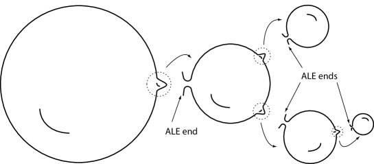
Figure 2. A bubble tree with several levels of scaling. The dotted circles enclose the regions of singularity formation, and are close to orbifold singularities (in the Cheeger-Gromov sense). The curved arrows represent these regions viewed through a powerful microscope.

7.1. Bubble-tree structure for hyperbolic monopole metrics

The following theorem describes the bubble formation for compactified LeBrun metrics.

Theorem 7.1.

Let $(M,g_{i})$ be a sequence of $n$-pointed LeBrun metrics with monopole points $\{p_{i,1},\dots,p_{i,n}\}$. Assume that as $i\rightarrow\infty$ that these points converge to

(7.1) $$\{p_{i,1},\dots,p_{i,n}\}\rightarrow\{m_{1}\cdot p_{\infty,1},\dots,m_{k}\cdot p_{\infty,k}\},$$

as $i\rightarrow\infty$ with $p_{\infty,j}\in\mathcal{H}^{3}$ for $1\leq j\leq k_{1}$ and $p_{\infty,j}\in\partial\mathcal{H}^{3}$ for $k_{1}<j\leq k$, allowing for multiplicity. Then there exist metrics $\hat{g}_{j}$ on the conformal compactification so that $(\hat{M},\hat{g}_{j})$ converges to the compactified LeBrun orbifold

(7.2) $$(\hat{M},\hat{g}_{j})\rightarrow\big{(}M_{\infty},\hat{g}_{{\rm{LB}}}(m_{1}\cdot p_{\infty,1},\dots,m_{k_{1}}\cdot p_{\infty,k_{1}})\big{)},$$

as $j\rightarrow\infty$ in the Cheeger-Gromov sense. There are finitely many bubbles, and the bubble-tree structure is as follows. For each subcollection of points limiting to a finite point with multiplicity greater than one, the bubble-tree structure is a tree of Gibbons-Hawking multi-Eguchi-Hanson orbifold ALE spaces. For each subcollection of points limiting to a boundary point, then a LeBrun orbifold AF metric is the first bubble at that point, with subsequent bubbles being Gibbons-Hawking orbifolds as in the previous case. The neck regions are modeled on annuli in Euclidean spaces $\mathbb{R}^{4}/\mathbb{Z}_{k}$, with the group action as in (2.2).

Proof.

By a sequence of conformal transformations, we normalize the sequence so that $p_{i,1}=(0,0,1)$. Choose a conformal factor $u:\mathcal{H}^{3}\rightarrow\mathbb{R}_{+}$ so that $\hat{g}_{i}=u^{2}g_{i}$ is a sequence of smooth metrics on the compactification $\hat{M}$ as follows. Viewing $\mathcal{H}^{3}$ as the upper half space, without loss of generality we may assume that the limiting boundary points lie in some compact set of the $(x,y,0)$-plane. We choose the compactifying conformal factor $u$ to be identically $1$ on some open neighborhood $U$ containing this compact set and such that $U$ also contains all monopole points. Furthermore, choose $u$ to be asymptotic to (5.1) on $\partial\mathcal{H}^{3}\setminus U$, so that $\hat{g}_{i}$ is a smooth metric on the compactification. To understand the bubble structure, we can therefore ignore the compactifying conformal factor in the following argument.

We first consider the case of several points limiting to a higher multiplicity point, say $m_{1}\cdot p_{\infty,1}$ with $m_{1}>1$. If all points limit to $p_{\infty,1}$ at a uniform rate, then we rescale the metric so that the points are minimally seperated by distance $1$. As in [LeB91, page 237], this is equivalent to rescaling the hyperbolic metric to become the flat metric, and the function $V$ limiting to the sum of Euclidean Green’s functions (without a constant). Thus the rescaled limit is a Gibbons-Hawking metric. If the points do not limit to $m_{1}\cdot p_{\infty,1}$ at a uniform rate, then we do the following. Rescale the metric the smallest amount so that the maximum distance between these points is $1$. We will then see several “clusters” of points limiting to distinct points in a unit ball. Thus the limit will be a Gibbons-Hawking ALE orbifold. At each orbifold point $q$ of this limit, we return to the original sequence and rescale so that the maximum distance between the subcollection of points limiting to $q$ in the first rescaling is $1$. At this scaling, we will then see several new subclusters limiting to distinct points in a unit ball, so again we find Gibbons-Hawking orbifolds at a different scale.

Next, for a subcollection of points limiting to a boundary point, by a conformal transformation, we arrange so that this cluster of points is contained in a unit ball around some finite point in $\mathcal{H}^{3}$, say $p=(0,0,1)$. The pointed limit (based at $p$) of such rescaled metrics is a LeBrun hyperbolic monopole AF orbifold metric (since in this gauge, all other points will limit to $\partial\mathcal{H}^{3}$. This is conformal related to the original, but it is easy to see that in the original scaling, precisely this AF orbifold metric bubbles off. We will illustrate this in a simple case, the general argument is the same. Consider the case of 2 monopole points. Let $p_{j,1}=(0,0,1),p_{j,2}=(0,0,j^{-1})$. Let $\phi_{j}(x,y,z)=(jx,jy,jz)$, this is a hyperbolic isometry. By [HV09, Section 2], there is a lift ${\Phi}_{j}$ of $\phi$ preserving the connection form. We then have

(7.3) $${\Phi}_{j}^{*}(g_{LB}(p_{j,1},p_{j,2}))=j^{2}\Big{(}g_{LB}\big{(}(0,0,j),(0,0,1)\big{)}\Big{)}.$$

In other words, we see that a scaling of the original metric is isometric to another LeBrun metric. Consequently, the bubble will be a LeBrun AF metric (in this case a Burns metric). In general, there could be clusters of points tending towards $\partial\mathcal{H}^{3}$, and then clearly all deeper bubbles at such points will be Gibbons-Hawking orbifold metrics, as in the first paragraph.

Since the number of monopole points is bounded by $n$, this procedure must terminate in finitely many steps, and thus there are finitely many non-trivial bubbles. A trivial bubble, or neck region, will arise at any intermediate scaling between a non-trivial ALE space, and the previous orbifold point onto which is it glued. All of the above ALE spaces are Kähler and have an ALE-coordinate system in which the group action is as in (2.2), so the structure of the neck regions is clearly as stated. ∎

Remark 7.2.

To clarify, we explain the above procedure in two cases. Consider the case of $3$ points, and normalize so that $p_{j,1}=(0,0,1)$. Choose $p_{j,2}$ and $p_{j,3}$ to be at distance $j^{-2}$ from each other, but such that both of these are at distance $j^{-1}$ from $p_{j,1}$. In this case, the original limit is a LeBrun metric with a single multiplicity $3$ point. To see the first bubble, we rescale the picture so that the distance between $p_{j,1}$ and $p_{j,2}$ is $1$. Thus the first bubble will be a Gibbons-Hawking orbifold with one point of multiplicity $1$, and another point of multiplicity $2$. The second, deepest, bubble will rescale so that $p_{j,2}$ and $p_{j,3}$ are at distance $1$, and this bubble will be a Gibbons-Hawking metric with $2$ points of multiplicity $1$, which is none other than the classical Eguchi-Hanson metric.

For the next example, consider again the case of $3$ points. Assume that $p_{j,1}=(0,0,1)$, and choose $p_{j,2}$ and $p_{j,3}$ to limit to the boundary point $(0,0,0)$. The limit of the original sequence will be a LeBrun metric with a single monopole point (which we know is conformal to the Fubini-Study metric). To understand the bubbling, apply a conformal transformation so that $p_{j,2}$ and $p_{j,3}$ limit to $(0,0,1)$ (and then $p_{j,1}$ will limit to the boundary of hyperbolic space). The limit will now be a LeBrun AF metric with a single point of multiplicity $2$. This AF space will be the first bubble. Upon further rescaling to separate these two points, we find the second deepest bubble to be an Eguchi-Hanson metric.

7.2. Sobolev constants and Yamabe invariants

We proceed with the definition of the Sobolev constant.

Definition 7.3.

For $\hat{M}$ compact, we define the Sobolev constant $C_{S}$ as the best constant $C_{S}$ so that for all $f\in C^{0,1}(\hat{M})$ we have

(7.4) $$\|f\|_{L^{4}}\leq C_{S}\left(\|\nabla f\|_{L^{2}}+\|f\|_{L^{2}}\right).$$

For $M$ non-compact, $C_{S}$ is defined to be the best constant so that

(7.5) $$\|f\|_{L^{4}}\leq C_{S}\|\nabla f\|_{L^{2}},$$

for all $f\in C^{0,1}(M)$ with compact support.

We next prove the lower estimate on the Yamabe invariant in Theorem 1.2.

Theorem 7.4.

Let $(\hat{M},\hat{g})$ be a LeBrun self-dual conformal class on $n\#\mathbb{CP}^{2}$ with $n$ monopole points $\{p_{1},\dots,p_{n}\}$. Assume that all monopole point are contained in a compact set $\mathcal{K}\subset\mathcal{H}^{3}$. Then there exists a constant $\delta_{n}>0$ depending only upon $n,\mathcal{K}$ such that

(7.6) $$0<\delta_{n}\leq Y(\hat{M},[\hat{g}]).$$

Proof.

Let $\hat{g}_{{\rm{LB}},i}$ be a sequence of such LeBrun metrics, with monopole points $p_{i,j}$, $j=1\dots n$, and assume that

(7.7) $$\{p_{i,1},\dots,p_{i,n}\}\rightarrow\{m_{1}\cdot p_{\infty,1},\dots,m_{k}\cdot p_{\infty,k}\},$$

as $i\rightarrow\infty$ with $p_{\infty,j}\in\mathcal{H}^{3}$ for $1\leq j\leq k$ allowing for multiplicity (from our assumption, there are no limit points on $\partial\mathcal{H}^{3}$). Inspired by [LNN97], let

(7.8) $$f_{i}=-(\rho_{i,1}+\dots+\rho_{i,n})/n,$$

where $\rho_{i,j}(\cdot)=d_{\mathcal{H}^{3}}(p_{i,j},\cdot)$. Without loss of generality, by conformal invariance, we may assume that $p_{i,1}=(0,0,1)$. Consider the conformally compactified $\tilde{g}_{i}=e^{2f_{i}}z^{-2}g_{{\rm{LB}},i}$, as in (3.11). Note that since all points are contained in a compact set around $p_{i,1}=(0,0,1)$, $f_{i}$ is bounded from below on any compact set, and $f_{i}(x)\sim-p_{i,1}(x)$ as $x\rightarrow\partial\mathcal{H}^{3}$. This implies that $\lambda<Vol(\tilde{g}_{i})<\Lambda$, for some positive constants $\lambda$ and $\Lambda$. The same argument in Theorem 7.1, then shows that $\tilde{g}_{i}$ converges to a non-trivial limiting orbifold $(\hat{M}_{\infty},\hat{g}_{\infty})$ with finitely many ALE orbifold bubbles (our conformal factor now varies with $i$, but it remains bounded and strictly positive near the singularities, so the same argument applies). Since $|\nabla\rho_{i,j}|=1$, this implies the inequality

(7.9) $$|\nabla f_{i}|^{2}<1/n.$$

From (3.12), we estimate the scalar curvature

$$R_{\tilde{g}_{i}} =6e^{-2f_{i}}V_{i}^{-1}(-1-\Delta f_{i}-|\nabla f_{i}|^{2})$$

$$>6e^{-2f_{i}}V_{i}^{-1}(-2-\Delta f_{i})=6e^{-2f_{i}}V_{i}^{-1}n^{-1}\sum_{j}(-2+\Delta\rho_{i,j}),$$

where $V_{i}$ is defined in (2.7), corresponding to the $n$ monopole points $p_{i,j}$. Using Lemma 3.1, we obtain the estimate

(7.10) $$R_{\tilde{g}_{i}}>24e^{-2f_{i}}V_{i}^{-1}n^{-1}\sum_{j}e^{-2\rho_{i,j}}V_{i,j},$$

where $V_{i,j}=1+\Gamma_{p_{i,j}}$. For each $j$, the function $V_{i}^{-1}V_{i,j}$ is smooth and uniformly positive (with a lower bound independent of $i$), so we have

(7.11) $$R_{\tilde{g}_{i}}>Ce^{-2f_{i}}\sum_{j}e^{-2\rho_{i,j}},$$

for some constant $C>0$. Obviously, for some $j_{0}$ we must have

(7.12) $$\frac{1}{n}\sum_{j}\rho_{i,j}\geq\rho_{i,j_{0}}.$$

Therefore, we have the estimate

(7.13) $$R_{\tilde{g}_{i}}>\delta>0.$$

We also claim that there is a uniform bound on the Sobolev constant (7.4). The limit space $(\hat{M}_{\infty},\hat{g}_{\infty})$ has bounded Sobolev constant (7.4) since it is a compact orbifold. Furthermore, all of the bubbles are ALE orbifolds, which have bounded Sobolev constants (7.5) by [Bar86], and each are glued onto the previous orbifold by Euclidean neck regions. Therefore, using a standard partition of unity argument (at possibly several scales) and scale invariance of the Sobolev constant (7.5), it follows that the Sobolev constant of the sequence is uniformly bounded. This is proved in detail in [Joy03, Proposition 2.2], and the generalization to this case is straightforward, so we omit the details.

To finish the proof, we include the following standard argument. Assume by contradiction that there is a sequence of unit-volume Yamabe minimizers in each conformal class $g_{Y,i}=v_{i}^{2}\tilde{g}_{i}$ with $R_{i}\rightarrow 0$ as $i\rightarrow\infty$, where $R_{i}$ is the (constant) scalar curvature of $g_{Y,i}$. The Yamabe equation is

(7.14) $$-6\Delta v_{i}+R(\tilde{g}_{i})v_{i}=R_{i}v_{i}^{3}.$$

Multiply by $v_{i}$ and integrate to get

(7.15) $$6\int|\nabla v_{i}|^{2}dV_{\tilde{g}_{i}}+\int R(\tilde{g}_{i})v_{i}^{2}dV_{\tilde{g}_{i}}=\int R_{i}v_{i}^{4}dV_{\tilde{g}_{i}}=R_{i}Vol(g_{Y,i})=R_{i}.$$

The right hand side limits to zero, therefore the left-hand side does also as $i\rightarrow\infty$. From (7.13), $R(\tilde{g}_{i})$ is uniformly positive, so the $W^{1,2}$ norm of $v_{i}$ can be made arbitrarily small. Using the uniform Sobolev inequality and lower volume bound for $\tilde{g}_{i}$,

(7.16) $$1=Vol(g_{Y,i})^{1/4}=\|v_{i}\|_{L^{4}}\leq C_{S}(\tilde{g}_{i})\left(\|\nabla v_{i}\|_{L^{2}}+\|v_{i}\|_{L^{2}}\right)\leq C^{\prime}\|v_{i}\|_{W^{1,2}},$$

which is a contradiction for $i$ sufficiently large. ∎

7.3. Convergence of constant scalar curvature metrics

We are now in a position to describe the possible limits of the Yamabe minimizers. The following Theorem implies the main part of Theorem 1.2.

Theorem 7.5.

Fix $n$, and let $(M,g_{i})$ be an arbitrary sequence of $n$-pointed LeBrun metrics, with conformal compactifications $(\hat{M},[\hat{g}_{i}])$. Assume that there exists a constant $\delta_{n}$ such that

(7.17) $$0<\delta_{n}\leq Y(\hat{M},[\hat{g}_{i}]).$$

Let $g_{Y,i}\in[\hat{g}_{i}]$ be a sequence of unit volume Yamabe minimizers. Then there exists a subsequence $g_{Y,j},\{j\}\subset\{i\},$ which converges to either $(1)$ a constant scalar curvature metric on a $k$-pointed LeBrun orbifold, $1\leq k\leq n$, or $(2)$ a single football metric, that is, $S^{4}/\mathbb{Z}_{m}$ with the round metric, for $2\leq m\leq n$.

Proof.

As in Theorem 7.1, we choose a compactification with fixed conformal factor $\tilde{g}_{i}\in[g_{i}]$, so that the sequence $(\hat{M},\tilde{g}_{i})$ will limit to a compactified LeBrun orbifold, with each bubble-tree consisting of a string of multi-Eguchi-Hanson orbifolds, and possibly other AF LeBrun orbifold metrics (in case some monopole points limit to the boundary of $\mathcal{H}^{3}$). Call this limit space $(\hat{M}_{\infty},\hat{g}_{\infty})$, and the finite singular set of convergence $S\subset\hat{M}_{\infty}$. We write the sequence of unit volume Yamabe minimizers in each conformal class as $g_{Y,i}=v_{i}^{2}\tilde{g}_{i}$. Let $R_{i}$ denote the scalar curvature of $g_{Y,i}$. By passing to a subsequence, assume that $\lim_{i\rightarrow\infty}R_{i}=R_{\infty}$. From the assumption (7.17), $R_{\infty}>\delta>0$.

The assumption (7.17) implies that the Yamabe minimizers $g_{Y,i}$ satisfy a uniform Sobolev inequality of the following form [TV05b, Proposition 3.1]

(7.18) $$\|f\|_{L^{4}}\leq C_{S}\|\nabla f\|_{L^{2}}+Vol^{-1/4}\|f\|_{L^{2}},$$

for any $f\in C^{0,1}(\hat{M})$. The $L^{2}$-norm of the curvature is uniformly bounded, as seen above in Section 6. We may therefore quote the compactness theorem of [TV05b, Theorem 1.1] to obtain a subsequence converging to a multi-fold limit. The Sobolev inequality (7.18) and $b_{1}(\hat{M})=0$ together imply that the limit must be an irreducible orbifold [TV05b, Proposition 7.2].

Let $C_{i}=\max_{\hat{M}}u_{i}$. If $C_{i}$ remains bounded from above, then we argue as follows. On any compact subset $D\subset\hat{M}_{\infty}\setminus S$, we have a Harnack inequality (since the conformal factors are bounded from above, and the sequence is smoothly converging away from the singular set). This implies that the conformal factors $u_{i}$ will either have a strictly positive limit on $\hat{M}_{\infty}$ or will uniformly crash to zero on $\hat{M}_{\infty}$. The latter case cannot happen since $Vol(g_{Y,i})=1$. Consequently, the limit must be a CSC (constant scalar curvature) metric conformal to $(\hat{M}_{\infty},\hat{g}_{\infty})$, and we are in Case (1).

So we next assume that $C_{i}\rightarrow\infty$ as $i\rightarrow\infty$. Let $x_{i}$ be points such that $u_{i}(x_{i})=C_{i}$. We first assume that $x_{i}\rightarrow x\in\hat{M}_{\infty}\setminus S$. Then the usual conformal dilation argument says that a bubble is forming on the smooth part [Sch91]. To summarize, this is by looking at the rescaled functions $\tilde{u}_{i}(y)=C_{i}^{-1}u_{i}(C_{i}^{-1}y)$. By elliptic theory, this sequence has a subseqence converging to a positive solution of $-6\Delta u=R_{\infty}u^{3}$ on $\mathbb{R}^{4}$, satisfying $u(0)=1$. From our assumption on the Yamabe invariant, $R_{\infty}>\delta>0$. By Caffarelli-Gidas-Spruck [CGS89], the limit must be the spherical metric. This implies that the Yamabe invariant satisfies $Y(\hat{M},[\tilde{g}_{i}])\gtrsim Y(S^{4},[g_{S}])$, for $i$ large, which contradicts Theorem 3.2 above. Therefore, we must have $x_{i}\rightarrow p\in S$ as $i\rightarrow\infty$. Let $(X_{1},g_{1})$ be the first bubble at $p$. Assume that, after the rescaling the sequence to limit to $(X_{1},g_{1})$ (pointed convergence based at $p$), $x_{i}$ limits to a finite point of $X_{1}$. The same conformal dilation argument shows that the rescaled conformal factor (with $g_{1}$ as background metric) must be bounded from above. Away from the singular points of convergence $p_{1,j^{\prime}},j^{\prime}=1\dots k_{1}$, we again have a Harnack inequality. So the rescaled conformal factor either (a) limits identically to zero away from the singlar points, or (b) has a finite positive limit everywhere. In Case (b), the limit of the original sequence must then be a CSC metric on the conformal compactification $(\hat{X}_{1},\hat{g}_{1})$, since this is the only possible irreducible orbifold limit. If $X_{1}$ is an Eguchi-Hanson orbifold, this cannot happen by Proposition 4.2. So the only possibility in Case (b) is that $(X_{1},g_{1})$ is an orbifold LeBrun AF metric, whose compactification is Case (1). Case (a) splits into two possibilities. Case (a1) is that $x_{i}$ will limit to $\infty$ in $(X_{1},g_{1})$. In this case, the only possible irreducible orbifold limit will be a metric on the compactification of the “neck” region. This follows since all ALE spaces in the bubble tree described in Theorem 7.1 have one end, the only possible neck regions are modeled on $\mathbb{R}^{4}/\mathbb{Z}_{m}$. The only CSC metric on the compactification of this is the $S^{4}/\mathbb{Z}_{m}$-football metric, by the Obata-Tashiro Theorem [Oba72, Tas65]. Therefore, Case (a1) is exactly Case (2). Case (a2) is that $x_{i}$ limits to one of the singular points of convergence of $X_{1}$ in this scaling. We then repeat the above argument around this singular point. In general, we repeat the entire argument at different scalings to see that the limit must be (i) a CSC metric on exactly one of the compactified orbifolds in the bubble-tree, or (ii) limit occurring on a neck region. For Case (i), the Gibbons-Hawing orbifolds do not admit CSC metrics by Proposition 4.2, so Case (i) is exactly Case (1). The argument above shows that Case (ii) is exactly Case (2).

Finally, in Case (1), the limit can never be a compactified $0$-pointed LeBrun metric. This is conformal to $S^{4}$ with the round metric, and the only CSC metrics in this conformal class are of constant curvature [Oba72], so have maximal Yamabe invariant. This would contradict (1.4). This also proves $2\leq m$ in Case (2). ∎

7.4. Completion of proofs of Theorems 1.1 and 1.5

The Yamabe invariant for $n=2,3$ is stricly positive by Proposition 6.1. For Theorem 1.1, as $d_{H}(p_{1},p_{2})\rightarrow\infty$, Theorem 7.5 says the only possible limit is the compactified $1$-pointed LeBrun metric, since Case (2) obviously does not happen. This is conformal to the Fubini-Study metric, which is the unique CSC metric in its conformal class by Obata’s Theorem [Oba72]. We note that the behavior of the Yamabe-minimizer on a connect sum is typically non-symmetric [Kob87, Joy03]. Since the Yamabe minimizers must limit to the Fubini-Study metric, it is then obvious that for $d_{H}(p_{1},p_{2})$ very large, the Yamabe minimizers cannot be invariant under the conformal involution which flips the two monopole points (see Section 5.1). Therefore, there must always be at least two distinct Yamabe minimizers, which are related by this conformal involution.

We next address the $K$-symmetric limit to $S^{4}$. The existence of $K$-symmetric minimizers follows from [Heb96]. Again, by [TV05b] we can find a subsequence converging to a multi-fold, but which now may have reducible points. But from the estimate on the $K$-Yamabe invariant in Theorem 5.4, as $d_{H}(p_{1},p_{2})\rightarrow\infty$, it is clear that the only possibility for a $K$-Yamabe minimizer is $S^{4}$ with the round metric. This follows because a reflection interchanging the two monopole point is clearly not an isometry of the two Yamabe minimizers, so these are not possible limits. From the arguments in the proof of Theorem 7.5, another possible limit is $\mathbb{CP}^{2}\vee\mathbb{CP}^{2}$, with the Fubini-Study metric scaled to have $Vol=1/2$ on each factor. But this cannot occur since the Yamabe invariant of this limit is $24\pi>8\pi\sqrt{6}=Y(S^{4},g_{S})$, and this would contradict Theorem 5.4. Similarly, the limit $\mathbb{CP}^{2}\vee S^{4}$ cannot happen either. Therefore, any sequence of Yamabe minimizers must concentrate entirely in the neck region. The only possible limit is then $S^{4}$ with the round metric, with Burns metrics bubbling off at the 2 singular points of convergence. This follows since any reducible limit would be several $S^{4}$-s wedged together, which would have Yamabe invariant strictly larger than $8\pi\sqrt{6}$.

Remark 7.6.

As shown in [HV09], $G$ is generated by $K$ and an extra involution $\Lambda$ which is not a lift of a hyperbolic isometry, and is quite difficult to describe explicitly. It is likely that as $d(p_{1},p_{2})\rightarrow\infty$, the $G$-symmetric metric must also limit to $S^{4}$. But since the test metric in (5.12) is not invariant under $\Lambda$, we cannot say this for certain.

The fourth metric in Theorem 1.1 is obtained by adapting the CSC-gluing argument of Joyce to this problem [Joy03], see also [MPU95]. Recall that the Euclidean Schwarzschild metric in dimension $n$ is defined as

(7.19) $$g=\left(1+\frac{m}{(n-1)r^{n-2}}\right)^{\frac{4}{n-2}}g_{0},$$

on $\mathbb{R}^{n}\setminus\{0\}$, where $g_{0}$ is the Euclidean metric, and $m>0$ is the mass parameter. This metric is scalar-flat, locally conformally flat, and AF with two ends. One chooses a conformal factor which is close to the Fubini-Study metric on neighborhoods of the monopole points, and is close to a scaled-down Schwarzschild neck region in between; this will be the approximate CSC-metric. One then uses the implicit function theorem, together with the crucial fact that the Fubini-Study metric is CSC-nondegenerate, to perturb to a CSC metric. This adaptation is straightforward, but since the argument is quite lengthy, we omit the details due to space considerations.

As $d_{H}(p_{1},p_{2})\rightarrow 0$, Case (1) in Theorem 7.5 could only be a compactified LeBrun metric with a single point of multiplicity $2$. This is conformal (minus the orbifold point) to the Eguchi-Hanson metric, which does not admit any CSC metric by Theorem 1.3, so this case cannot happen. Consequently, the only possibility for the limit is the $S^{4}/\mathbb{Z}_{2}$-football with the round metric (since the limit of Yamabe minimizers must be irreducible). Similarly, Theorem 1.3 implies that as $d_{H}(p_{1},p_{2})\rightarrow 0$, the only possible $K$-symmetric limit is the $S^{4}/\mathbb{Z}_{2}$-football with the round metric. To see this, again the only concentration can occur in the neck region, which is $\mathbb{R}^{4}/\mathbb{Z}_{2}$. The limit no longer has to be irreducible. But the lowest energy reducible limit would be the wedge of two $S^{4}/\mathbb{Z}_{2}$-footballs, whose Yamabe energy is $8\pi\sqrt{6}$. However, since in this case the points are not limiting to the boundary of $\mathcal{H}^{3}$, Theorem 5.4 shows that the Yamabe energy must be strictly less than $8\pi\sqrt{6}$, so this cannot happen, and therefore the limit must be the irreducible $S^{4}/\mathbb{Z}_{2}$-football.

For the first case in Theorem 1.5, as $p_{3}\rightarrow p_{2}$, the only possible limits from Theorem 7.5 are Case (1): a compactified LeBrun metric with a single monopole point, and another multiplicity $2$ point, or Case (2): a $S^{4}/\mathbb{Z}_{2}$-football with the round metric. However, under the assumptions of Theorem 1.5, (4.11) says the Yamabe invariant is strictly less than that of the $S^{4}/\mathbb{Z}_{2}$-football, so the limit must be Case (1).

Finally, for the last case in Theorem 1.5, as $p_{3}\rightarrow\partial\mathcal{H}^{3}$, the Yamabe invariant is strictly less than that of $g_{FS}$ by Theorem 3.2. Thus the only possible limit is Case (1), a $2$-pointed LeBrun compactified metric.

8. Questions

We conclude with a list of questions.

• What is the optimal lower bound for the Yamabe invariant in (1.5) for $n\geq 2$? We conjecture that $\delta_{n}=Y_{orb}(S^{4}/\mathbb{Z}_{n},[g_{S}])$; this is true for $n=2$, as seen above in Theorem 1.1. Furthermore, the assumption that the points are contained in a compact set $\mathcal{K}\subset\mathcal{H}^{3}$ should not be necessary. Removing this assumption would imply that the moduli space of Yamabe minimizing LeBrun metrics has a nice compactification for any $n$. As seen above, this is true for $n=2,3$.

• Does the compactified LeBrun metric on $\mathcal{O}(-n)$ admit a CSC metric for $n\geq 3$? The answer is no for $n=2$ since this is the compactified Eguchi-Hanson metric, which was ruled out by Theorem 1.3. For $n\geq 3$, Theorem 1.4 rules out any symmetric solution, but is there a non-symmetric solution? Furthermore, as shown in Theorem 7.1, if all monopole points approach a single point at a uniform rate, the bubble-tree structure is a compactified LeBrun negative-mass metric on $\mathcal{O}(-n)$, with a Gibbons-Hawking multi-Eguchi-Hanson bubbling off. From the arguments in Section 7, the limit of the Yamabe minimizers could limit to either a CSC metric on compactified $\mathcal{O}(-n)$, or to the $S^{4}/\mathbb{Z}_{n}$-football (since the compactified GH metric does not admit a CSC metric by Theorem 1.3). Which one actually happens for $n\geq 3$?

• Except for the case of a single monopole point with multiplicity $n$, does a $[\hat{g}_{LB}]$ orbifold conformal class always admit a CSC metric?

• In Theorem 1.1, for $n=2$ we determined the limiting behavior of the $K$-Yamabe minimizers as $d(p_{1},p_{2})\rightarrow\infty$ (the limit is $S^{4}$). Recall that $K$ is an index $2$ subgroup of full conformal group $G$. What is the limit of the $G$-Yamabe minimizers?

• Are CSC metrics on compactified LeBrun metrics CSC nondegenerate? If so, then it would then be possible to apply the Joyce gluing technique to obtain more non-Yamabe-minimizing examples.

• LeBrun metrics with torus action are a special case of Joyce metrics [Joy95]. These depend on a choice of points on the boundary of hyperbolic $2$-space. What happens as these metrics degenerate?

References

- [AB03] K. Akutagawa and B. Botvinnik, Yamabe metrics on cylindrical manifolds, Geom. Funct. Anal. 13 (2003), no. 2, 259–333.
- [AB04] Kazuo Akutagawa and Boris Botvinnik, The Yamabe invariants of orbifolds and cylindrical manifolds, and -harmonic spinors, J. Reine Angew. Math. 574 (2004), 121–146.
- [AKL89] Michael T. Anderson, Peter B. Kronheimer, and Claude LeBrun, Complete Ricci-flat Kähler manifolds of infinite topological type, Comm. Math. Phys. 125 (1989), no. 4, 637–642.
- [Aku94] Kazuo Akutagawa, Yamabe metrics of positive scalar curvature and conformally flat manifolds, Differential Geom. Appl. 4 (1994), no. 3, 239–258.
- [Aku96] by same author, Convergence for Yamabe metrics of positive scalar curvature with integral bounds on curvature, Pacific J. Math. 175 (1996), no. 2, 307–335.
- [Aku10] by same author, Computations of the orbifold Yamabe invariant, arXiv.org:1009.3576, 2010.
- [And89] Michael T. Anderson, Ricci curvature bounds and Einstein metrics on compact manifolds, J. Amer. Math. Soc. 2 (1989), no. 3, 455–490.
- [And05] by same author, Orbifold compactness for spaces of Riemannian metrics and applications, Math. Ann. 331 (2005), no. 4, 739–778.
- [Aub82] Thierry Aubin, Nonlinear analysis on manifolds. Monge-Ampère equations, Springer-Verlag, New York, 1982.
- [Ban90] Shigetoshi Bando, Bubbling out of Einstein manifolds, Tohoku Math. J. (2) 42 (1990), no. 2, 205–216.
- [Bar86] Robert Bartnik, The mass of an asymptotically flat manifold, Comm. Pure Appl. Math. 39 (1986), no. 5, 661–693.
- [CGS89] Luis A. Caffarelli, Basilis Gidas, and Joel Spruck, Asymptotic symmetry and local behavior of semilinear elliptic equations with critical Sobolev growth, Comm. Pure Appl. Math. 42 (1989), no. 3, 271–297.
- [CGY02] Sun-Yung A. Chang, Matthew J. Gursky, and Paul C. Yang, An equation of Monge-Ampère type in conformal geometry, and four-manifolds of positive Ricci curvature, Ann. of Math. (2) 155 (2002), no. 3, 709–787.
- [CLW08] Xiuxiong Chen, Claude Lebrun, and Brian Weber, On conformally Kähler, Einstein manifolds, J. Amer. Math. Soc. 21 (2008), no. 4, 1137–1168.
- [CQY07] Sun-Yung A. Chang, Jie Qing, and Paul Yang, On a conformal gap and finiteness theorem for a class of four-manifolds, Geom. Funct. Anal. 17 (2007), no. 2, 404–434.
- [CW07] Xiuxiong Chen and Brian Weber, Moduli spaces of critical riemannian metrics with norm curvature bounds, arXiv.org:0705.4440, 2007.
- [DF89] S. Donaldson and R. Friedman, Connected sums of self-dual manifolds and deformations of singular spaces, Nonlinearity 2 (1989), no. 2, 197–239.
- [Flo91] Andreas Floer, Self-dual conformal structures on , J. Differential Geom. 33 (1991), no. 2, 551–573.
- [GH78] G. W. Gibbons and S. W. Hawking, Gravitational multi-instantons, Physics Letters B 78 (1978), no. 4, 430–432.
- [GV03] Matthew J. Gursky and Jeff A. Viaclovsky, A fully nonlinear equation on four-manifolds with positive scalar curvature, J. Differential Geom. 63 (2003), no. 1, 131–154.
- [Heb96] Emmanuel Hebey, From the Yamabe problem to the equivariant Yamabe problem, Actes de la Table Ronde de Géométrie Différentielle (Luminy, 1992), Sémin. Congr., vol. 1, Soc. Math. France, Paris, 1996, Joint work with M. Vaugon, pp. 377–402.
- [Hit79] N. J. Hitchin, Polygons and gravitons, Math. Proc. Cambridge Philos. Soc. 85 (1979), no. 3, 465–476.
- [Hit97] by same author, Einstein metrics and the eta-invariant, Boll. Un. Mat. Ital. B (7) 11 (1997), no. 2, suppl., 95–105.
- [Hon10] Nobuhiro Honda, Degenerations of LeBrun twistor spaces, arXiv.org:1001.3461, 2010.
- [HV09] Nobuhiro Honda and Jeff Viaclovsky, Conformal symmetries of self-dual hyperbolic monopole metrics, arXiv.org:0902.2019, 2009.
- [Joy95] Dominic D. Joyce, Explicit construction of self-dual -manifolds, Duke Math. J. 77 (1995), no. 3, 519–552.
- [Joy03] Dominic Joyce, Constant scalar curvature metrics on connected sums, Int. J. Math. Math. Sci. (2003), no. 7, 405–450.
- [Kob87] Osamu Kobayashi, Scalar curvature of a metric with unit volume, Math. Ann. 279 (1987), no. 2, 253–265.
- [Kro89] P. B. Kronheimer, The construction of ALE spaces as hyper-Kähler quotients, J. Differential Geom. 29 (1989), no. 3, 665–683.
- [Küh88] Wolfgang Kühnel, Conformal transformations between Einstein spaces, Conformal geometry (Bonn, 1985/1986), Aspects Math., E12, Vieweg, Braunschweig, 1988, pp. 105–146.
- [LeB88] Claude LeBrun, Counter-examples to the generalized positive action conjecture, Comm. Math. Phys. 118 (1988), no. 4, 591–596.
- [LeB91] by same author, Explicit self-dual metrics on , J. Differential Geom. 34 (1991), no. 1, 223–253.
- [LNN97] Claude LeBrun, Shin Nayatani, and Takashi Nitta, Self-dual manifolds with positive Ricci curvature, Math. Z. 224 (1997), no. 1, 49–63.
- [LP87] John M. Lee and Thomas H. Parker, The Yamabe problem, Bull. Amer. Math. Soc. (N.S.) 17 (1987), no. 1, 37–91.
- [MPU95] Rafe Mazzeo, Daniel Pollack, and Karen Uhlenbeck, Connected sum constructions for constant scalar curvature metrics, Topol. Methods Nonlinear Anal. 6 (1995), no. 2, 207–233.
- [Nak90] Hiraku Nakajima, Self-duality of ALE Ricci-flat -manifolds and positive mass theorem, Recent topics in differential and analytic geometry, Academic Press, Boston, MA, 1990, pp. 385–396.
- [Nak94] by same author, A convergence theorem for Einstein metrics and the ALE spaces, Selected papers on number theory, algebraic geometry, and differential geometry, Amer. Math. Soc. Transl. Ser. 2, vol. 160, Amer. Math. Soc., Providence, RI, 1994, pp. 79–94.
- [Oba72] Morio Obata, The conjectures on conformal transformations of Riemannian manifolds, J. Differential Geometry 6 (1971/72), 247–258.
- [Po86] Y. Sun Poon, Compact self-dual manifolds with positive scalar curvature, J. Differential Geom. 24 (1986), no. 1, 97–132.
- [Rat06] John G. Ratcliffe, Foundations of hyperbolic manifolds, second ed., Graduate Texts in Mathematics, vol. 149, Springer, New York, 2006.
- [Sch84] Richard Schoen, Conformal deformation of a Riemannian metric to constant scalar curvature, J. Differential Geom. 20 (1984), no. 2, 479–495.
- [Sch91] Richard M. Schoen, On the number of constant scalar curvature metrics in a conformal class, Differential geometry, Longman Sci. Tech., Harlow, 1991, pp. 311–320.
- [Tas65] Yoshihiro Tashiro, Complete Riemannian manifolds and some vector fields, Trans. Amer. Math. Soc. 117 (1965), 251–275.
- [Tia90] G. Tian, On Calabi’s conjecture for complex surfaces with positive first Chern class, Invent. Math. 101 (1990), no. 1, 101–172.
- [TV05a] Gang Tian and Jeff Viaclovsky, Bach-flat asymptotically locally Euclidean metrics, Invent. Math. 160 (2005), no. 2, 357–415.
- [TV05b] by same author, Moduli spaces of critical Riemannian metrics in dimension four, Adv. Math. 196 (2005), no. 2, 346–372.
- [TV08] by same author, Volume growth, curvature decay, and critical metrics, Comment. Math. Helv. 83 (2008), no. 4, 889–911.