Quantum Monte Carlo study of the ground state of the two-dimensional Fermi fluid

Abstract

We have used the variational and diffusion quantum Monte Carlo methods to calculate the energy, pair correlation function, static structure factor, and momentum density of the ground state of the two-dimensional homogeneous electron gas. We have used highly accurate Slater-Jastrow-backflow trial wave functions and twist averaging to reduce finite-size effects where applicable. We compare our results with others in the literature and construct a local-density-approximation exchange-correlation functional for 2D systems.

I Introduction

The homogeneous electron gas (HEG) plays a key role in modern condensed-matter theory. It consists of a set of electrons moving in a uniform, inert, neutralizing background, and is the simplest fully-interacting quantum many-body model of condensed matter. The three-dimensional HEG models the behavior of the conduction electrons in metals and semiconductors, while the two-dimensional (2D) HEG models the behavior of electrons confined to surfaces and thin layers. Quantum Monte Carlo (QMC) methodsceperley_1980 ; foulkes_2001 have long played an important role in establishing the ground-state properties of the HEG. Most effort has gone into calculating the ground-state energy of different phases as a function of density, in order to establish the zero-temperature phase diagram.tanatar ; rapisarda ; ndd_2Dheg In this article, we report QMC calculations of some other properties of the 2D HEG of interest to condensed-matter physicists: the pair correlation function (PCF), static structure factor (SSF), and momentum density (MD). We also report energy data for high-density HEG’s. We have confined our attention to the fluid phase, which is the ground state at the densities typically encountered in experiments.

The PCF, especially the contact PCF $g(0)$, is a key ingredient in generalized-gradient-approximation exchange-correlation functionals for density functional theory (DFT) calculations. The PCF has been studied several times using QMC,tanatar ; rapisarda ; kwon_pcf ; gorigiorgi_pcf but the value of $g(0)$ at low densities has proved controversial because electrons approach one another infrequently, and the QMC results disagree with values calculated using ladder theory.qian Our QMC data, obtained using a different trial wave function from the earlier calculations, should help to clarify the situation. The SSF is related to the PCF by a Fourier transform. SSF data at small $k$ are needed to establish the long-range behavior of the PCF.

The MD of the HEG is of considerable importance in Fermi liquid theory. To our knowledge, the only QMC MD data to have been published for the 2D HEG are those of Tanatar and Ceperley,tanatar which used a relatively simple form of trial wave function. (A fit to QMC data generated by Conticonti is reported in Ref. giuliani, , but no details about the calculations are given.) Tanatar and Ceperley’s low-density MD shows a very strange feature: the MD is lower at zero momentum than it is at the top of the Fermi edge. It is clearly important to provide new QMC MD data, in order to establish whether this is a genuine property of the HEG.

Finally, we report ground-state energy data for paramagnetic Fermi fluids, which we use to parameterize a local-density-approximation exchange-correlation functional for use in DFT studies of 2D systems.

The rest of this article is arranged as follows. In Sec. II we describe the computational techniques used. In Sec. III we present the data we have generated. Finally, we draw our conclusions in Sec. IV. Densities are given in terms of the radius $r_{s}$ of the circle that contains one electron on average. We use Hartree atomic units ($\hbar=|e|=m_{e}=4\pi\epsilon_{0}=1$) throughout this article. All our QMC calculations were performed using the casino code.casino

II QMC calculations

II.1 Trial wave functions

In the variational quantum Monte Carlo (VMC) method, expectation values are calculated with respect to an approximate trial wave function, the integrals being performed by a Monte Carlo technique. In diffusion quantum Monte Carloceperley_1980 ; foulkes_2001 (DMC) the imaginary-time Schrödinger equation is used to evolve an ensemble of electronic configurations towards the ground state. The fermionic symmetry is maintained by the fixed-node approximation,anderson_1976 in which the nodal surface of the wave function is constrained to equal that of a trial wave function. The VMC algorithm generates electron configurations distributed according to the square of the trial wave function, while the DMC algorithm generates configurations distributed as the product of the trial wave function and its ground-state component.

Our trial wave functions consisted of Slater determinants of plane-wave orbitals multiplied by a Jastrow correlation factor. The Jastrow factor contained polynomial and plane-wave expansions in electron-electron separation.ndd_jastrow The orbitals in the Slater wave function were evaluated at quasiparticle coordinates related to the actual electron positions by backflow functions consisting of polynomial expansions in electron-electron separation.backflow The wave functions were optimized by variance minimizationumrigar_1988a ; ndd_newopt and linear-least-squares energy minimization.umrigar_emin

We simulated HEG’s in finite, square cells subject to periodic boundary conditions. The many-body Bloch theoremrajagopal states that the wave function $\Psi$ satisfies

$$\Psi({\bf r}_{1},\ldots,{\bf r}_{i}+{\bf R}_{s},\ldots,{\bf r}_{N})=\exp(i{\bf k}_{s}\cdot{\bf R}_{s})\Psi({\bf r}_{1},\ldots,{\bf r}_{N}),$$ (1)

where ${\bf R}_{s}$ is a simulation-cell lattice vector and ${\bf k}_{s}$ is the simulation-cell Bloch vector. In some of our calculations, and in previous QMC studies of the 2D HEG,tanatar ; rapisarda ; kwon it has been assumed that ${\bf k}_{s}={\bf 0}$. However, in our calculations of the energy, PCF, and SSF we performed twist averaging, in which expectation values are averaged over ${\bf k}_{s}$ in the first Brillouin zone of the simulation cell.lin_twist_av This procedure greatly reduces single-particle finite-size errors caused by shell-filling effects.

The high quality of our trial wave functions is demonstrated in Table 1, which shows QMC energies achieved using different levels of wave function for a 58-electron paramagnetic Fermi fluid of density parameter $r_{s}=5$ a.u. Backflow functions change the nodal surface of the trial wave function and can therefore improve the fixed-node DMC energy. In practice we find that backflow lowers the DMC energy substantially. Our VMC energies are significantly lower than those of Kwon et al.,kwon as is our Slater-Jastrow-backflow DMC energy. On the other hand, the Slater-Jastrow-backflow DMC energy of Attaccalite et al.attaccalite  is higher than that of Kwon et al. Our Slater-Jastrow DMC energy is slightly lower than that of Attaccalite et al., which in turn is lower than that of Kwon et al. Since the nodal surface is the same in the three calculations, these DMC energies really ought to agree. However, the trial wave function used by Kwon et al. is very much poorer than ours, as can be seen by comparing the VMC energies. Time-step and population-control biases in their DMC energies must be much greater, which may explain the discrepancy. The results of Attaccalite et al. have not been extrapolated to zero time step, hindering comparison. The VMC and DMC results of Rapisarda and Senatorerapisarda are in very close agreement with those of Kwon et al.kwon

Method	Energy (a.u. / elec.)		Var. (a.u.)		Frac. corr. en.
HF	$-0$.	$100\,222\,006$	$\cdots$		0	%
SJ-VMC	$-0$.	$148\,211\,0(8)$	$0$.	$019\,6$	96	.910(4)%
SJ-VMC∗	$-0$.	$146\,80(5)$	$\cdots$		94	.1(1)%
SJB-VMC	$-0$.	$149\,385\,1(6)$	$0$.	$007\,74$	99	.282(4)%
SJB-VMC∗	$-0$.	$148\,80(5)$	$\cdots$		98	.1(1)%
SJ-DMC	$-0$.	$149\,177(8)$	$\cdots$		98	.86(2)%
SJ-DMC∗	$-0$.	$149\,00(5)$	$\cdots$		98	.5(1)%
SJ-DMC†	$-0$.	$149\,134(9)$	$\cdots$		98	.77(2)%
SJB-DMC	$-0$.	$149\,741(2)$	$\cdots$		100	%
SJB-DMC∗	$-0$.	$149\,55(5)$	$\cdots$		99	.6(1)%
SJB-DMC†	$-0$.	$149\,518(9)$	$\cdots$		99	.55(2)%

Table 1: Energy, variance, and percentage of correlation energy retrieved using different methods for a 58-electron paramagnetic Fermi fluid of density parameter $r_{s}=5$ a.u. Twist averaging has not been used. “HF,” “SJ-VMC,” “SJB-VMC,” “SJ-DMC,” and “SJB-DMC” stand for Hartree-Fock theory, VMC with a Slater-Jastrow wave function, VMC with a Slater-Jastrow-backflow wave function, DMC with a Slater-Jastrow wave function, and DMC with a Slater-Jastrow-backflow wave function, respectively. The DMC energy data have been extrapolated to zero time step. The data marked with an asterisk were produced by Kwon et al.,kwon while the data marked with a dagger were generated by Attaccalite et al.attaccalite  at a time step of 0.1 a.u. (i.e. their data were not extrapolated to zero time step). The fraction of the correlation energy retrieved is computed on the assumption that our Slater-Jastrow-backflow DMC calculation retrieves 100% of the correlation energy.

We have optimized a three-electron term in the Jastrow factor (together with the two-electron Jastrow terms and backflow functions) for a paramagnetic 58-electron HEG at $r_{s}=5$ a.u. The three-electron term lowered the non-twist-averaged VMC energy from $-0.1493851(6)$ to $-0.1495111(5)$ a.u. per electron. The DMC energies at a time step of 0.1 a.u. without and with the three-body Jastrow factor are $-0.149742(2)$ and $-0.149740(2)$ a.u. per electron, respectively. As expected, the inclusion of the three-body term makes an insignificant difference to the DMC energy, because the DMC energy depends only on the nodal surface of the trial wave function, which is not directly affected by the Jastrow factor. We have therefore not used three-electron terms in our production calculations.

II.2 Evaluating expectation values

II.2.1 Evaluating the MD

Let $\Psi({\bf R})$ be the trial many-electron wave function, where ${\bf R}=({\bf r}_{1},\ldots,{\bf r}_{N})$. Suppose the first $N_{\uparrow}$ electrons are spin-up and the remainder are spin-down. The MD of spin-up electrons can be evaluated as

$$\rho({\bf k})=\left<\frac{1}{(2\pi)^{3}}\int\frac{\Psi({\bf r},{\bf r}_{2},\ldots,{\bf r}_{N})}{\Psi({\bf R})}\exp[i{\bf k}\cdot({\bf r}_{1}-{\bf r})]\,d{\bf r}\right>,$$ (2)

where the angled brackets denote an average over the set of electron configurations generated in the VMC and DMC algorithms (which are distributed as $|\Psi|^{2}$ and $|\Psi\Phi_{0}|$, respectively, where $\Phi_{0}$ is the ground-state component of $\Psi$). We have restricted our attention to paramagnetic and fully ferromagnetic HEG’s, so the total MD is equal to the spin-up MD. The integral in the expectation value of Eq. (2) is estimated by Monte Carlo sampling at each configuration ${\bf R}$ generated by the QMC algorithms, and the results are averaged. The use of a finite number of points in the evaluation of the integral at each ${\bf R}$ does not bias the QMC estimate of $\rho({\bf k})$.

Suppose our finite simulation cell has area $A$ and the simulation-cell Bloch vector is ${\bf k}_{s}$. We may write

$$\frac{\Psi({\bf r},{\bf r}_{2},\ldots,{\bf r}_{N})}{\Psi({\bf R})}=\frac{1}{A}\sum_{\bf G}c_{\bf G}({\bf R})\exp[i({\bf G}+{\bf k}_{s})\cdot{\bf r}],$$ (3)

where the $\{{\bf G}\}$ are the simulation-cell reciprocal lattice points. Hence it is clear that $\rho({\bf k})$ is only nonzero if ${\bf k}={\bf G}+{\bf k}_{s}$ for some ${\bf G}$. The MD is only defined for a discrete set of momenta at any given ${\bf k}_{s}$. One cannot twist average as such; instead, altering ${\bf k}_{s}$ leads to the MD being defined at a different set of momenta. We simply report MD’s obtained using ${\bf k}_{s}={\bf 0}$ (i.e., no twist was applied).

II.2.2 Evaluating the SSF

The SSF may be evaluated as

$$S({\bf k})=\frac{1}{N}\left[\left<\hat{n}({\bf k})\hat{n}(-{\bf k})\right>-\left<\hat{n}({\bf k})\right>\left<\hat{n}(-{\bf k})\right>\right],$$ (4)

where

$$\hat{n}({\bf k})=\sum_{i}\exp(-i{\bf k}\cdot{\bf r}_{i})$$ (5)

is the Fourier transform of the density operator. $S({\bf k})$ is only nonzero at simulation-cell ${\bf G}$ vectors, even if the simulation-cell Bloch vector is nonzero. We can twist average when we calculate $S({\bf G})$.

II.2.3 Evaluating the PCF

The spherically averaged PCF is

$$g(r)=\frac{\Omega}{4\pi r^{2}N^{2}}\left<\sum_{i\neq j}\delta(|{\bf r}_{i}-{\bf r}_{j}|-r)\right>,$$ (6)

which can be evaluated by binning the electron-electron distances in the configurations generated by the QMC algorithms. Twist averaging introduces no complications.

II.2.4 Extrapolated estimation

If $\hat{A}$ is an operator that does not commute with the Hamiltonian then the errors in the VMC and DMC estimates $A_{\rm VMC}$ and $A_{\rm DMC}$ of the expectation value of $\hat{A}$ are linear in the error in the trial wave function; however, the error in the extrapolated estimate $2A_{\rm DMC}-A_{\rm VMC}$ is quadratic in the error in the trial wave function.foulkes_2001 We have used extrapolated estimation in most of our calculations of expectation values. Examples of extrapolation are shown in Figs. 5 and 8, and the upper panel of Fig. 4. In each case the VMC, DMC, and extrapolated estimates are in good agreement, implying that the error resulting from the use of a DMC mixed estimate is small. Gori-Giorgi et al.gorigiorgi_pcf  used reptationreptation QMC to accumulate the PCF and SSF, in which pure expectation values are obtained with respect to the fixed-node ground-state wave function, so that extrapolation is unnecessary.

II.3 Time-step and population-control biases

Finite-time-step errors in the twist-averaged DMC energy were removed by linear extrapolation to zero time step. An example is shown in Fig. 1; it can be seen that the time-step bias is in fact very small in any case. We checked that the other expectation values were converged with respect to the time step: see Figs. 4 and 5. We used a target population of 1600 configurations in all our DMC calculations, making population-control bias negligible.

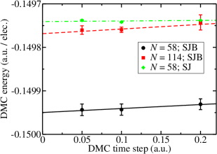
Figure 1: (Color online) Twist-averaged DMC energy against time step for paramagnetic Fermi fluids of density parameter $r_{s}=5$ a.u. at different system sizes $N$. “SJ” and “SJB” refer to Slater-Jastrow and Slater-Jastrow-backflow wave functions, respectively.

II.4 Finite-size bias

Expectation values obtained in a finite $N$-electron cell subject to periodic boundary conditions differ from the corresponding infinite-system values because of “single-particle” shell-filling effects, as well as the neglect of long-ranged correlations and the compression of the exchange-correlation hole into the simulation cell. Single-particle finite-size effects can be removed from the energy, the SSF, and the PCF by twist averaging, as explained in Sec. II.1. We have recently demonstrated that the finite-size error in the energy per particle in a 2D HEG falls off as $N^{-5/4}$, enabling us accurately to extrapolate QMC energies to infinite system size.ndd_fs For the PCF, SSF, and MD we simply verified that the QMC data had converged with respect to system size (see Figs. 5 and 8, and the lower panel of Fig. 4).

III Results

III.1 Energies

DMC energies of paramagnetic Fermi fluids at different densities and system sizes are shown in Table 2. Our results for the energies of different phases of the 2D HEG at low density are reported elsewhere.ndd_2Dheg At $r_{s}=5$ and 10 a.u., Rapisarda and Senatorerapisarda obtained infinite-system energies of $-0.1490(1)$ and $-0.08512(2)$ a.u. per particle using DMC with a Slater-Jastrow wave function. Kwon et al.kwon obtained DMC energies of $-0.2098(3)$, $-0.1495(1)$, and $-0.08536(2)$ a.u. per electron at $r_{s}=1$, 5, and 10, respectively, using a Slater-Jastrow-backflow wave function. Our DMC energies are somewhat lower than these data, as expected from the results shown in Table 1.

$r_{s}$ (a.u.)	$N$	DMC energy (a.u. / elec.)
1	50	$-0$.	$212\,5(2)$
1	74	$-0$.	$212\,2(2)$
1	114	$-0$.	$211\,6(3)$
1	$\infty$	$-0$.	$210\,4(6)$
5	58	$-0$.	$149\,95(2)$
5	114	$-0$.	$149\,77(1)$
5	$\infty$	$-0$.	$149\,63(3)$
10	58	$-0$.	$085\,504(5)$
10	74	$-0$.	$085\,52(1)$
10	114	$-0$.	$085\,445(3)$
10	$\infty$	$-0$.	$085\,399(6)$

Table 2: Twist-averaged DMC energy, extrapolated to zero time step, for $N$-electron paramagnetic Fermi fluids of density parameter $r_{s}$. Where $N=\infty$, the DMC energy has been extrapolated to infinite system size.

Let the correlation energy per electron $E_{c}$ be the difference between the ground-state energy per electron and the Hartree-Fock energy. We fit the form proposed by Attaccalite et al.attaccalite  to our correlation energies for paramagnetic HEG’s:

$$E_{c}=A_{0}+(B_{0}r_{s}+C_{0}r_{s}^{2}+D_{0}r_{s}^{3})\log\left(1+\frac{1}{E_{0}r_{s}+F_{0}r_{s}^{3/2}+G_{0}r_{s}^{2}+H_{0}r_{s}^{3}}\right),$$ (7)

where $A_{0}=-0.1925$, $B_{0}=\sqrt{2}(10-3\pi)/(3\pi)$, and $D_{0}=-A_{0}H_{0}$. We fit to the infinite-system DMC energies shown in Table 2 and also to the DMC energies of low-density paramagnetic HEG’s reported in Ref. ndd_2Dheg, (at $r_{s}=20$, 25, 30, 35, and 40 a.u.). Our fitting parameters are shown in Table 3 and the correlation energies of paramagnetic Fermi fluids obtained by different authors relative to that of Attaccalite et al. are shown in Fig. 2. Our correlation energies are lower than those of the other authors because of our use of flexible backflow functions. Equation (7) can be used as a local-density-approximation exchange-correlation functional in DFT calculations for 2D systems.

Parameter	Value
$A_{0}$	$-0$.	$192\,5$
$B_{0}$	$0$.	$086\,313\,631$
$C_{0}$	$0$.	$069\,795\,68$
$D_{0}$	$0$.	$0$
$E_{0}$	$1$.	$053\,100\,3$
$F_{0}$	$0$.	$040\,691\,22$
$G_{0}$	$0$.	$360\,595\,3$
$H_{0}$	$0$.	$0$

Table 3: Fitting parameters in Eq. (7) for the correlation energy of a paramagnetic HEG. Equation (7) was fitted to the infinite-system DMC energies given in Table 2 and the low-density energy data given in Ref. ndd_2Dheg, . It was found that fixing $H_{0}=0$ did not affect the quality of the fit.

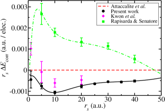
Figure 2: (Color online) Correlation energy of a paramagnetic Fermi fluid relative to the results of Attaccalite et al.attaccalite The results obtained by Kwon et al.kwon  and Rapisarda and Senatorerapisarda are shown for comparison. The results of Tanatar and Ceperleytanatar are not shown, because they are systematically too low in energy.kwon

Unlike Attaccalite et al.,attaccalite we fit Eq. (7) to paramagnetic data only; we do not attempt to calculate the spin-polarization-dependence of the energy of the HEG.

III.2 MD’s

The MD’s of paramagnetic HEG’s are shown in Fig. 3, and a more detailed graph of the MD at $r_{s}=5$ a.u. is shown in Fig. 4. The upper panel of Fig. 4 demonstrates that the extrapolated estimate is accurate and that the DMC results are converged with respect to the time step. It is clear from the lower panel of Fig. 4 that, although backflow makes a significant improvement to the QMC energy estimates, it has very little effect on the MD. The inclusion of backflow results in a small transfer of weight to wavevectors above the Fermi edge, as expected, because a greater fraction of correlation energy is retrieved. It can also be seen that the MD’s obtained at different system sizes are in agreement. We have therefore plotted data obtained at different system sizes together in Fig. 3. To our knowledge, the only previous QMC studies of the MD of the 2D HEG are those of Tanatar and Ceperleytanatar and Conti.conti At $r_{s}=10$ a.u., Tanatar and Ceperley found that the MD at small wave vectors is lower than the value near the Fermi edge. Our data do not show this unusual feature. Tanatar and Ceperley used a relatively inflexible Slater-Jastrow wave function, which may be the reason for the discrepancy. Giuliani and Vignalegiuliani quote a formula for the MD, which was obtained by fitting to QMC data generated by Conti.conti We have fitted our MD’s to a simplified version of the form suggested in Ref. giuliani, :

$$\rho=\frac{1}{2}\left\{\begin{array}[]{lr}a_{0}+a_{1}x+a_{2}x^{2}+a_{3}x^{3}+a_{4}x^{4}&~{}~{}~{}{\rm if}~{}x<\sqrt{2}\\ \frac{4g(0)r_{s}^{2}}{x^{6}}+\left(a_{7}+a_{8}x+a_{9}x^{2}\right)\exp\left[-\frac{\left(x-\sqrt{2}\right)^{2}}{a_{6}^{2}}\right]&{\rm if}~{}x>\sqrt{2}\end{array}\right.,$$ (8)

where $x=r_{s}k$ and the $a_{i}$ are fitting parameters. $g(0)$ is the contact PCF, which we evaluated using Eq. (9). The fitted parameters are given in Table 4. Our values for the discontinuity at the Fermi edge are slightly smaller than those reported in Ref. giuliani, .

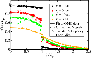
Figure 3: (Color online) Extrapolated MD $\rho(k)$ for paramagnetic Fermi fluids. $k_{\rm F}=\sqrt{2}/r_{s}$ is the Fermi wave vector of the paramagnetic fluid and $\rho_{\rm F}=r_{s}^{2}/(2\pi)$ is the value of the Fermi distribution. The results were obtained using a Slater-Jastrow-backflow wave function and a variety of system sizes with $N\geq 50$ in each case. Twist averaging was not used. For comparison, we have plotted the MD obtained by Tanatar and Ceperleytanatar (open symbols) and Eq. (8.133) of Ref. giuliani, (dotted lines).

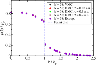
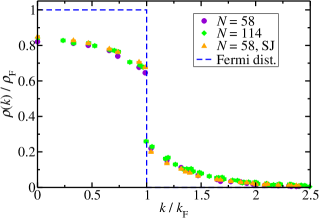
Figure 4: (Color online) MD $\rho(k)$ for paramagnetic Fermi fluids at $r_{s}=5$ a.u., obtained using VMC and DMC at different system sizes $N$. Backflow was used, except for the data labeled “SJ.” The upper panel shows the results obtained at $N=58$ using VMC and DMC with different time steps $\tau$. The lower panel shows the effect of changing the system size and using backflow on the extrapolated MD. Twist averaging was not used. $k_{\rm F}=\sqrt{2}/r_{s}$ is the Fermi wave vector of the paramagnetic fluid and $\rho_{\rm F}=r_{s}^{2}/(2\pi)$ is the value of the Fermi distribution.

$r_{s}$ (a.u.)	1		5		10		30
$a_{0}$	$1$.	$950$	$1$.	$649$	$1$.	$410$	$0$.	$974\,5$
$a_{1}$	$-0$.	$073\,42$	$-0$.	$038\,99$	$0$.	$336\,6$	$-0$.	$053\,5$
$a_{2}$	$0$.	$280\,5$	$0$.	$074\,18$	$-1$.	$199$	$0$.	$150\,9$
$a_{3}$	$-0$.	$388\,4$	$-0$.	$192\,0$	$1$.	$148$	$-0$.	$388\,8$
$a_{4}$	$0$.	$136\,5$	$0$.	$021\,98$	$-0$.	$436\,3$	$0$.	$147\,3$
$a_{6}$	$1$.	$171$	$1$.	$017$	$1$.	$035$	$1$.	$379$
$a_{7}$	$0$.	$164\,8$	$1$.	$682$	$2$.	$091$	$1$.	$428$
$a_{8}$	$-0$.	$113\,5$	$-1$.	$282$	$-1$.	$566$	$-0$.	$826\,4$
$a_{9}$	$0$.	$021\,19$	$0$.	$277\,3$	$0$.	$343\,8$	$0$.	$159\,9$
$Z$	$0$.	$866$	$0$.	$398$	$0$.	$209$	$0$.	$055\,5$

Table 4: Fitting parameters in Eq. (8) for the MD and discontinuity $Z$ in the MD at the Fermi edge. The MD is normalized such that the Fermi distribution is 1.

III.3 SSF’s

VMC and DMC SSF’s of a 50-electron paramagnetic HEG at $r_{s}=1$ a.u. are shown in Fig. 5. It can be seen that the difference between the VMC and DMC data is in most cases smaller than the difference between the two sets of DMC data, implying that the errors due to extrapolated estimation are small. On the other hand, the difference between the data with ${\bf k}_{s}={\bf 0}$ and the twist-averaged data is significant. In particular, the former has some unusual features close to integer multiples of the Fermi wave vector, one of which is shown in the inset to Fig. 5. Elsewhere, twist averaging has only a small effect. At all densities we find that the twist-averaged SSF in a 50- or 58-electron cell is in agreement with the SSF in a 114-electron cell, as can be seen in Fig. 5. Since the statistical errors are less significant at the smaller system sizes, we have used $N=50$ or 58 electrons in the high-density data reported below.

The SSF’s of paramagnetic and ferromagnetic fluids at low density are shown in Fig. 6, while the SSF’s of paramagnetic fluids at high density are shown in Fig. 7. It can be seen that a peak in the SSF at about $k=2.62k_{\rm F}$ appears at low density, perhaps due to incipient Wigner crystallization. Our SSF’s are in good agreement with those of Gori-Giorgi et al.gorigiorgi_pcf

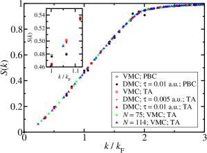
Figure 5: (Color online) SSF $S(k)$ for a paramagnetic HEG of density parameter $r_{s}=1$ a.u. $k_{\rm F}=\sqrt{2}/r_{s}$ is the Fermi wave vector of the paramagnetic fluid. The system size was $N=50$ electrons, except where indicated otherwise. Results obtained with ${\bf k}_{s}={\bf 0}$ (“PBC”) and twist averaging (“TA”) are shown. A Slater-Jastrow-backflow wave function was used in each case. The inset shows in greater detail one of the regions in which the twist-averaged and non-twist-averaged data disagree.

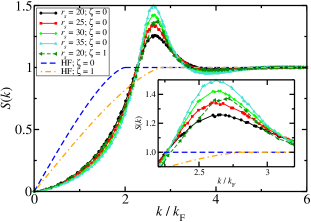
Figure 6: (Color online) Extrapolated SSF $S(k)$ for HEG’s of density parameter $r_{s}$ and spin polarization $\zeta$. $k_{\rm F}=\sqrt{2}/r_{s}$ is the Fermi wave vector of the paramagnetic fluid. The results were obtained using a Slater-Jastrow-backflow wave function and twist averaging. System sizes of $N=90$, 114, 90, and 114 were used in the paramagnetic calculations at $r_{s}=20$, 25, 30, and 35 a.u., respectively, and a system size of $N=45$ was used in the ferromagnetic calculation at $r_{s}=20$ a.u. The inset shows the peak in greater detail.

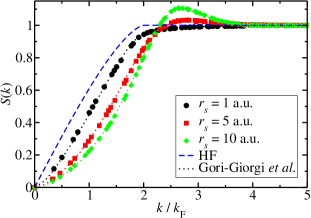
Figure 7: (Color online) Extrapolated SSF $S(k)$ for paramagnetic HEG’s at high density. $k_{\rm F}=\sqrt{2}/r_{s}$ is the Fermi wave vector. Slater-Jastrow-backflow wave functions and twist averaging were used. The system sizes are $N=50$, 58, and 58 at $r_{s}=1$, 5, and 10 a.u., respectively. The curve marked “HF” shows the Hartree-Fock SSF. The dotted lines show the SSF obtained by taking the Fourier transform of the PCF data of Gori-Giorgi et al.gorigiorgi_pcf

III.4 PCF’s

We compare PCF’s obtained at different system sizes using different QMC methods for a paramagnetic HEG at $r_{s}=5$ a.u. in Fig. 8. The difference between the VMC and DMC PCF’s, and the difference between extrapolated PCF’s obtained with and without backflow is small, implying that the error in the extrapolated PCF is small. Twist averaging has a small effect on the PCF, but the twist-averaged PCF’s at $N=58$ and $N=114$ electrons are very similar, implying that the finite-size error in the twist-averaged PCF at $N=58$ is small. We have also verified that the PCF is converged with respect to the DMC time step.

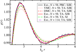
Figure 8: (Color online) VMC, DMC, and extrapolated (“Ext.”) PCF’s $g(r)$ for a paramagnetic Fermi fluid of density parameter $r_{s}=5$ a.u. at different system sizes $N$. Twist averaging was used in the curves labeled “TA,” but not in the one labeled “PBC.” Slater-Jastrow and Slater-Jastrow-backflow wave functions were used in the curves labeled “SJ” and “SJB,” respectively. $k_{\rm F}=\sqrt{2}/r_{s}$ is the Fermi wave vector of the paramagnetic fluid.

Our PCF’s are shown in Figs. 9 (high density) and 10 (low density), along with the results of Gori-Giorgi et al.gorigiorgi_pcf Our PCF’s are in good agreement with those of Gori-Giorgi et al. (as expected, from the SSF results in Fig. 7).

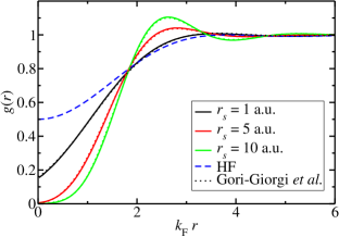
Figure 9: (Color online) Extrapolated total PCF $g(r)$ for paramagnetic Fermi fluids of density parameter $r_{s}$. $k_{\rm F}=\sqrt{2}/r_{s}$ is the Fermi wave vector of the paramagnetic fluid. “HF” stands for Hartree-Fock theory. Twist averaging was used and the QMC calculations were performed at system sizes of $N=50$, 58, and 58 electrons at $r_{s}=1$, 5, and 10 a.u. The dotted lines show the data of Gori-Giorgi et al.,gorigiorgi_pcf which are almost indistinguishable from our data.

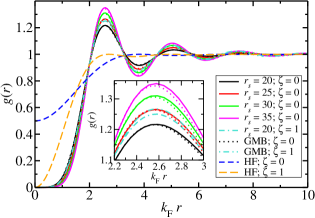
Figure 10: (Color online) Extrapolated total PCF $g(r)$ for Fermi fluids of density parameter $r_{s}$ and spin polarization $\zeta$. $k_{\rm F}=\sqrt{2}/r_{s}$ is the Fermi wave vector of the paramagnetic fluid. “GMB” denotes the work of Gori-Giorgi et al.gorigiorgi_pcf  (shown by dotted lines), while “HF” stands for Hartree-Fock theory. Twist averaging was used and the QMC calculations were performed at system sizes of $N=90$, 114, 90, and 114 at $r_{s}=20$, 25, 30, and 35, respectively.

The contact PCF $g(0)$ is especially important in the construction of generalized-gradient-approximation exchange-correlation functionals.giuliani We give our $g(0)$ values in Table 5, and we plot $r_{s}g(0)$ against $r_{s}$ in Fig. 11, along with some other results in the literature. Because our PCF’s have converged with respect to system size, and our VMC and DMC results agree with each other when backflow is used, we have simply averaged our VMC and DMC $g(0)$ data at different system sizes in order to reduce the statistical noise in our estimate of the contact PCF. Our results are in reasonably good agreement with the fit to the earlier QMC data of Gori-Giorgi et al.gorigiorgi_pcf and also with the expression for $g(0)$ obtained using ladder theory by Nagano et al.nagano Interestingly, our results clearly disagree with the more recent calculation of $g(0)$ within ladder theory by Qian,qian which involved fewer approximations than the work of Nagano et al. The close agreement between our results and those of Nagano et al. must therefore be regarded as a coincidence. The fact that our QMC calculations, using a different trial wave function, are consistent with the data of Gori-Giorgi et al. strongly suggests that the QMC results for $g(0)$ are reliable, whereas ladder theory is of limited use at low densities. Our results are also in clear disagreement with the formula proposed by Polini et al.,polini which interpolates between the results of ladder theory at high-density (where it should be exact) and a partial-wave analysis at low density.

$r_{s}$ (a.u.)	$g(0)$
1	$0$.	$151\,7(4)$
3	$0$.	$022\,7(2)$
5	$0$.	$005\,0(3)$
7	$0$.	$001\,25(5)$
10	$0$.	$000\,24(2)$

Table 5: Contact PCF of paramagnetic HEG’s at five different densities. Twist-averaged VMC and DMC results obtained at different system sizes were averaged to obtain these data.

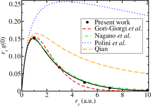
Figure 11: (Color online) Contact PCF $g(0)$ against density parameter $r_{s}$, as calculated by different authors: the present work (see Table 5), Gori-Giorgi et al.,gorigiorgi_pcf Nagano et al.,nagano Polini et al.,polini and Qian.qian

The fit to our $g(0)$ data shown in Fig. 11 is

$$g(0)=\frac{1}{2}\left\{\begin{array}[]{lr}\left(1+Ar_{s}+Br_{s}^{2}\right)\exp(-Er_{s})&r_{s}\geq 1\\ 1+ar_{s}+br_{s}^{2}+cr_{s}^{3}&r_{s}<1\end{array}\right.,$$ (9)

where $A=-0.25724$, $B=0.071116$, and $E=0.98553$ were obtained by fitting. Polini et al.polini  have shown that $\lim_{r_{s}\rightarrow 0}g(0)=(1/2)[1-1.372r_{s}]$, so we have set $a=-1.372$ and determined $b=0.997618888$ and $c=-0.3218467056$ by matching the value and derivative of $g(0)$ at $r_{s}=1$ a.u.footnote:g0_fit

IV Conclusions

We have studied the ground-state properties of the fluid phases of the 2D HEG using QMC. We used highly accurate trial wave functions and dealt with finite-size effects by twist averaging. Twist averaging removes some strange features in the SSF, but our PCF’s and SSF’s are in good agreement with analytic fits to earlier QMC data,gorigiorgi_pcf confirming the accuracy of these formulas. Our MD’s show some qualitative differences from earlier QMC results,tanatar however; in particular, we do not observe an increase in the MD as the Fermi edge is approached at low density. Finally, we have reported DMC energy data for the high-density 2D HEG, which we used to construct a new exchange-correlation functional for 2D DFT calculations.

V Acknowledgments

We acknowledge financial support from Jesus College, Cambridge and the UK Engineering and Physical Sciences Research Council (EPSRC). Computing resources were provided by the Cambridge High Performance Computing Service and HPCx.

References

- (1) D. M. Ceperley and B. J. Alder, Phys. Rev. Lett. 45, 566 (1980).
- (2) W. M. C. Foulkes, L. Mitas, R. J. Needs, and G. Rajagopal, Rev. Mod. Phys. 73, 33 (2001).
- (3) B. Tanatar and D. M. Ceperley, Phys. Rev. B 39, 5005 (1989).
- (4) F. Rapisarda and G. Senatore, Aust. J. Phys. 49, 161 (1996).
- (5) N. D. Drummond and R. J. Needs, unpublished (2008).
- (6) Y. Kwon, D. M. Ceperley, and R. M. Martin, Phys. Rev. B 58, 6800 (1998).
- (7) P. Gori-Giorgi, S. Moroni, and G. B. Bachelet, Phys. Rev. B 70, 115102 (2004).
- (8) Z. Qian, Phys. Rev. B 73, 035106 (2006).
- (9) S. Conti, PhD thesis, Scuola Normale Superiore, Pisa (1997).
- (10) G. F. Giuliani and G. Vignale, Quantum Theory of the Electron Liquid, Cambridge University Press, Cambridge (2005); Errata: http://www.missouri.edu/physvign/errata.pdf.
- (11) R. J. Needs, M. D. Towler, N. D. Drummond, and P. López Ríos, CASINO version 2.1 User Manual, University of Cambridge, Cambridge (2008).
- (12) J. B. Anderson, J. Chem. Phys. 65, 4121 (1976).
- (13) N. D. Drummond, M. D. Towler, and R. J. Needs, Phys. Rev. B 70, 235119 (2004).
- (14) P. López Ríos, A. Ma, N. D. Drummond, M. D. Towler, and R. J. Needs, Phys. Rev. E 74, 066701 (2006).
- (15) C. J. Umrigar, K. G. Wilson, and J. W. Wilkins, Phys. Rev. Lett. 60, 1719 (1988).
- (16) N. D. Drummond and R. J. Needs, Phys. Rev. B 72, 085124 (2005).
- (17) C. J. Umrigar, J. Toulouse, C. Filippi, S. Sorella, and R. G. Hennig, Phys. Rev. Lett. 98, 110201 (2007).
- (18) G. Rajagopal, R. J. Needs, S. Kenny, W. M. C. Foulkes, and A. James, Phys. Rev. Lett. 73, 1959 (1994); G. Rajagopal, R. J. Needs, A. James, S. D. Kenny, and W. M. C. Foulkes, Phys. Rev. B 51, 10591 (1995).
- (19) Y. Kwon, D. M. Ceperley, and R. M. Martin, Phys. Rev. B 48, 12037 (1993).
- (20) C. Lin, F. H. Zong, and D. M. Ceperley, Phys. Rev. E 64, 016702 (2001).
- (21) C. Attaccalite, S. Moroni, P. Gori-Giorgi, and G. B. Bachelet, Phys. Rev. Lett. 88, 256601 (2002); C. Attaccalite, S. Moroni, P. Gori-Giorgi, and G. B. Bachelet, Phys. Rev. Lett. 91, 109902(E) (2003).
- (22) S. Baroni and S. Moroni, Phys. Rev. Lett. 82, 4745 (1999).
- (23) N. D. Drummond, R. J. Needs, A. Sorouri, and W. M. C. Foulkes, Phys. Rev. B 78, 125106 (2008).
- (24) S. Nagano, K. S. Singwi, and S. Ohnishi, Phys. Rev. B 29, 1209 (1984); S. Nagano, K. S. Singwi, and S. Ohnishi, Phys. Rev. B 31, 3166 (1985).
- (25) M. Polini, G. Sica, B. Davoudi, and M. P. Tosi, J. Phys.: Condens. Matter 13, 3591 (2001).
- (26) One can satisfy by imposing in Eq. (9); however, we found the corresponding fits to be poor, because it is inappropriate to use the high-density expansion to determine the exponent which controls how rapidly falls off at low density.