An exact expression for the Reynolds number dependence of the energy dissipation rate in homogeneous, isotropic turbulence

Abstract

The Reynolds number dependence of the dimensionless dissipation rate $C_{\varepsilon}=\varepsilon L/U^{3}$ is derived directly from the Karman-Howarth equation as $C_{\varepsilon}=C_{\varepsilon,\infty}[1+A/R_{L}]$, where the coefficient $A$ depends on the second- and third-order structure functions, $R_{L}=UL/\nu$, $L$ is the integral length scale, and $U$ is the rms velocity. Fitting this form to results from DNS indicates that $A$ is effectively constant and hence the predicted dependence of $C_{\varepsilon}$ on Reynolds number is as $R_{L}^{-1}$.

PACS 47.27.Ak, 47.27.E-

In recent years, there has been great interest in the Reynolds number dependence of the dissipation rate in homogeneous, isotropic fluid turbulence: see [1]-[11]. Apart from its intrinsic fundamental interest, this is a key factor in the free decay of turbulence, which is one of the most studied aspects of the turbulence problem: see, for example, [12]-[15], and the many references therein.

We consider the dimensionless dissipation rate

$$\varepsilon=C_{\varepsilon}U^{3}/L,$$ (1)

which was put forward in 1935 by Taylor [16] on the basis of dimensional arguments. Here $U$ is the rms velocity of the fluid and $L$ is the integral length scale. As early as 1953, Batchelor [17] (in the first edition of this book) presented evidence to suggest that $C_{\varepsilon}$ tends to a constant with increasing Reynolds number. However, the present interest in the subject stems from the seminal paper by Sreenivasan [1], who established that in grid turbulence $C_{\varepsilon}$ became constant for Taylor-Reynolds numbers greater than about 50 but observed that the actual value could depend on the flow configuration and initial conditions.

Attempts have been made to establish a theoretical relationship between the dissipation rate and the Reynolds number. Lohse [18] used a mean-field closure of the Karman-Howarth equation to obtain an approximate form, whereas Doering and Foias [19] have established upper and lower bounds to be satisfied by such relationships. In this Letter, we derive a new and exact relationship between the dissipation and the Reynolds number. We begin by stating the Karman-Howarth equation and reviewing the relevant phenomenology.

As is well known, the Karman-Howarth equation [20] is derived directly from the Navier-Stokes equation and is an exact relationship expressing conservation of energy. It may be written in terms of structure functions as [21]:

$$-\frac{2}{3}\varepsilon-\frac{1}{2}\frac{\partial S_{2}}{\partial t}=\frac{1}{6r^{4}}\frac{\partial}{\partial r}(r^{4}S_{3})-\frac{\nu}{r^{4}}\frac{\partial}{\partial r}\left(r^{4}\frac{\partial S_{2}}{\partial r}\right),$$ (2)

where the structure function of order $n$ is given by

$$S_{n}=\left\langle\left(u(r)-u(0)\right)^{n}\right\rangle.$$ (3)

We begin by re-writing it as an expression for the dissipation rate, thus:

$$\varepsilon=-\frac{3}{4}\frac{\partial S_{2}}{\partial t}-\frac{1}{4r^{4}}\frac{\partial}{\partial r}(r^{4}S_{3})+\frac{3\nu}{2r^{4}}\frac{\partial}{\partial r}\left(r^{4}\frac{\partial S_{2}}{\partial r}\right).$$ (4)

Now we re-visit the Richardson-Kolmogorov phenomenology of this equation [17], as this will be of specific use to us later on. We first consider the stationary case and, as usual, this requires the injection of energy at scales $r\geq r_{I}$ (say). As the Karman-Howarth equation is local in $r$, we restrict our attention to scales less than the injection scale $r_{I}$ and set the time-derivative equal to zero. With these steps, equation (4) becomes:

$$\varepsilon=-\frac{1}{4r^{4}}\frac{\partial}{\partial r}(r^{4}S_{3})+\frac{3\nu}{2r^{4}}\frac{\partial}{\partial r}\left(r^{4}\frac{\partial S_{2}}{\partial r}\right).$$ (5)

We note that each term on the right hand side is separately a function of $r$ but that jointly they are constant, as required to match the dissipation rate on the left hand side. If we go further, and restrict the values of the scale to $r\geq r_{d}$, where $r_{d}$ is the dissipation lengthscale, then for sufficiently large values of the Reynolds number the well known arguments of Kolmogorov (K41) [22, 23] apply. In order to apply this rigorously, we take the infinite Reynolds number limit. This means taking the limit $\nu\rightarrow 0$ such that $\varepsilon$ remains constant [17]. The viscous term may then be set equal to zero, and the remaining term on the right hand side represents the inertial flux of energy, which is now constant, and equal to the dissipation rate. Hence:

$$\varepsilon=-\frac{1}{4r^{4}}\frac{\partial}{\partial r}(r^{4}S_{3}).$$ (6)

From this equation it is a simple matter to recover Kolmogorov’s famous ‘4/5’ law for the third-order structure function, thus:

$$S_{3}(r)=-\frac{4}{5}\varepsilon r.$$ (7)

Next we make a change of variables based on constant velocity- and length-scales, $V$ and $l$, respectively. As an example, we will put the second-order structure function into a dimensionless form. We do this by expanding $S_{2}$ in a Taylor-Maclaurin series. Note that this is a general operation and is not restricted to any particular values of $r$. Then, introducing a dimensionless variable $x$, through $r=lx$, we have

$$S_{2}(r) = S_{2}(0)+S^{\prime}_{2}(0)r+\frac{1}{2}S_{2}^{\prime\prime}(0)r^{2}+\dots,$$ (8)

$$= S_{2}(0)+S^{\prime}_{2}(0)lx+\frac{1}{2}S_{2}^{\prime\prime}(0)l^{2}x^{2}+\dots,$$

$$= V^{2}\left[f_{2}(0)+f^{\prime}_{2}(0)x+\frac{1}{2}f_{2}^{\prime\prime}(0)x^{2}+\dots\right],$$

$$\equiv V^{2}f_{2}(x),$$

where, in the third line, we have renamed coefficients in order to extract a factor $V^{2}$, and also to absorb powers of $l$. Note that the primes denote differentiation with respect to $r$ in the first two lines but with respect to $x$ in the third. Lastly, we have defined the dimensionless second-order structure function $f_{2}(x)$ as the sum of the Maclaurin series in the new coefficients.

We can repeat this process for structure functions of any order $n$, and we summarise the general result as:

$$S_{n}=V^{n}f_{n}(x),\qquad\mbox{with}\qquad x=\frac{r}{l}.$$ (9)

We should note that this procedure involves no approximations or non-trivial assumptions. It merely introduces the $f_{n}$ as dimensionless forms of the structure functions. As they are dimensionless, their dependence on $r$ must be scaled by some length, here denoted by $l$.

Then we make the specific choices $V=U$, the root-mean-square velocity, and $l=L$, the integral length scale. With these choices, and substituting from (9), we change equation (5) to the form:

$$\varepsilon=\frac{A_{3}U^{3}}{L}+\frac{A_{2}\nu U^{2}}{L^{2}},$$ (10)

where the coefficients $A_{3}$ and $A_{2}$ are given by

$$A_{3}\equiv-\frac{1}{4x^{4}}\frac{\partial}{\partial x}\left[x^{4}f_{3}(x)\right],$$ (11)

and

$$A_{2}\equiv\frac{3}{2x^{4}}\frac{\partial}{\partial x}\left[x^{4}\frac{\partial f_{2}}{\partial x}\right].$$ (12)

Then, if we divide both sides of (10) by $U^{3}/L$ we may write this as

$$C_{\varepsilon}=A_{3}+\frac{A_{2}}{R_{L}}=A_{3}\left[1+\frac{A_{2}}{A_{3}R_{L}}\right],$$ (13)

where the dimensionless dissipation $C_{\varepsilon}$ is as defined in (1) and the Reynolds number is given by $R_{L}=UL/\nu$. Note that the $f_{n}$ are determined by (9), along with this choice of scaling variables, and hence so also are the coefficients $A_{3}$ and $A_{2}$. We also note that this equation is still just the Karman-Howarth equation: no approximation has been made.

Let us consider the asymptotic behaviour of this expression for large Reynolds numbers. In general the coefficients $A_{2}$ and $A_{3}$ may depend on the Reynolds number (although, as we shall see later, comparison with the results from DNS suggests that they are essentially constant, albeit with possibly some dependence on initial conditions). However, the asymptotic properties of (13) must be those of the Karman-Howarth equation. So taking the limit of infinite Reynolds numbers, and comparing (13) with (5), we note that the coefficient $A_{3}$ becomes constant, while the term $A_{2}/R_{L}$ vanishes. Then we obtain, by analogy with (6), the asymptotic form of (13) as

$$\lim_{R_{L}\rightarrow\infty}C_{\varepsilon}\equiv C_{\varepsilon,\infty}=A_{3}.$$ (14)

Substituting back into (13) then yields

$$C_{\varepsilon}=C_{\varepsilon,\infty}\left[1+A/R_{L}\right],$$ (15)

where

$$A=A_{2}/A_{3}.$$ (16)

We now discuss the extension of our results to freely decaying isotropic turbulence. Of course, the neglect of the time-derivative term in (2) is quite usual, even for decaying turbulence, provided that the Reynolds number is large enough and that one restricts attention to the inertial range. For instance, this step is required in order to derive the ‘4/5’ law for decaying turbulence and is known as local stationarity. However, we wish to consider a more general approach in which we introduce the time dependence of all statistical quantities, so that we now have $\varepsilon(t)$ and $S_{n}(r,t)$, at any time $t$.

In order to make comparisons with the stationary case, we take some fiducial time $t=t_{e}$, when the turbulence is assumed to have evolved from arbitrary initial conditions to a state determined solely by the Navier-Stokes equations. Then, as before, we introduce a change of variables, such that

$$S_{n}(r,t)=U^{n}(t_{e})g_{n}(x,\tau),$$ (17)

where now

$$x=r/L(t_{e});\qquad\tau=t/T;\qquad T=L(t_{e})/U(t_{e}).$$ (18)

Just as before, in the stationary case, the introduction of the dimensionless (but now time-dependent) structure functions $g_{n}(x,\tau)$ may be accomplished by the use of Taylor series; although, in this case, it is for a function of two variables.

It should be emphasised that the form (17) is not a similarity solution of any kind. If we were to drop the dependence on the variable $\tau$ then this would amount to an assumption of self-preservation, as introduced by von Karman in 1938 [20]. However, this is one of the vexed issues of turbulence theory. It runs into difficulties, not least because during free decay the characteristic length changes from the integral length scale to the viscous scale in the final period of the decay: see, for instance, [13]. As it is, we reiterate that we do not make any such assumption and that we retain the full time dependence of the problem.

With this in mind, it is easily shown that substituting (17) into (4) leads to a generalization of equation (13) to the form:

$$C_{\varepsilon}=(A_{3}-B_{2})\left[1+\frac{1}{R_{L}}\frac{A_{2}}{A_{3}-B_{2}}\right],$$ (19)

where the coefficients $A_{2}$ and $A_{3}$ are still defined by equations (12) and (11), but now with $f$ replaced by $g$, and the new coefficient $B_{2}$ is given by

$$B_{2}\equiv\left.\frac{3}{4}\frac{\partial g_{2}}{\partial\tau}\right|_{\tau_{e}}.$$ (20)

Let us now consider the effect of including this time dependence. We introduce the inertial flux which we denote by $\Pi_{max}$. (Formally, this quantity is defined in wavenumber space and for our present purposes we are interested in its maximum value with respect to wavenumber: for a discussion see [24].) Then, as is well known, for increasing Reynolds number, the maximum flux approaches the dissipation rate from below; or:

$$\lim_{R_{L}\rightarrow\infty}\Pi_{max}\rightarrow\varepsilon,$$ (21)

for stationary turbulence. Our present analysis indicates that this cannot, in principle, be the case for freely decaying turbulence.

We may see this as follows. Rewriting the coefficient $B_{2}$ in terms of the structure function, we have

$$B_{2}=\left.\frac{3}{4}\frac{\partial g_{2}}{\partial\tau}\right|_{\tau_{e}}=\left.\frac{3}{4}\frac{L(t_{e})}{U^{3}(t_{e})}\frac{\partial S_{2}}{\partial t}\right|_{t_{e}}.$$ (22)

For free decay, this coefficient must be negative. Taking its modulus we have

$$\lim_{R_{L}\rightarrow\infty}\varepsilon\rightarrow\frac{U^{3}}{L}(A_{3}+|B_{2}|).$$ (23)

Thus, in freely decaying turbulence, we have

$$\lim_{R_{L}\rightarrow\infty}\frac{\Pi_{max}}{\varepsilon}\rightarrow\frac{A_{3}}{A_{3}+|B_{2}|}<1,$$ (24)

and so the inertial flux of energy never quite reaches the same value as the dissipation. This result has implications for the interpretation of the Kolmogorov (K41) picture, when a comparison is made of forced and decaying homogeneous, isotropic turbulence, and we shall investigate this further in future work.

For completeness, we now give the extension of equation (13) to the case of free decay, as:

$$C_{\varepsilon}=C_{\varepsilon,\infty}\left[1+A/R_{L}\right],$$ (25)

where the dimensionless dissipation at infinite Reynolds number and the coefficient $A$ are now given by

$$C_{\varepsilon,\infty}=A_{3}-B_{2}\quad\mbox{and}\quad A=A_{2}/(A_{3}-B_{2}).$$ (26)

We may compare our results to those of other theories. Lohse [18] used a mean-field approximation to the Karman-Howarth equation and obtained the asymptotic result $C_{\varepsilon,\infty}=(6/b)^{3/2}$, where $b$ is the prefactor in the Kolmogorov inertial-range form of the second-order structure function. This may be compared with our equation (14), which in contrast gives $C_{\varepsilon,\infty}=A_{3}$. This difference from our result is only to be expected because a closure invariably involves expressing $S_{3}$ in terms of $S_{2}$. (It should be emphasised that our remarks here have no implications for the validity or accuracy of Lohse’s approximation.)

It is also of interest to compare equation (10), which is an intermediate stage in our calculation, to the result for an upper bound on the dissipation as given by Doering and Foias [19]. This is featured in their abstract as

$$\varepsilon\leq c_{1}\nu\frac{U^{2}}{l^{2}}+c_{2}\frac{U^{3}}{l},$$

and corresponds to their equation (40). Here the coefficients $c_{1}$ and $c_{2}$ depend on the shape of the forcing function, while $l$ is its longest length-scale. Obviously this is quite different from our own result, where the corresponding parameters depend on the fluid turbulence and not on the forcing. Also, we have an equality, rather than an inequality. Nevertheless, it can easily be shown that the two results are equivalent and this will be presented later, in a fuller account of this work.

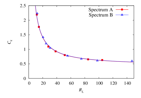
Figure 1: Values of $C_{\varepsilon}$ from DNS for two different initial spectra plotted against the integral length scale Reynolds number, $\mathcal{R}_{L}$. These points were fitted to the curve $y(x)=a+(b/x)$, as given by Eq. (25).

Lastly, we illustrate the dependence of the dissipation on Reynolds number by fitting the general form of equation (25) to the results of direct numerical simulations (DNS) of the Navier-Stokes equation. This is shown for two different initial spectra, which are generated using the following equation:

$$E(k,0)=C_{1}\mathrm{k}^{C_{2}}\exp\Big{\{}-C_{3}\mathrm{k}^{C_{4}}\Big{\}},$$ (27)

where the values taken for the parameters $C_{1}$-$C_{4}$ are as given in Table 1.

Initial spectra	$C_{1}$	$C_{2}$	$C_{3}$	$C_{4}$
Spectrum A	0.0017	4	0.08	2
Spectrum B	0.08	2	0.0824	2

Table 1: Initial energy spectra parameter values for use in the numerical computations. These parameters are substituted into Eq.(27) to generate the required initial spectrum.

Note that Spectrum A and Spectrum B have low-wavenumber regions varying as $k^{4}$ and $k^{2}$, respectively. The fitting process gives asymptotic values of $C_{\varepsilon,\infty}=0.43\pm 0.01$ and $C_{\varepsilon,\infty}=0.43\pm 0.02$, respectively.

Figure 1 illustrates the way in which our new exact relationship between the dimensionless dissipation rate and the Reynolds number can be used to fit the data generated by numerical or other experiments. In particular it supports the idea that the coefficient $A$ is constant with respect to the Reynolds number, even at low Reynolds numbers.

Summing up, we have taken the Karman-Howarth equation as an expression for the dissipation rate and transformed it into a more useful form, by making a change of variables. Then we have used its known properties to identifiy the asymptotic dimensionless dissipation coefficient and put it into the yet more useful form of (15). At no time have we made any approximation or similarity assumption. Our only mathematical assumption is the underlying one of theoretical physics: that all variables corresponding to physical observables are mathematically well-behaved. From our comparison with DNS, we conclude that the low-Reynolds number dependence of the dissipation coefficient is of the form: $\mbox{constant}\times R_{L}^{-1}$.

Currently we are working to extend the simulations to forced turbulence, in order to study the stationary case. In particular, we intend to study the detailed behaviour of the coefficients at small Reynolds numbers, including the extent of their dependence on the initial conditions. This work will be the subject of a full report in due course.

AB and SY were funded by the STFC, while WDM wishes to acknowledge the support provided by the award of an Emeritus Fellowship by the Leverhulme Trust, along with the hospitality of the Isaac Newton Institute (in the form of a Visiting Fellowship) and that of the Institute for Mathematical Sciences, Imperial College. He would also like to thank Francis Barnes, Claude Cambon, Stuart Coleman, Gregory Falkovich, Jorgen Frederiksen, Katepalli R. Sreenivasan, and Christos Vassilicos for stimulating discussions, helpful comments or other assistance.

References

- [1] K. R. Sreenivasan. Phys. Fluids, 27:1048, 1984.
- [2] K. R. Sreenivasan. Phys. Fluids, 10:528, 1998.
- [3] Y. Kaneda, T. Ishihara, M. Yokokawa, K. Itakura, and A. Uno. Phys. Fluids, 15:L21, 2003.
- [4] P. Burattini, P. Lavoie, and R. Antonia. Phys. Fluids, 17:098103, 2005.
- [5] B. R. Pearson, P.A Krogstad, and W. van de Water. Phys. Fluids, 14:1288, 2002.
- [6] B. R. Pearson, T. A. Yousef, N. E. L. Haugen A. Brandenburg, and P.A Krogstad. Phys. Rev. E, 70:056301, 2004.
- [7] D. A. Donzis, K. R. Sreenivasan, and P. K. Yeung. J. Fluid Mech., 532:199–216, 2005.
- [8] R. E. Seoud and J. C. Vassilicos. Physics of Fluids, 19:105108, 2007.
- [9] W. J. T. Bos, L. Shao, and J.-P. Bertoglio. Phys. Fluids, 19:045101, 2007.
- [10] N. Mazellier and J. C. Vassilicos. Phys. Fluids, 20:015101, 2008.
- [11] S. Goto and J. C. Vassilicos. Phys. Fluids, 21:035104, 2009.
- [12] W. K. George. Phys. Fluids A, 4:1492, 1992.
- [13] C. S. Speziale and P. S. Bernard. J. Fluid Mech., 241:645, 1992.
- [14] L. Skrbek and S. R. Stalp. Physics of Fluids, 12:1997, 2000.
- [15] H. Wang and W. K. George. J. Fluid Mech., 459:429, 2002.
- [16] G. I. Taylor. Proc. R. Soc., London, Ser. A, 151:421, 1935.
- [17] G.K. Batchelor. The theory of homogeneous turbulence. Cambridge University Press, Cambridge, 2nd edition, 1971.
- [18] Detlef Lohse. Phys. Rev. Lett., 73(22):3223 – 3226, 1994.
- [19] Charles R. Doering and Ciprian Foias. J. Fluid Mech., 467:289–306, 2002.
- [20] T. von Karman and L. Howarth. Proc. Roy. Soc. Lond. A, 164:192, 1938.
- [21] L. D. Landau and E. M. Lifshitz. Fluid Mechanics. Pergamon Press, London, English edition, 1959.
- [22] A. N. Kolmogorov. C. R. Acad. Sci. URSS, 30:301, 1941.
- [23] A. N. Kolmogorov. C. R. Acad. Sci. URSS, 32:16, 1941.
- [24] W. D. McComb. The Physics of Fluid Turbulence. Oxford University Press, 1990.