Gravitino Interactions from Yang-Mills Theory

Abstract

We fabricate gravitino vertex interactions using as only input on-shell Yang-Mills amplitudes and the Kawai-Lewellen-Tye gauge theory / gravity relations. A useful result of this analysis is simpler tree-level Feynman rules for gravitino scattering than in traditional gauges. All results are explicitly verified until five point scattering.

I Introduction

A remarkable and intimate connection between gravity and Yang-Mills amplitudes exist through the Kawai-Lewellen-Tye (KLT) relations Kawai:1985xq . In the field theory limit ($\alpha^{\prime}\rightarrow 0$) these relations take the form

$${\cal M_{\rm Gravity}}\sim\sum_{ij}K_{ij}{{\cal A}^{i\;L}_{\rm Yang-Mills}}\times{{{\cal A}^{j\;R}_{\rm Yang-Mills}}}\,.$$ (1)

Here $\mathcal{M}_{\rm Gravity}$, ${\cal A}^{i\;L}_{\rm Yang-Mills}$, ${\cal A}^{j\;R}_{\rm Yang-Mills}$ are gravity and Yang-Mills amplitudes and $K_{ij}$ is a specific function of kinematic invariants depending on the input Yang-Mills amplitudes. The KLT relations are a widely used tool for computing gravity amplitudes via a recycling of results for Yang-Mills amplitudes. For tree and loop amplitudes KLT can be combined with string theory inspired diagram rules as well as unitarity cut techniques Bern:1993wt ; BDDPR ; Bern:1999ji . Recently, inspired by Witten’s work WittenTopologicalString , we have seen remarkable progress in Yang-Mills amplitude computations (for recent reviews see Cachazo:2005ga ; Bern:2007dw ). Via KLT, this progress has fed into gravity yielding a much better understanding of amplitudes Giombi:2004ix ; Bern:2005bb ; BBSTgravity ; BDIgravity ; BjerrumBohr:2005jr ; BjerrumBohr:2006yw ; Benincasa:2007qj ; Bern:2007xj ; Ananth:2007zy ; Elvang:2007sg ; Hall:2008xn ; BjerrumBohr:2008vc ; ArkaniHamed:2008yf ; BjerrumBohr:2008ji ; Bern:2008qj ; ArkaniHamed ; Badger:2008rn ; Katsaroumpas:2009iy ; Bern:2006kd ; Cheung:2009dc ; BjerrumBohr:2009rd ; Stieberger:2009hq ; Boels:2009bv ; Chen:2010sr . It is now clear that gravity tree amplitudes have additional simplicity in their expressions. In many cases this simplicity appears very naturally from a string theory viewpoint BjerrumBohr:2008vc ; BjerrumBohr:2008ji ; ArkaniHamed ; Bern:2008qj ; Badger:2008rn ; BjerrumBohr:2009rd ; Stieberger:2009hq ; Chen:2010sr . Gravity loop amplitudes also have simple forms and one-loop amplitudes in ${\cal N}=8$ supergravity satisfy a ’no-triangle property’ Bern:2005bb ; BjerrumBohr:2006yw ; Bern:2007xj . This no-triangle property was first proven in BjerrumBohr:2008ji ; ArkaniHamed . No-triangle type of simplifications have been shown to hold even for pure gravity amplitudes Bern:2007xj ; BjerrumBohr:2008ji and also at the level of multi-loop amplitudes. Specifically, ${\cal N}=8$ supergravity amplitudes have been shown to satisfy very non-trivial cancellations at four-loop level Bern:2006kd (see also Green:2006gt ). Interestingly, KLT relations can be shown to hold regardless of the external matter content of the theory and in arbitrary dimension. KLT relations also hold for effective field theories of gravity Donoghue:1994dn ; Bern:1999bx ; EffKLT . We refer to ref. Bern:2002kj for a recent review and for further references on KLT and gravity amplitudes.

Although the KLT relations hold at the amplitude level in field theory, such relations have no natural framework at the Lagrangian level. It was however shown in a striking paper by Bern and Grant Bern:1999ji (see also Ananth:2007zy ) that one can construct graviton vertex interactions exclusively using the KLT relations as well as QCD gluon amplitudes as input. In this paper it is our aim to extend their analysis of graviton interactions to gravitinos and demonstrate how compact and factorized gravitino Feynman rules can be fabricated. As in the paper by Bern and Grant we will use the KLT relations together with amplitude expressions from Yang-Mills theory to derive results for vertex rules. As we are considering gravitino amplitudes we need to consider both gluon and fermion amplitudes. All results will be demonstrated to be consistent with those derived via traditional methods.

II Review of KLT relations

Tree amplitudes in gravity theories can be computed using the Einstein-Hilbert Lagrangian which is given by

$$\mathcal{L}=\frac{2}{\kappa^{2}}\sqrt{-g}R+{\cal L}_{\rm m}\,.$$ (2)

We employ conventional metric $(+1,-1,-1,-1)$ and define $\kappa=\sqrt{32\pi G}$. In the above equation $g$ denotes the determinant of the metric and $R$ is the Ricci scalar. The term ${\cal L}_{\rm m}$ contains possible matter interactions involving gravitons and other fields such as e.g. gravitinos. In order to derive vertex interactions one normally expands $g_{\mu\nu}$ around flat space, (i.e. $g_{\mu\nu}=\eta_{\mu\nu}+\kappa h_{\mu\nu}$), make a choice of gauge, and finally derive propagator and vertices from considering terms of order $\sim h^{2}$, $\sim h^{3}$, $\ldots$ and various matter couplings respectively.

In the text we will let $h$, $\widetilde{h}$, $g$ and $\widetilde{g}$ denote gravitons, gravitinos, gluons and gluinos. We will use the spinor helicity formalism wherever convenient. We define the antisymmetric tensor by $\epsilon^{0123}={+}1$ and $\gamma_{5}$ by $i\;\gamma_{0}\gamma_{1}\gamma_{2}\gamma_{3}$. All momenta in amplitudes are considered to be out-going. We will define

$$|p^{\pm}\rangle=u^{\pm}(p)=\frac{1}{2}(1\pm\gamma_{5})u(p),\ \ \ \langle p^{\pm}|=\bar{u}^{\pm}(p)=\bar{u}(p)\frac{1}{2}(1\mp\gamma_{5})\,,$$ (3)

where $\cancel{p}u(p)=0$ and $|p^{\pm}\rangle=C(\langle p^{\pm}|)^{T}$ and $C$ is the charge conjugation matrix ($C^{T}={-}C$, $C^{\dagger}C=1$, $C^{-1}\gamma_{\mu}C={-}\gamma^{T}_{\mu}$). Spinors are normalized so that

$$\langle p^{\pm}|\gamma^{\mu}|p^{\pm}\rangle=\bar{u}^{\pm}_{a}(p)\gamma^{\mu\,(ab)}u^{\pm}_{b}(p)=2p^{\mu}\,.$$ (4)

At times we will use shorthand notation such as

$$\langle AB\rangle=\langle p_{A}^{-}|p_{B}^{+}\rangle,\ \ \ [AB]=\langle p_{A}^{+}|p_{B}^{-}\rangle\,.$$ (5)

All spinor products are anti-symmetric so that $\langle AB\rangle=-\langle BA\rangle$ and they are all subject to the Schouten identities

$$\langle AB\rangle\langle CD\rangle+\langle AD\rangle\langle BC\rangle+\langle AC\rangle\langle DB\rangle=0\,.$$ (6)

We have $\langle p_{A}^{-}|\gamma^{\mu}|p_{B}^{-}\rangle=\langle p_{B}^{+}|\gamma^{\mu}|p_{A}^{+}\rangle\,,$ and (via a Fierz rearrangement)

$$\langle p_{A}^{+}|\gamma_{\mu}|p_{B}^{+}\rangle\langle p_{C}^{+}|\gamma^{\mu}|p_{D}^{+}\rangle=2[AC]\langle DB\rangle\,.$$ (7)

External gluinos can in the spinor helicity formalism be represented by either

$$\bar{\varepsilon}_{\widetilde{g}}^{\pm}(p)=\langle p^{\pm}|\ \ \ {\rm or}\ \ \ \varepsilon_{\widetilde{g}}^{\pm}(p)=|p^{\mp}\rangle\,.$$ (8)

Polarization vectors for gluons Xu:1986xb ; Mangano:1990by can be defined as

$$\varepsilon^{\pm\mu}_{g}(p,q)=\pm\frac{\langle p^{\pm}|\gamma^{\mu}|q^{\pm}\rangle}{\sqrt{2}\langle q^{\mp}|p^{\pm}\rangle}\,.$$ (9)

Here $q$ is a reference spinor (we will at times suppress the reference spinors in equations to avoid unnecessary cluttering of expressions). We will construct polarization tensors of the gravitino field via

$$\bar{\varepsilon}^{\pm\mu}_{\widetilde{h}}(p,q)=\bar{\varepsilon}_{\widetilde{g}}^{\pm}(p)\varepsilon^{\pm\mu}_{g}(p,q)\,,$$ (10)

while the polarization tensors of the graviton field will be given by

$$\varepsilon^{\pm\mu\nu}_{h}(p,q)=\varepsilon_{g}^{\pm\mu}(p,q)\varepsilon^{\pm\nu}_{g}(p,q)\,.$$ (11)

We will first consider more traditional ways of dealing with gravitino scattering (see e.g. Rarita:1941mf ; Freedman:1976xh ; Ferrara:1976ni ; Das:1976ct ; Grisaru:1976vm ; Grisaru:1977px ). Our starting point will be the following matter Lagrangian $({\cal L}_{\rm m})$

$$\begin{split}\mathcal{L}_{\rm m}=-\frac{1}{2}\epsilon^{\mu\nu\rho\sigma}\bar{\Psi}_{\mu}\gamma_{5}\gamma_{\nu}D_{\rho}\Psi_{\sigma}+\frac{\kappa^{2}\sqrt{-g}}{128}\big{(}2\bar{\Psi}_{\mu}\gamma_{\nu}\Psi_{\rho}\bar{\Psi}^{\nu}\gamma^{\mu}\Psi^{\rho}+\bar{\Psi}_{\mu}\gamma_{\nu}\Psi_{\rho}\bar{\Psi}^{\mu}\gamma^{\nu}\Psi^{\rho}-4\bar{\Psi}_{\mu}\gamma^{\mu}\Psi_{\rho}\bar{\Psi}_{\lambda}\gamma^{\lambda}\Psi^{\rho}\big{)}\,.\end{split}$$ (12)

This Lagrangian governs the spin-${3\over 2}$ gravitino field in curved space. The covariant derivative is defined via $D_{\rho}=\partial_{\rho}{+}\frac{1}{8}\omega_{\rho}^{\phantom{\rho}mn}[\gamma_{m},\gamma_{n}]$ and the spin connection $\omega_{\rho}^{\phantom{\rho}mn}$ is the usual one.

To make a traditional computation of amplitudes with external gravitinos, one can expand the kinetic part of the Lagrangian (here to lowest order in the graviton field). Discarding the antisymmetric vierbein field gives rise to the following Lagrangian

$$\begin{split}\mathcal{L}_{\rm m}&=-\frac{1}{2}\epsilon^{\mu\nu\rho\sigma}\bar{\Psi}_{\mu}\gamma_{5}\gamma_{\nu}\partial_{\rho}\Psi_{\sigma}-\frac{\kappa}{4}\epsilon^{\mu\nu\rho\sigma}\bar{\Psi}_{\mu}\gamma_{5}\gamma^{\alpha}h_{\alpha\nu}\partial_{\rho}\Psi_{\sigma}-\frac{\kappa}{16}\epsilon^{\mu\nu\rho\sigma}\bar{\Psi}_{\mu}\gamma_{5}\gamma_{\nu}[\gamma^{\alpha},\gamma^{\beta}]\Psi_{\sigma}\partial_{\beta}h_{\rho\alpha}\\ &\hskip 85.35826pt+\frac{\kappa^{2}}{128}\big{(}2\bar{\Psi}_{\mu}\gamma_{\nu}\Psi_{\rho}\bar{\Psi}^{\nu}\gamma^{\mu}\Psi^{\rho}+\bar{\Psi}_{\mu}\gamma_{\nu}\Psi_{\rho}\bar{\Psi}^{\mu}\gamma^{\nu}\Psi^{\rho}-4\bar{\Psi}_{\mu}\gamma^{\mu}\Psi_{\rho}\bar{\Psi}_{\lambda}\gamma^{\lambda}\Psi^{\rho}\big{)}\,.\end{split}$$ (13)

From this equation it is simple to find vertex factors Nielsen:1978ex ; Grisaru:1977zk . E.g. if we have two gravitinos with momentum $p^{\prime}$ and $p$ (Lorentz indices $\nu$ and $\mu$) and a graviton leg with momentum $q$ (Lorentz indices $\alpha,\beta$) we arrive at (all factors of the coupling constant $\frac{\kappa}{2}$ have been suppressed)

$$\begin{split}V_{\tilde{h}\tilde{h}h}^{\nu,\mu,\alpha\beta}(p^{\prime},p,q)&=-\frac{i}{2}\big{(}[\gamma^{\nu}\eta^{\mu\alpha}-\gamma^{\mu}\eta^{\nu\alpha}](p+p^{\prime})^{\beta}+[\cancel{p}-\cancel{p}^{\prime}]\eta^{\mu\nu}\eta^{\alpha\beta}+\gamma^{\alpha}(p-p^{\prime})^{\beta}\eta^{\mu\nu}\\ &\hskip 199.16928pt-2\gamma^{\alpha}\eta^{\mu\beta}p^{\nu}+2\gamma^{\alpha}\eta^{\nu\beta}p^{\prime\mu}\big{)}\,.\end{split}$$ (14)

III The Gravitino interactions from Yang-Mills theory

We will in this section use the KLT relations to construct (spin-${3\over 2}$) gravitino Feynman rules from Yang-Mills amplitudes involving gluons $g$ (spin-1) and gluinos $\widetilde{g}$ (spin-${1\over 2}$). KLT relations valid up till five points are e.g.:

$$\mathcal{M}_{3}{(1^{\sigma_{1}+\bar{\sigma}_{1}},2^{\sigma_{2}+\bar{\sigma}_{2}},3^{\sigma_{3}+\bar{\sigma}_{3}})}\;=\;i(-1)^{N_{p}+1}{\cal A}_{3}(1^{\sigma_{1}},2^{\sigma_{2}},3^{\sigma_{3}}){\cal A}_{3}(1^{\bar{\sigma}_{1}},2^{\bar{\sigma}_{2}},3^{\bar{\sigma}_{3}})\,,$$ (15)

$$\mathcal{M}_{4}(1^{\sigma_{1}+\bar{\sigma}_{1}},2^{\sigma_{2}+\bar{\sigma}_{2}},3^{\sigma_{3}+\bar{\sigma}_{3}},4^{\sigma_{4}+\bar{\sigma}_{4}})\;=\;i(-1)^{N_{p}+1}s_{12}{\cal A}_{4}(1^{\sigma_{1}},2^{\sigma_{2}},3^{\sigma_{3}},4^{\sigma_{4}}){\cal A}_{4}(1^{\bar{\sigma}_{1}},2^{\bar{\sigma}_{2}},4^{\bar{\sigma}_{4}},3^{\bar{\sigma}_{3}})\,,$$ (16)

$$\begin{split}\mathcal{M}_{5}(1^{\sigma_{1}+\bar{\sigma}_{1}},2^{\sigma_{2}+\bar{\sigma}_{2}},3^{\sigma_{3}+\bar{\sigma}_{3}},4^{\sigma_{4}+\bar{\sigma}_{4}},5^{\sigma_{5}+\bar{\sigma}_{5}})\;=\;\\ &i\big{[}s_{12}s_{34}(-1)^{N_{p}}{\cal A}_{5}(1^{\sigma_{1}},2^{\sigma_{2}},3^{\sigma_{3}},4^{\sigma_{4}},5^{\sigma_{5}}){\cal A}_{5}(2^{\bar{\sigma}_{2}},1^{\bar{\sigma}_{1}},4^{\bar{\sigma}_{4}},3^{\bar{\sigma}_{3}},5^{\bar{\sigma}_{5}})\\ &+s_{13}s_{24}(-1)^{N_{p}^{\prime}}{\cal A}_{5}(1^{\sigma_{1}},3^{\sigma_{3}},2^{\sigma_{2}},4^{\sigma_{4}},5^{\sigma_{5}}){\cal A}_{5}(3^{\bar{\sigma}_{3}},1^{\bar{\sigma}_{1}},4^{\bar{\sigma}_{4}},2^{\bar{\sigma}_{2}},5^{\bar{\sigma}_{5}})\big{]}\,.\end{split}$$ (17)

In these equations $N_{p}$ is a relative measure for the number of permutations of fermions on the right hand side of the equation as compared to the number of permutations on the left hand side, $s_{ij}=(p_{i}+p_{j})^{2}$ are generalized Mandelstam variables, $\mathcal{M}_{n}$ are gravity amplitudes (with suppressed coupling constants) and ${\cal A}_{n}$ are color-ordered amplitudes defined in terms of the full amplitude as in Mangano:1990by (see also Dixon:1996wi ). The propagators and vertex factors for color-ordered gluon/gluino diagrams are shown in fig. 1 in Feynman gauge. (Diagrams can have additional minus signs due to the fermionic nature of the gluinos. For instance, in the amplitude of four gluinos an extra minus sign occurs when a fermionic line connects the first and the last external leg.)

We will use the following Lagrangian for Yang-Mills theory,

$$\begin{split}\mathcal{L}&=\frac{i}{2}\mathrm{Tr}(\bar{\Psi}\cancel{D}\Psi)-\frac{1}{4}\mathrm{Tr}(F_{\mu\nu}F^{\mu\nu})\,,\end{split}$$ (18)

where $D_{\mu}\Psi=\partial_{\mu}\Psi{+}\frac{ig_{Y\!M}}{\sqrt{2}}[A_{\mu},\Psi]$ is the covariant derivative, $F_{\mu\nu}=\partial_{\mu}A_{\nu}{-}\partial_{\nu}A_{\mu}{+}\frac{ig_{Y\!M}}{\sqrt{2}}[A_{\mu},A_{\nu}]$ is the field tensor and $g_{Y\!M}$ is the coupling constant which will be suppressed throughout this paper. $A_{\mu}$ denotes here the gluon field and $\Psi$ the gluino field. The generators of the group are normalized by $\mathrm{Tr}(T^{a}T^{b})=\delta^{ab}$ and $[T^{a},T^{b}]=if^{abc}T^{c}$.

Figure 1: Color-ordered Feynman rules for gluons and gluinos in Feynman gauge with all momenta out-going.

III.1 Analysis of the four point gravitino amplitude

Inspired by the KLT relations and the analysis by Bern and Grant Bern:1999ji , we will write a factorized three vertex for two gravitino one graviton scattering as follows

$$\begin{split}V^{\mu,\alpha\beta,\nu}_{\widetilde{h}h\widetilde{h}}(p,q,p^{\prime})&\;=\;-i\left[\frac{i}{\sqrt{2}}\gamma^{\alpha}\right]\times\bigg{[}\frac{i}{\sqrt{2}}\big{(}(p-q)^{\nu}\eta^{\beta\mu}+(q-p^{\prime})^{\mu}\eta^{\beta\nu}+(p^{\prime}-p)^{\beta}\eta^{\mu\nu}\big{)}\bigg{]}\\ &\;=\;-i\,V^{\alpha}_{\widetilde{g}g\widetilde{g}}(p,q,p^{\prime})\;V^{\mu,\beta,\nu}_{ggg}(p,q,p^{\prime})\,.\end{split}$$ (19)

The vertex is also shown diagrammatically below (see fig. 2).

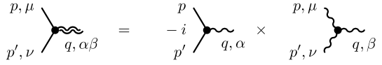
Figure 2: Factorization of the gravitino three vertex.

For the propagator of gravitons we can choose the same as in Bern:1999ji .

$$P_{hh\;\mu\alpha,\nu\beta}(p)=\frac{i\eta_{\mu\nu}\eta_{\alpha\beta}}{p^{2}+i\epsilon}\,.$$ (20)

Armed with a candidate for the gravitino three point vertex and a graviton propagator we can proceed to pursue what the four point contact interaction is. To find this we start with the four point amplitude generated by the KLT relation. From this amplitude we subtract all contributions involving the three vertex. What we are left with will form the four point contact vertex contribution. The procedure is illustrated below (see fig. 3).

Figure 3: The scheme for obtaining the four vertex through the KLT relations.

We begin by writing out the amplitude $\mathcal{M}_{4}(1^{-}_{\widetilde{h}},2^{-}_{\widetilde{h}},3^{+}_{\widetilde{h}},4^{+}_{\widetilde{h}})$. Using KLT we have

$$\begin{split}\mathcal{M}_{4}(1^{-}_{\widetilde{h}},2^{-}_{\widetilde{h}},3^{+}_{\widetilde{h}},4^{+}_{\widetilde{h}})&=-i\,s_{13}\,{\cal A}_{4}(1^{-}_{g},3^{+}_{g},2^{-}_{g},4^{+}_{g})\,{\cal A}_{4}(1^{-}_{\widetilde{g}},3^{+}_{\widetilde{g}},4^{+}_{\widetilde{g}},2^{-}_{\widetilde{g}})\,.\end{split}$$ (21)

In the above expression we can investigate the pole structure of the gluino part of the expression using the Feynman rules. We only have one diagram because the gluino-gluino-gluon vertex is helicity conserving. Thus we have (we have for convenience suppressed the notion of the reference spinors in the polarization tensors and momenta in the vertex factors as well as in the propagators.)

$$\begin{split}s_{13}\,{\cal A}_{4}(1^{-}_{\widetilde{g}},3^{+}_{\widetilde{g}},4^{+}_{\widetilde{g}},2^{-}_{\widetilde{g}})&=s_{13}\Big{(}\;\bar{\varepsilon}_{\widetilde{g}}^{-}(p_{1})\,V^{\alpha}_{\widetilde{g}g\widetilde{g}}\,\varepsilon^{+}_{\widetilde{g}}(p_{3})\;P_{gg\;\alpha\beta}\;\bar{\varepsilon}_{\widetilde{g}}^{-}(p_{2})\,V^{\beta}_{\widetilde{g}g\widetilde{g}}\,\varepsilon^{+}_{\widetilde{g}}(p_{4})\Big{)}\\ &=s_{13}\Big{(}\langle 1^{-}|\gamma_{\alpha}|3^{-}\rangle\;\frac{i}{2s_{13}}\;\langle 2^{-}|\gamma^{\alpha}|4^{-}\rangle\Big{)}\,.\end{split}$$ (22)

One sees that the prefactor of $s_{13}$ from the KLT relations cancels completely in this contribution.

Now let us now focus our attention to the gluon part. We will let the Lorentz index of particle $i$ be $\sigma_{i}$. There are three contributions corresponding to three distinct Feynman graphs.

$$\begin{split}\mathcal{A}_{4}(1^{-}_{g},3^{+}_{g},2^{-}_{g},4^{+}_{g})&\;=\;\varepsilon_{g\sigma_{1}}^{-}(p_{1})\,\varepsilon_{g\sigma_{2}}^{-}(p_{2})\,\varepsilon_{g\sigma_{3}}^{+}(p_{3})\,\varepsilon_{g\sigma_{4}}^{+}(p_{4})\,\times\\ &\hskip 14.22636pt\Big{(}V^{\sigma_{1},\sigma_{3},\mu}_{ggg}\,\Big{(}\frac{-i\eta_{\mu\nu}}{s_{13}}\Big{)}\,V^{\nu,\sigma_{2},\sigma_{4}}_{ggg}+V^{\sigma_{4},\sigma_{1},\mu}_{ggg}\,\Big{(}\frac{-i\eta_{\mu\nu}}{s_{14}}\Big{)}\,V^{\sigma_{3},\sigma_{2},\nu}_{ggg}+V^{\sigma_{1},\sigma_{3},\sigma_{2},\sigma_{4}}_{gggg}\Big{)}\,.\end{split}$$ (23)

Writing out $\mathcal{M}_{4}(1^{-}_{\widetilde{h}},2^{-}_{\widetilde{h}},3^{+}_{\widetilde{h}},4^{+}_{\widetilde{h}})$ using the above results we have

$$\begin{split}\mathcal{M}_{4}(1^{-}_{\widetilde{h}},2^{-}_{\widetilde{h}},3^{+}_{\widetilde{h}},4^{+}_{\widetilde{h}})&=-i\Big{(}\langle 1^{-}|\gamma_{\alpha}|3^{-}\rangle\,\langle 2^{-}|\gamma^{\alpha}|4^{-}\rangle\,V^{\sigma_{1},\sigma_{3},\mu}_{ggg}\Big{(}\frac{-i\eta_{\mu\nu}}{2s_{13}}\Big{)}\,V^{\nu,\sigma_{2},\sigma_{4}}_{ggg}\\ &\!\!\hskip 25.6073pt+\langle 1^{-}|\gamma_{\alpha}|3^{-}\rangle\,\langle 2^{-}|\gamma^{\alpha}|4^{-}\rangle\,V^{\sigma_{4},\sigma_{1},\mu}_{ggg}\,\Big{(}\frac{-i\eta_{\mu\nu}}{2s_{14}}\Big{)}\,V^{\sigma_{3},\sigma_{2},\nu}_{ggg}\\ &\!\!\hskip 25.6073pt+\langle 1^{-}|\gamma_{\alpha}|3^{-}\rangle\,\langle 2^{-}|\gamma^{\alpha}|4^{-}\rangle\,{1\over 2}V^{\sigma_{1},\sigma_{3},\sigma_{2},\sigma_{4}}_{gggg}\Big{)}\,\varepsilon_{g\sigma_{1}}^{-}(p_{1})\,\varepsilon_{g\sigma_{2}}^{-}(p_{2})\,\varepsilon_{g\sigma_{3}}^{+}(p_{3})\,\varepsilon_{g\sigma_{4}}^{+}(p_{4})\,.\end{split}$$ (24)

The first term gives exactly a factorized gravitino vertex structure as suggested by eq. (19) i.e.

$$\begin{split}\langle 1^{-}|\gamma_{\alpha}|3^{-}\rangle\,\langle 2^{-}|\gamma^{\alpha}|4^{-}\rangle\,V^{\sigma_{1},\sigma_{3},\mu}_{ggg}\Big{(}\frac{-i\,\eta_{\mu\nu}}{s_{13}}\Big{)}\,V^{\nu,\sigma_{2},\sigma_{4}}_{ggg}&\\ &=\Big{(}i\,\langle 1^{-}|\gamma^{\alpha}|3^{-}\rangle\,V^{\sigma_{1},\sigma_{3},\mu}_{ggg}\Big{)}\,\Big{(}\frac{i\,\eta_{\mu\nu}\eta_{\alpha\beta}}{s_{13}}\Big{)}\,\Big{(}i\langle 2^{-}|\gamma^{\beta}|4^{-}\rangle\,V^{\nu,\sigma_{2},\sigma_{4}}_{ggg}\Big{)}\,,\end{split}$$ (25)

but the second term does not appear to do that. This can however be mended by applying the Fierz rearrangement (7),

$$\langle p_{A}^{+}|\gamma_{\mu}|p_{B}^{+}\rangle\langle p_{C}^{+}|\gamma^{\mu}|p_{D}^{+}\rangle=2[AC]\langle DB\rangle=-\langle p_{A}^{+}|\gamma_{\mu}|p_{D}^{+}\rangle\langle p_{C}^{+}|\gamma^{\mu}|p_{B}^{+}\rangle\,.$$ (26)

Using this we can rearrange the gravitino amplitude so that it becomes:

$$\begin{split}\mathcal{M}_{4}(1^{-}_{\widetilde{h}},2^{-}_{\widetilde{h}},3^{+}_{\widetilde{h}},4^{+}_{\widetilde{h}})&=\varepsilon_{g\sigma_{1}}^{-}(p_{1})\,\varepsilon_{g\sigma_{2}}^{-}(p_{2})\,\varepsilon_{g\sigma_{3}}^{+}(p_{3})\,\varepsilon_{g\sigma_{4}}^{+}(p_{4})\,\times\\ &\hskip 8.5359pt\Big{(}\big{(}i\,\langle 1^{-}|\gamma^{\alpha}|3^{-}\rangle\,V^{\sigma_{1},\sigma_{3},\mu}_{ggg}\big{)}\,\frac{i\,\eta_{\alpha\beta}\eta_{\mu\nu}}{2s_{13}}\,\big{(}i\,\langle 2^{-}|\gamma^{\beta}|4^{-}\rangle\,V^{\nu,\sigma_{2},\sigma_{4}}_{ggg}\big{)}\\ &-\big{(}i\,\langle 1^{-}|\gamma^{\alpha}|4^{-}\rangle\,V^{\sigma_{4},\sigma_{1},\mu}_{ggg}\big{)}\,\frac{i\,\eta_{\alpha\beta}\eta_{\mu\nu}}{2s_{14}}\,\big{(}i\,\langle 2^{-}|\gamma^{\beta}|3^{-}\rangle\,V^{\sigma_{3},\sigma_{2},\nu}_{ggg}\big{)}\\ &+\frac{i}{4}\left(\langle 1^{-}|\gamma_{\mu}|4^{-}\rangle\,\langle 2^{-}|\gamma^{\mu}|3^{-}\rangle\,-\langle 1^{-}|\gamma_{\mu}|3^{-}\rangle\,\langle 2^{-}|\gamma^{\mu}|4^{-}\rangle\right)\,V^{\sigma_{1},\sigma_{3},\sigma_{2},\sigma_{4}}_{gggg}\Big{)}\,.\end{split}$$ (27)

By subtracting from the amplitude the parts with the gravitino three point vertex (19) and the propagator (20) according to our substraction scheme (see fig. 3) we have now recovered the structure of the gravitino contact term. It should be kept in mind that there is no $s_{12}$ channel diagram because the gravitino-gravitino-graviton vertex is helicity conserving.

Figure 4: The factorization of the gravitino contact term.

The contact term is shown diagrammatically in fig. 4. In the figure the helicities are specified. We can rewrite the contact term without reference to the helicities as follows (using eq. 7)

$$\begin{split}\left(\langle 1^{-}|\gamma_{\mu}|4^{-}\rangle\,\langle 2^{-}|\gamma^{\mu}|3^{-}\rangle-\langle 1^{-}|\gamma_{\mu}|3^{-}\rangle\,\langle 2^{-}|\gamma^{\mu}|4^{-}\rangle\right)\,V^{\sigma_{1},\sigma_{3},\sigma_{2},\sigma_{4}}_{gggg}&=\\ &\langle 1^{-}|\gamma_{\mu}|4^{-}\rangle\,\langle 2^{-}|\gamma^{\mu}|3^{-}\rangle\,\frac{i}{2}(2\eta^{\sigma_{1}\sigma_{2}}\eta^{\sigma_{3}\sigma_{4}}-\eta^{\sigma_{1}\sigma_{3}}\eta^{\sigma_{2}\sigma_{4}}-\eta^{\sigma_{1}\sigma_{4}}\eta^{\sigma_{3}\sigma_{2}})\\ &-\langle 1^{-}|\gamma_{\mu}|3^{-}\rangle\,\langle 2^{-}|\gamma^{\mu}|4^{-}\rangle\,\frac{i}{2}(2\eta^{\sigma_{1}\sigma_{2}}\eta^{\sigma_{3}\sigma_{4}}-\eta^{\sigma_{1}\sigma_{3}}\eta^{\sigma_{2}\sigma_{4}}-\eta^{\sigma_{1}\sigma_{4}}\eta^{\sigma_{3}\sigma_{2}})\\ &=\langle 1^{-}|\gamma_{\mu}|4^{-}\rangle\,\langle 2^{-}|\gamma^{\mu}|3^{-}\rangle\,\frac{i}{2}(2\eta^{\sigma_{1}\sigma_{2}}\eta^{\sigma_{3}\sigma_{4}}-2\eta^{\sigma_{1}\sigma_{3}}\eta^{\sigma_{2}\sigma_{4}})\\ &-\langle 1^{-}|\gamma_{\mu}|3^{-}\rangle\,\langle 2^{-}|\gamma^{\mu}|4^{-}\rangle\,\frac{i}{2}(2\eta^{\sigma_{1}\sigma_{2}}\eta^{\sigma_{3}\sigma_{4}}-2\eta^{\sigma_{1}\sigma_{4}}\eta^{\sigma_{3}\sigma_{2}})\,.\end{split}$$ (28)

Thus the contact term can be written (again we have here suppressed factors of $\kappa/2$)

$$\begin{split}V^{\mu,\nu,\rho,\sigma}_{abcd}&=\frac{i}{4}\Big{(}\!\gamma^{\chi}_{ab}\gamma_{\chi\,cd}(\eta^{\mu\rho}\eta^{\nu\sigma}\!-\eta^{\mu\sigma}\eta^{\nu\rho})+\gamma^{\chi}_{ac}\gamma_{\chi\,bd}(\eta^{\mu\sigma}\eta^{\nu\rho}\!-\eta^{\mu\nu}\eta^{\rho\sigma})+\gamma^{\chi}_{ad}\gamma_{\chi\,bc}(\eta^{\mu\nu}\eta^{\rho\sigma}\!-\eta^{\mu\rho}\eta^{\nu\sigma})\!\Big{)}\,.\end{split}$$ (29)

To leading order in $\bar{\Psi}$, $\Psi$ and $h$ one can thus instead of (13) use the following interaction Lagrangian:

$$\begin{split}\mathcal{L}&=\frac{i\kappa}{4}\Big{(}\bar{\Psi}_{\mu}\gamma^{\nu}(\partial^{\rho}\Psi^{\mu})h_{\rho\nu}-\bar{\Psi}_{\mu}\gamma^{\nu}(\partial^{\mu}\Psi^{\rho})h_{\rho\nu}-\bar{\Psi}^{\rho}\gamma^{\nu}\Psi^{\mu}(\partial_{\mu}h_{\rho\nu})\Big{)}+\frac{\kappa^{2}}{64}\bar{\Psi}_{\mu}\gamma_{\nu}\Psi_{\rho}\bar{\Psi}^{\mu}\gamma^{\nu}\Psi^{\rho}\,.\end{split}$$ (30)

III.2 Analysis of two gravitino two graviton amplitude

Let us now turn to the amplitude of two gravitinos and two gravitons

$$\begin{split}\mathcal{M}_{4}(1^{-}_{\widetilde{h}},2^{-}_{h},3^{+}_{\widetilde{h}},4^{+}_{h})&=-i\,s_{14}\,{\cal A}_{4}(1^{-}_{\widetilde{g}},4^{+}_{g},2^{-}_{g},3^{+}_{\widetilde{g}})\,{\cal A}_{4}(1^{-}_{g},2^{-}_{g},3^{+}_{g},4^{+}_{g})\,.\end{split}$$ (31)

There are four diagrams to be considered. They are shown below in fig. 5.

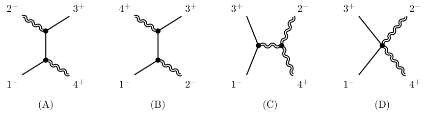
Figure 5: The four diagrams we need to compute the amplitude $\mathcal{M}_{4}(1^{-}_{\widetilde{h}},2^{-}_{h},3^{+}_{\widetilde{h}},4^{+}_{h})$.

To calculate the diagrams (A) and (B), we need in addition to the three vertex with one graviton leg (see (19)) a propagator for the gravitino. Inspired by (20) and the propagator used in Das:1976ct we choose

$$\begin{split}P_{\widetilde{h}\widetilde{h}\;\mu\nu}(p)&=\frac{-i\,\cancel{p}\eta_{\mu\nu}}{p^{2}+i\epsilon}\,.\end{split}$$ (32)

This propagator is shown diagrammatically in fig. 6.

Figure 6: The gravitino propagator.

In order to compute diagram (C) we need a graviton three vertex in addition to the already discussed Feynman rules. Here we choose (we have here suppressed factors of $\kappa/2$)

$$\begin{split}V^{\mu\nu,\alpha\beta,\rho\sigma}_{hhh}(p,q,p^{\prime})&=-i\;V^{\mu,\alpha,\rho}_{ggg}(p,q,p^{\prime})\,V^{\nu,\beta,\sigma}_{ggg}(p,q,p^{\prime})\\ &=-i\left(\frac{i}{\sqrt{2}}\right)^{2}\Big{(}(p-q)^{\rho}\,\eta^{\mu\alpha}+(q-p^{\prime})^{\mu}\,\eta^{\alpha\rho}+(p^{\prime}-p)^{\alpha}\,\eta^{\rho\mu}\Big{)}\\ &\hskip 59.46614pt\times\Big{(}(p-q)^{\sigma}\,\eta^{\beta\nu}+(q-p^{\prime})^{\nu}\,\eta^{\sigma\beta}+(p^{\prime}-p)^{\beta}\,\eta^{\nu\sigma}\Big{)}\,.\end{split}$$ (33)

which is shown diagrammatically in fig. 7:

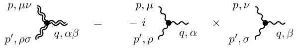
Figure 7: The graviton three vertex.

It is convenient to split the diagrams $(A)$, $(B)$, $(C)$ and $(D)$ into a purely gluonic diagram and a mixed gluon/gluino diagram and let the poles be associated with the purely gluonic diagram (we will define $\tilde{\Pi}\equiv\varepsilon_{g\,\sigma_{1}}^{-}(p_{1})\,\varepsilon_{g\,\sigma_{2}}^{-}(p_{2})\,\varepsilon_{g\,\sigma_{3}}^{+}(p_{3})\,\varepsilon_{g\,\sigma_{4}}^{+}(p_{4})$ and $\Pi\equiv\varepsilon_{g\,\rho_{2}}^{-}(p_{2})\,\varepsilon_{g\,\rho_{4}}^{+}(p_{4})$ and we have suppressed the notion of the momenta in the vertex factors as well as in the propagators for convenience):

$$\begin{split}(A)&=\tilde{\Pi}\,\Pi\,\langle 1^{-}|V_{\widetilde{h}\widetilde{h}h}^{\sigma_{1},\kappa,\rho_{4}\sigma_{4}}\,P_{\widetilde{h}\widetilde{h}\;\kappa\lambda}\,V_{\widetilde{h}h\widetilde{h}}^{\lambda,\rho_{2}\sigma_{2},\sigma_{3}}|3^{-}\rangle\\ &=i\;\tilde{\Pi}\,\Pi\,\langle 1^{-}|\big{(}V_{\widetilde{g}\widetilde{g}g}^{\rho_{4}}\,V_{ggg}^{\sigma_{1},\kappa,\sigma_{4}}\big{)}\,\big{(}s_{14}P_{\widetilde{g}\widetilde{g}}\,P_{gg\;\kappa\lambda}\big{)}\,\big{(}V_{\widetilde{g}g\widetilde{g}}^{\rho_{2}}\,V_{ggg}^{\lambda,\sigma_{2},\sigma_{3}}\big{)}|3^{-}\rangle\\ &=i\;\tilde{\Pi}\,\Pi\,\big{(}\langle 1^{-}|V_{\widetilde{g}g\widetilde{g}}^{\rho_{4}}\,s_{14}\,P_{\widetilde{g}\widetilde{g}}\,V_{\widetilde{g}g\widetilde{g}}^{\rho_{2}}|3^{-}\rangle\big{)}\,\big{(}V_{ggg}^{\sigma_{1},\kappa,\sigma_{4}}\,P_{gg;\kappa\lambda}\,V_{ggg}^{\lambda,\sigma_{2},\sigma_{3}}\big{)}\,.\end{split}$$ (34)

$$\begin{split}(B)&=\tilde{\Pi}\,\Pi\,\langle 1^{-}|V_{\widetilde{h}h\widetilde{h}}^{\sigma_{1},\rho_{2}\sigma_{2},\kappa}\,P_{\widetilde{h}\widetilde{h}\;\kappa\lambda}\,V_{\widetilde{h}\widetilde{h}h}^{\lambda,\sigma_{3},\rho_{4}\sigma_{4}}|3^{-}\rangle\\ &=i\;\tilde{\Pi}\,\Pi\,\langle 1^{-}|\big{(}V_{\widetilde{g}g\widetilde{g}}^{\rho_{2}}\,V_{ggg}^{\sigma_{1},\sigma_{2},\kappa}\big{)}\,\big{(}s_{12}\,P_{\widetilde{g}\widetilde{g}}\,P_{gg\;\kappa\lambda}\big{)}\,\big{(}V_{\widetilde{g}\widetilde{g}g}^{\rho_{4}}\,V_{ggg}^{\lambda,\sigma_{3},\sigma_{4}}\big{)}|3^{-}\rangle\\ &=i\;\tilde{\Pi}\,\Pi\,\big{(}\langle 1^{-}|V_{\widetilde{g}g\widetilde{g}}^{\rho_{2}}\,s_{12}\,P_{\widetilde{g}\widetilde{g}}\,V_{\widetilde{g}\widetilde{g}g}^{\rho_{4}}|3^{-}\rangle\big{)}\big{(}V_{ggg}^{\sigma_{1},\sigma_{2},\kappa}\,P_{gg\;\kappa\lambda}\,V_{ggg}^{\lambda,\sigma_{3},\sigma_{4}}\big{)}\,.\end{split}$$ (35)

$$\begin{split}(C)&=\tilde{\Pi}\,\Pi\,\langle 1^{-}|V_{\widetilde{h}h\widetilde{h}}^{\sigma_{1},\kappa\lambda,\sigma_{3}}|3^{-}\rangle\,P_{hh\kappa\lambda,\alpha\beta}\,V_{hhh}^{\alpha\beta,\rho_{2}\sigma_{2},\rho_{4}\sigma_{4}}\varepsilon_{\sigma_{1}}^{-}(p_{1})\\ &=i\;\tilde{\Pi}\,\Pi\,\langle 1^{-}|\big{(}V_{\widetilde{g}g\widetilde{g}}^{\kappa}\,V_{ggg}^{\sigma_{1},\lambda,\sigma_{3}}\big{)}|3^{-}\rangle\,\big{(}s_{13}\,P_{gg\lambda,\beta}\,P_{gg\;\kappa\alpha}\big{)}\,\big{(}V_{ggg}^{\alpha,\rho_{2},\rho_{4}}\,V_{ggg}^{\beta,\sigma_{2},\sigma_{4}}\big{)}\\ &=i\;\tilde{\Pi}\,\Pi\,\big{(}\langle 1^{-}|V_{\widetilde{g}g\widetilde{g}}^{\kappa}|3^{-}\rangle\,s_{13}\,P_{gg\;\kappa\alpha}\,V_{ggg}^{\alpha,\rho_{2},\rho_{4}}\big{)}\,\big{(}V_{ggg}^{\sigma_{1},\lambda,\sigma_{3}}\,P_{gg\lambda,\beta}\,V_{ggg}^{\beta,\sigma_{2},\sigma_{4}}\big{)}\,.\end{split}$$ (36)

We will focus on the gluino parts of these expressions. We get (see fig. 8).

Figure 8: The three different gluon/gluino diagrams with cancelled poles.

Using this we can write $(A)$, $(B)$ and $(C)$ as

$$\begin{split}(A)&=iX\,\tilde{\Pi}\,\big{(}V_{ggg}^{\sigma_{1},\kappa,\sigma_{4}}\,P_{gg\;\kappa\lambda}\,V_{ggg}^{\lambda,\sigma_{2},\sigma_{3}}\big{)}\,,\\ (B)&=i\,(X-Y)\,\tilde{\Pi}\,\big{(}V_{ggg}^{\sigma_{1},\sigma_{2},\kappa}\,P_{gg\;\kappa\lambda}\,V_{ggg}^{\lambda,\sigma_{3},\sigma_{4}}\big{)}\,,\\ (C)&=i\,Y\,\tilde{\Pi}\,\big{(}V_{ggg}^{\sigma_{1},\lambda,\sigma_{3}}\,P_{gg\;\lambda\beta}\,V_{ggg}^{\beta,\sigma_{2},\sigma_{4}}\big{)}\,.\end{split}$$ (37)

Let us now sum the contributions from the three diagrams:

$$\begin{split}(A)+(B)+(C)&=i\,X\,\tilde{\Pi}\,\big{(}V_{ggg}^{\sigma_{1},\kappa,\sigma_{4}}\,P_{gg\;\kappa\lambda}\,V_{ggg}^{\lambda,\sigma_{2},\sigma_{3}}+V_{ggg}^{\sigma_{1},\sigma_{2},\kappa}\,P_{gg;\kappa\lambda}\,V_{ggg}^{\lambda,\sigma_{3},\sigma_{4}}\big{)}\\ &+i\,Y\,\tilde{\Pi}\,\big{(}V_{ggg}^{\sigma_{1},\lambda,\sigma_{3}}\,P_{gg\;\lambda\beta}\,V_{ggg}^{\beta,\sigma_{2},\sigma_{4}}-V_{ggg}^{\sigma_{1},\sigma_{2},\kappa}\,P_{gg\;\kappa\lambda}\,V_{ggg}^{\lambda,\sigma_{3},\sigma_{4}}\big{)}\,.\end{split}$$ (38)

By inspecting the terms in the parentheses, we notice that each of them consists of the pole diagrams from color-ordered gluon amplitudes. Hence if we add the gluon contact term $V^{\sigma_{1},\sigma_{2},\sigma_{3},\sigma_{4}}_{gggg}$ and $V^{\sigma_{1},\sigma_{2},\sigma_{4},\sigma_{3}}_{gggg}$ by hand we arrive at

$$\begin{split}(A)+(B)+(C)&=i\,X\,\mathcal{A}(1_{g},2_{g},3_{g},4_{g})-i\,X\,\tilde{\Pi}\,V^{\sigma_{1},\sigma_{2},\sigma_{3},\sigma_{4}}_{gggg}\\ &+i\,Y\,\mathcal{A}(1_{g},2_{g},4_{g},3_{g})-i\,Y\,\tilde{\Pi}\,V^{\sigma_{1},\sigma_{2},\sigma_{4},\sigma_{3}}_{gggg}\,.\end{split}$$ (39)

If we rewrite $X$ and $Y$ in terms of the gluino/gluon diagrams we have

$$\begin{split}(A)+(B)+(C)&=i\,s_{14}\,\big{(}\langle 1^{-}|V_{\widetilde{g}g\widetilde{g}}^{\rho_{4}}\,P_{\widetilde{g}\widetilde{g}}\,V_{\widetilde{g}g\widetilde{g}}^{\rho_{2}}|3^{-}\rangle\big{)}\,\Pi\,\mathcal{A}(1_{g},2_{g},3_{g},4_{g})\\ &+i\,s_{13}\,\big{(}\langle 1^{-}|V_{\widetilde{g}g\widetilde{g}}^{\kappa}|3^{-}\rangle\,P_{gg\;\kappa\alpha}\,V_{ggg}^{\alpha,\rho_{2},\rho_{4}}\big{)}\,\Pi\,\mathcal{A}(1_{g},2_{g},4_{g},3_{g})\\ &-i\,X\,\tilde{\Pi}\,V^{\sigma_{1},\sigma_{2},\sigma_{3},\sigma_{4}}_{gggg}-i\,Y\,\tilde{\Pi}\,V^{\sigma_{1},\sigma_{2},\sigma_{4},\sigma_{3}}_{gggg}\,.\end{split}$$ (40)

We can now use that $s_{13}\,\mathcal{A}(1_{g},2_{g},4_{g},3_{g})=s_{14}\,\mathcal{A}(1_{g},2_{g},3_{g},4_{g})$ to rewrite

$$\begin{split}(A)+(B)+(C)&=i\,s_{14}\,\mathcal{A}(1_{\widetilde{g}},3_{\widetilde{g}},2_{g},4_{g})\,\mathcal{A}(1_{g},2_{g},3_{g},4_{g})-i\,X\,\tilde{\Pi}\,V^{\sigma_{1},\sigma_{2},\sigma_{3},\sigma_{4}}_{gggg}-i\,Y\,\tilde{\Pi}\,V^{\sigma_{1},\sigma_{2},\sigma_{4},\sigma_{3}}_{gggg}\\ &=-i\,s_{14}\,\mathcal{A}(1_{\widetilde{g}},4_{g},2_{g},3_{\widetilde{g}})\,\mathcal{A}(1_{g},2_{g},3_{g},4_{g})-i\,X\,\tilde{\Pi}\,V^{\sigma_{1},\sigma_{2},\sigma_{3},\sigma_{4}}_{gggg}-i\,Y\,\tilde{\Pi}\,V^{\sigma_{1},\sigma_{2},\sigma_{4},\sigma_{3}}_{gggg}\,.\end{split}$$ (41)

Thus we can read off the gravitino contact term as $i\,X\,\tilde{\Pi}\,V^{\sigma_{1},\sigma_{2},\sigma_{3},\sigma_{4}}_{gggg}+i\,Y\,\tilde{\Pi}\,V^{\sigma_{1},\sigma_{2},\sigma_{4},\sigma_{3}}_{gggg}$. That correspond to the graviton/gravitino vertex rule (we have again suppressed all factors of $\kappa/2$ for convenience).

$$\begin{split}V^{\mu,\nu,\alpha\beta,\kappa\lambda}_{\widetilde{h}\widetilde{h}hh}(p,p^{\prime},q,\widetilde{q})&=\frac{i}{8}\,\bigg{[}3\left(\eta^{\mu\beta}\eta^{\nu\lambda}-\eta^{\mu\lambda}\eta^{\nu\beta}\right)\Big{(}(\cancel{q}-\cancel{\widetilde{q}})\eta^{\alpha\kappa}+\gamma^{\alpha}(p+p^{\prime}-q)^{\kappa}+\gamma^{\kappa}(\widetilde{q}-p-p^{\prime})^{\alpha}\Big{)}\\ &\hskip 14.22636pt-\big{(}\gamma^{\kappa}(\cancel{\widetilde{q}}+\cancel{p})\gamma^{\alpha}+\gamma^{\alpha}(\cancel{p}+\cancel{q})\gamma^{\kappa}\big{)}\big{(}2\eta^{\mu\nu}\eta^{\beta\lambda}-\eta^{\mu\beta}\eta^{\nu\lambda}-\eta^{\mu\lambda}\eta^{\nu\beta}\big{)}\bigg{]}\,.\end{split}$$ (42)

At the level of the Lagrangian this correspond to

$$\begin{split}\mathcal{L}&=\frac{3i\kappa^{2}}{64}\bar{\Psi}_{\mu}\gamma^{\nu}\Psi_{\rho}(\partial^{\chi}h^{\rho\sigma})h^{\mu\tau}\big{(}2\eta_{\chi\tau}\eta_{\nu\sigma}-\eta_{\nu\tau}\eta_{\chi\sigma}-\eta_{\sigma\tau}\eta_{\nu\chi}\big{)}\\ &+\frac{i\kappa^{2}}{128}\bar{\Psi}_{\alpha}\gamma^{\nu}h_{\beta\nu}\cancel{\partial}(h_{\gamma\mu}\gamma^{\mu}\Psi_{\delta})\times\big{(}2\eta^{\alpha\delta}\eta^{\beta\gamma}-\eta^{\alpha\beta}\eta^{\gamma\delta}-\eta^{\alpha\gamma}\eta^{\beta\delta}\big{)}\,.\end{split}$$ (43)

The vertex is shown diagrammatically below (see fig. 9).

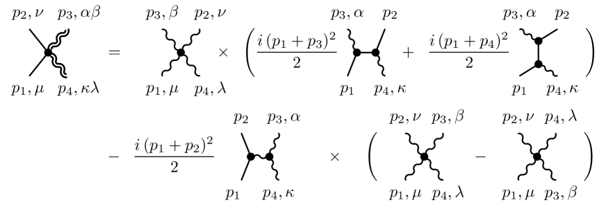
Figure 9: The factorization of the gravitino-graviton contact term.

III.2.1 Analysis of five points, four gravitino one graviton amplitude

Finally, as a check of the Feynman vertex rules of the previous section we turn to the amplitude of four gravitinos and one graviton. There are five different Feynman graph topologies as shown below (see fig. 10).

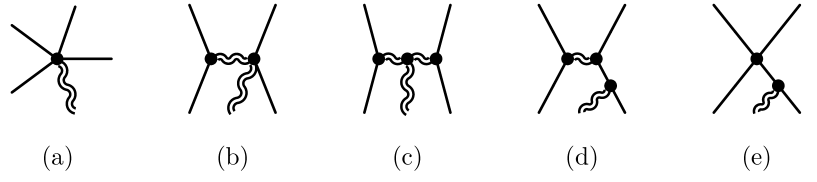
Figure 10: The five different diagram topologies for the five point function

The diagrams of topology (b), (c), (d) and (e) can be created from the Feynman rules found in the four point case. Contribution (a) requires the five point contact interaction. By a careful analysis of all contributions it turns out that no such term is necessary to get to the full amplitude. Thus the four gravitino one graviton contact vertex factor (a) is vanishing.

The vanishing of the five point interaction can also be understood from the perspective of the Lagrangian given the manifest left / right mover separated structure of such a interaction term and the odd number of Lorentz indices which subsequently have to be contracted with each other. However, it is interesting that the KLT inspired formalism yields this result with such ease. Similar arguments appear to hold for interaction terms in the Lagrangian which have four gravitinos and any odd number of gravitons.

IV Conclusion

In this paper we have extended the analysis of Bern and Grant Bern:1999ji to gravitino scattering. Using Yang-Mills theory and the KLT relations as the only input we have derived complete Feynman rules for gravitino scattering verified until five-point scattering with one external graviton. The Feynman rules derived via KLT have the useful property that they are simpler than results derived from a conventional analysis and they are manifestly factorized into a gluon and a gluino part. It seems clear that the organizational principles induced by KLT rearranges the Lagrangian in useful and simpler ways than traditional gauge choices.

Using a KLT inspired left-right separation of fields as a way to organize and symmetrize vertex interactions is not limited to graviton and gravitino interactions. As a task for future research it would be very interesting to further investigate how KLT possibly could be used to simplify Feynman rules and computations for many other types of matter.

References

• (1) H. Kawai, D. C. Lewellen and S. H. H. Tye, Nucl. Phys. B 269, 1 (1986).
• (2) H. Kuijf, Phys. Lett. B 211, 91 (1988); Z. Bern and D. C. Dunbar, Nucl. Phys. B 379, 562 (1992); Z. Bern, D. C. Dunbar and T. Shimada, Phys. Lett. B 312, 277 (1993) [hep-th/9307001]; D. C. Dunbar and P. S. Norridge, Nucl. Phys. B 433, 181 (1995) [hep-th/9408014]; D. C. Dunbar and P. S. Norridge, Class. Quant. Grav. 14 (1997) 351 [hep-th/9512084]; D. C. Dunbar and N. W. P. Turner, Class. Quant. Grav. 20, 2293 (2003) [hep-th/0212160]; D. C. Dunbar, B. Julia, D. Seminara and M. Trigiante, JHEP 0001, 046 (2000) [hep-th/9911158].
• (3) Z. Bern, L. J. Dixon, D. C. Dunbar, M. Perelstein and J. S. Rozowsky, Nucl. Phys. B 530, 401 (1998) [hep-th/9802162]; Z. Bern, L. J. Dixon, M. Perelstein and J. S. Rozowsky, Phys. Lett. B 444, 273 (1998) [hep-th/9809160]; Z. Bern, L. J. Dixon, M. Perelstein and J. S. Rozowsky, Nucl. Phys. B 546, 423 (1999) [hep-th/9811140]; Z. Bern, L. J. Dixon, M. Perelstein, D. C. Dunbar and J. S. Rozowsky, Class. Quant. Grav. 17, 979 (2000) [hep-th/9911194].
• (4) Z. Bern and A. K. Grant, Phys. Lett. B 457, 23 (1999) [hep-th/9904026].
• (5) E. Witten, Commun. Math. Phys. 252, 189 (2004) [hep-th/0312171].
• (6) F. Cachazo and P. Svrcek, PoS RTN2005, 004 (2005) [hep-th/0504194].
• (7) Z. Bern, L. J. Dixon and D. A. Kosower, Annals Phys. 322, 1587 (2007) [0704.2798 [hep-ph]].
• (8) S. Giombi, R. Ricci, D. Robles-Llana and D. Trancanelli, JHEP 0407, 059 (2004) [hep-th/0405086].
• (9) Z. Bern, N. E. J. Bjerrum-Bohr and D. C. Dunbar, JHEP 0505, 056 (2005) [hep-th/0501137].
• (10) J. Bedford, A. Brandhuber, B. Spence and G. Travaglini, Nucl. Phys. B 721, 98 (2005) [hep-th/0502146]; F. Cachazo and P. Svrček, hep-th/0502160.
• (11) N. E. J. Bjerrum-Bohr, D. C. Dunbar and H. Ita, Phys. Lett. B 621, 183 (2005) [hep-th/0503102]; hep-th/0606268; hep-th/0608007.
• (12) N. E. J. Bjerrum-Bohr, D. C. Dunbar, H. Ita, W. B. Perkins and K. Risager, JHEP 0601, 009 (2006) [hep-th/0509016].
• (13) N. E. J. Bjerrum-Bohr, D. C. Dunbar, H. Ita, W. B. Perkins and K. Risager, JHEP 0612, 072 (2006) [hep-th/0610043].
• (14) P. Benincasa, C. Boucher-Veronneau and F. Cachazo, JHEP 0711, 057 (2007) [hep-th/0702032].
• (15) Z. Bern, J. J. Carrasco, D. Forde, H. Ita and H. Johansson, Phys. Rev. D 77, 025010 (2008) [0707.1035 [hep-th]].
• (16) S. Ananth and S. Theisen, Phys. Lett. B 652, 128 (2007) [0706.1778 [hep-th]]; S. Ananth, Phys. Lett. B 664, 219 (2008) [0803.1494 [hep-th]]; S. Ananth, Fortsch. Phys. 57, 857 (2009) [0902.3128 [hep-th]].
• (17) H. Elvang and D. Z. Freedman, JHEP 0805, 096 (2008) [0710.1270 [hep-th]]; M. Bianchi, H. Elvang and D. Z. Freedman, JHEP 0809, 063 (2008) [0805.0757 [hep-th]]; H. Elvang, D. Z. Freedman and M. Kiermaier, 0911.3169 [hep-th].
• (18) A. Hall, Phys. Rev. D 77, 124004 (2008) [0803.0215 [hep-th]].
• (19) N. E. J. Bjerrum-Bohr and P. Vanhove, JHEP 0804, 065 (2008) [0802.0868 [hep-th]]; Fortsch. Phys. 56, 824 (2008) [0806.1726 [hep-th]].
• (20) N. Arkani-Hamed and J. Kaplan, JHEP 0804, 076 (2008) [0801.2385 [hep-th]].
• (21) N. E. J. Bjerrum-Bohr and P. Vanhove, JHEP 0810, 006 (2008) [0805.3682 [hep-th]].
• (22) Z. Bern, J. J. M. Carrasco and H. Johansson, Phys. Rev. D 78, 085011 (2008) [0805.3993 [hep-ph]].
• (23) N. Arkani-Hamed, F. Cachazo and J. Kaplan, 0808.1446 [hep-th]; N. Arkani-Hamed, F. Cachazo, C. Cheung and J. Kaplan, 0903.2110 [hep-th].
• (24) S. Badger, N. E. J. Bjerrum-Bohr and P. Vanhove, JHEP 0902, 038 (2009) [0811.3405 [hep-th]].
• (25) P. Katsaroumpas, B. Spence and G. Travaglini, JHEP 0908, 096 (2009) [0906.0521 [hep-th]].
• (26) Z. Bern, L. J. Dixon and R. Roiban, Phys. Lett. B 644, 265 (2007) [hep-th/0611086]; H. Johansson, D. A. Kosower and R. Roiban, Phys. Rev. Lett. 98, 161303 (2007) [hep-th/0702112]; Z. Bern, J. J. M. Carrasco, L. J. Dixon, H. Johansson and R. Roiban, Phys. Rev. D 78, 105019 (2008) [0808.4112 [hep-th]]; Z. Bern, J. J. Carrasco, L. J. Dixon, H. Johansson and R. Roiban, Phys. Rev. Lett. 103, 081301 (2009) [0905.2326 [hep-th]].
• (27) C. Cheung and D. O’Connell, JHEP 0907, 075 (2009) [0902.0981 [hep-th]].
• (28) N. E. J. Bjerrum-Bohr, P. H. Damgaard and P. Vanhove, Phys. Rev. Lett.  103, 161602 (2009) [0907.1425 [hep-th]].
• (29) S. Stieberger, 0907.2211 [hep-th]; 0910.0180 [hep-th].
• (30) R. Boels, JHEP 1001, 010 (2010) [0908.0738 [hep-th]].
• (31) Y. X. Chen, Y. J. Du and Q. Ma, Nucl. Phys.  B 824, 314 (2010) [0901.1163 [hep-th]]; 1001.0060 [hep-th].
• (32) M. B. Green, J. G. Russo and P. Vanhove, JHEP 0702, 099 (2007) [hep-th/0610299]; M. B. Green, J. G. Russo and P. Vanhove, Phys. Rev. Lett.  98, 131602 (2007) [hep-th/0611273]; N. Berkovits, M. B. Green, J. G. Russo and P. Vanhove, JHEP 0911, 063 (2009) [0908.1923 [hep-th]].
• (33) S. Weinberg, PhysicaA 96, 327 (1979); J. F. Donoghue, Phys. Rev. D 50 (1994) 3874 [gr-qc/9405057]; N. E. J. Bjerrum-Bohr, J. F. Donoghue and B. R. Holstein, Phys. Rev. D 67, 084033 (2003) [hep-th/0211072]; Phys. Rev. D 68, 084005 (2003) [hep-th/0211071].
• (34) Z. Bern, A. De Freitas and H. L. Wong, Phys. Rev. Lett. 84, 3531 (2000) [hep-th/9912033].
• (35) N. E. J. Bjerrum-Bohr, Phys. Lett. B 560, 98 (2003) [hep-th/0302131]; Nucl. Phys. B 673, 41 (2003) [hep-th/0305062]; N. E. J. Bjerrum-Bohr and K. Risager, Phys. Rev. D 70, 086011 (2004) [hep-th/0407085].
• (36) Z. Bern, Living Rev. Rel. 5, 5 (2002) [gr-qc/0206071].
• (37) Z. Xu, D. H. Zhang and L. Chang, Nucl. Phys. B 291, 392 (1987).
• (38) W. Rarita and J. Schwinger, Phys. Rev. 60, 61 (1941).
• (39) D. Z. Freedman, P. van Nieuwenhuizen and S. Ferrara, Phys. Rev. D 13, 3214 (1976).
• (40) S. Ferrara, F. Gliozzi, J. Scherk and P. Van Nieuwenhuizen, Nucl. Phys. B 117, 333 (1976).
• (41) A. K. Das and D. Z. Freedman, Nucl. Phys. B 114, 271 (1976).
• (42) M. T. Grisaru, H. N. Pendleton and P. van Nieuwenhuizen, Phys. Rev. D 15, 996 (1977).
• (43) M. T. Grisaru and H. N. Pendleton, Nucl. Phys. B 124, 81 (1977).
• (44) N. K. Nielsen, M. T. Grisaru, H. Romer and P. van Nieuwenhuizen, Nucl. Phys. B 140, 477 (1978).
• (45) M. T. Grisaru, D. Z. Freedman and P. van Nieuwenhuizen, Phys. Lett. B 71, 377 (1977).
• (46) M. L. Mangano and S. J. Parke, Phys. Rept. 200 (1991) 301 [hep-th/0509223].
• (47) L. J. Dixon, hep-ph/9601359.