The XMM-Newton Detection of Extended Emission from the Nova Remnant of T Pyxidis

Abstract

We report the detection of an extended X-ray nebulosity with an elongation from northeast to southwest in excess of 15^′′ in a radial profile and imaging of the recurrent nova T Pyx using the archival data obtained with the X-ray Multi-Mirror Mission ($XMM$-$Newton$ ), European Photon Imaging Camera (pn instrument). The signal to noise ratio (S/N) in the extended emission (above the point source and the background) is 5.2 over the 0.3-9.0 keV energy range and 4.9 over the 0.3-1.5 keV energy range. We calculate an absorbed X-ray flux of 2.3$\times$10^-14 erg cm^-2 s^-1 with a luminosity of 6.0$\times$10³² erg s^-1 from the remnant nova in the 0.3-10.0 keV band. The source spectrum is not physically consistent with a blackbody emission model as a single model or a part of a two-component model fitted to the $XMM$-$Newton$ data ($kT{\rm{}_{BB}}$ $>$ 1 keV). The spectrum is best described by two MEKAL plasma emission models with temperatures at 0.2${}^{+0.7}_{-0.1}$ keV and 1.3${}^{+1.0}_{-0.4}$ keV. The neutral hydrogen column density derived from the fits is significantly more in the hotter X-ray component than the cooler one which we may be attributed to the elemental enhancement of nitrogen and oxygen in the cold material within the remnant. The shock speed calculated from the softer X-ray component of the spectrum is 300-800 km s^-1 and is consistent with the expansion speeds of the nova remnant derived from the $Hubble\ Space\ Telescope$ ($HST$) and ground-based optical wavelength data. Our results suggest that the detected X-ray emission may be dominated by shock-heated gas from the nova remnant.

1 Introduction

Classical novae (CNe) outbursts are the explosive ignition of accreted material on the surface of the white dwarf (WD) in a cataclysmic variable (CV) as a result of a thermonuclear runaway causing the ejection of 10^-7 to 10^-3 M_⊙ of material at velocities up to several thousand kilometers per second (Shara 1989; Livio 1994; Starrfield 2001; Bode $\&$ Evans 2008). Though there has only been one previous (and one very marginal) detection of old CNe remnants in the X-ray wavelengths (Balman & Ögelman 1999; Balman 2005,2006; Pekön & Balman 2008), CNe have been detected in the hard X-rays (above 1 keV) as a result of accretion, wind-wind and/or blast wave interaction in the outburst stage (O’Brien et al. 1994; Krautter et al. 1996; Balman, Krautter, Ögelman 1998, Mukai & Ishida 2001, Orio et al. 2001; Ness et al. 2003; Hernanz & Sala 2002,2007; Page et al. 2009). Recurrent novae (RNe) are a type of CNe where outbursts recur with intervals of several decades (Webbink et al. 1987; Hachisu $\&$ Kato 2001; Bode & Evans 2008). In general, these systems are expected to have high accretion rates of 10^-8 to 10^-7 M_⊙ yr^-1 onto massive WDs close to the Chandrasekhar limit; occurrence of recurrent outbursts in relatively less massive WDs is also possible (Starrfield, Sparks, Truran 1985; Prialnik & Kovetz 1995; Yaron et al. 2005). RNe are detected in the hard X-rays in the outburst stage as a result of wind-wind and/or blast wave interaction during the outburst stage (Orio et al. 2005; Greiner & Di Stefano 2002; Bode et al. 2006; Sokoloski et al. 2006; Drake et al. 2009; Ness et al. 2009). Recently, extended X-ray emission associated with the radio jet of the recurrent nova RS Oph is discovered (Luna et al. 2009).

Recurrent nova T Pyx has 5 recorded outbursts in 1890, 1902, 1920, 1944, and 1966 (Webbink et al. 1987). Ground-based CCD observations (Shara et al. 1989) show the existence of at least two of the shells extending to a size of $\sim$ 20^′′ in diameter and also a faint [OIII] shell has been found. $Hubble\ Space\ Telescope$ ($HST$; 1994-2007) and ground-based imaging of the shell around T Pyx show thousands of knots in H$\alpha$ and [NII] with expansion velocities of about 350-715 km s^-1, with shell expansion speed around 500 km s^-1 (Shara et al. 1997; O’Brien & Cohen 1998; Schaefer, Pagnotta & Shara 2010). The $HST$ observations support an interacting shells model producing the clumping, shock heating, and emission lines. Schaefer et al. (2010) show that most of the knots have not decelerated and are powered by the RN outbursts and originate from a CN outburst of the year 1866. T Pyx is suggested to be a wind-driven source (due to the high mass accretion rate of $\dot{M}$ $\sim$ 1$\times$ $10^{-7}$ M_⊙ yr^-1) and a Super Soft X-ray source (SSS) (Patterson et al. 1998). On the other hand, Greiner & Di Stefano (2002) reports a ROSAT non-detection of the source in December 1998 excluding the possibility of the existence of a SSS. Gilmozzi & Selvelli (2007) and Selvelli et al. (2008) show that the UV+opt+IR spectrum of T Pyx is dominated by the accretion disk and the continuum in the UV can be represented by a blackbody of T $\sim$ 34000 K with $\dot{M}$ $\sim$ 1$\times$10^-8 M_⊙ yr^-1. Their detailed study based on the UV data excludes the possibility that T Pyx is a SSS and Selvelli et al. (2008) uses this X-ray Multi-Mirror Mission ($XMM$-$Newton$ ) data set to show that a SSS nature is not supported.

2 The Data and Observation

The $XMM$-$Newton$ Observatory (Jansen et al. 2001) has three 1500 cm² X-ray telescopes each with an European Photon Imaging Camera (EPIC) at the focus; two of which have Multi-Object Spectrometer (MOS) CCDs (Turner et al. 2001) and the last one uses pn CCDs (Strüder et al. 2001) for data recording. T Pyx was observed (pointed observation) by $XMM$-$Newton$ for a duration of 51 ks between 2006 November 9 UT 19:22:59 and 2006 November 10 UT 09:02:31 with a slight off-axis angle of about 1^′. A medium optical blocking filter was used with all the EPIC cameras and the pn, MOS1 and MOS2, instruments were operated in the full frame imaging mode. We analysed the pipeline-processed data using Science Analysis Software (SAS) version 8.0.5. Data (single- and double-pixel events, i.e., patterns 0–4 with Flag=0 option) were extracted from a circular region of radius 15^′′ for pn, MOS1 and MOS2 in order to perform spectral analysis together with the background events extracted from a source free zone normalised to the source extraction area. In this paper, we will present an image obtained by the EPIC pn since it has more source photons due to its better sensitivity compared with the MOS1 and MOS2 instruments. However, we simultaneously use EPIC pn, EPIC MOS1 and EPIC MOS2 data to determine the X-ray spectrum of the source and increase the number of data points in the fitting process. We cleaned the pipeline-processed event file from the existing flaring episodes by creating user-select good time intervals (gti) with a count rate threshold $<$ 0.08 c s^-1 for the two MOS and $<$ 0.11 c s^-1 for the pn instruments over the 0.3-9.0 keV energy range. This method cleaned the flares. Within the extraction area indicated above, the final source count rates were 0.007$\pm$0.001 c s^-1 for pn, 0.003$\pm$0.001 c s^-1 for MOS1 and MOS2 with the effective exposure times of 30.6 ksec, 39.7 ksec and 38.8 ksec for the pn, MOS1 and MOS2 instruments, respectively.

3 Analysis and Results

3.1 The X-ray Image and the Radial Profile of T Pyx

The pipeline-processed and cleaned event files are used to calculate the X-ray image of T Pyx and its vicinity. The largest size of the shell of T Pyx is determined to be 10^′′ in radius (see the Introduction). Figure 1 shows an X-ray intensity image between 0.3 and 9.0 keV obtained from the EPIC pn data. The EPIC pn pixels are binned by 20 pixels (each 0^′′.05) and the PI channels are filtered between 0.3-9.0 keV in order to create an image with a pixel resolution of 1^′′ in the sky. The image is then smoothed by a (variable) Gaussian of $\sigma$=1^′′-2^′′ using a minimum significance of 1 and a maximum significance of 3 $\sigma$. Since adequate filtering on the background events are used (see section 2), the background has not been subtracted out from the image. The small red circle indicates the position of T Pyx. Additionally, in Figure 1, the X-ray intensity contours are overlaid using linear increments of intensity. The image shows asymmetry in the emission around the central source position with a minimum elongation from the northeast to the southwest of about 15^′′ in size (as opposed to the width of the source as detected in the image of about 5^′′ only).

We also constructed radial profiles in the 0.3-9.0 keV, 0.3-1.5 keV and 2.0-9.0 keV energy bands from images created at 1^′′ pixel resolution (unsmoothed images) using the SAS task ERADIAL keeping the centroid fixed at the source position (J2000) of T Pyx. ERADIAL is a routine to extract a radial profile of a source in an image field and fit a point spread function (PSF) to it. Figure 2 shows the radial profiles and the normalised EPIC pn PSF (to the source counts in the radial bins 2^′′-4^′′ from the position of T Pyx) in three different energy bands. The solid line is the normalised PSF and the data are indicated by unfilled squares and vertical error bars. A fitted background (using radial profiles) is also added to the PSFs during the normalisation process. The top and middle panels of Figure 2 show significant deviation between the PSF and the radial profile from 6^′′ out to 10^′′-30^′′ from the location of the central binary system, and the bottom panel shows marginal variations. The EPIC pn PSF is described in Ghizzardi (2002) with a King profile (model) whose core radius and power-law index are calculated to be about 6^′′-4^′′ and -(1.5-1.4), respectively, for off-axis angles $\leq$ 1^′ over the entire energy band of $XMM$-$Newton$ .

A King profile is described by $A[1+(r/r_{0})^{2}]^{-\alpha}$ where $r_{0}$ is the core radius and $\alpha$ is the power-law index. We fitted the radial profiles (in Figure 2) with a composite model of a King profile and a constant for the background. The fit to the radial profile in the top panel yields a $\chi_{\nu}^{2}$ value of 1.3 with the best fitting core radius in a range 0^′′.2-1^′′.0 and the power-law index between 0.4 and 0.7 (ranges correspond to errors at 99% confidence level). Freezing the two parameters to the acceptable values of the EPIC pn PSF ( 6^′′ and -1.5) changes the $\chi_{\nu}^{2}$ value to 5.5 . The fit to the radial profile in the soft energies ( the $middle\ panel$ of Figure 2) yields a core radius in a range 1^′′.9-4^′′.0 and the power-law index is between 0.5 and 0.8 (ranges correspond to errors at 99% confidence level). $\chi_{\nu}^{2}$ of this fit is 1.0 . This is also not consistent with the King profile parameters of the EPIC pn PSF (at 3$\sigma$ confidence level). Fixing the core radius at 6^′′ and the power law index to -1.5 results in a $\chi_{\nu}^{2}$ of 2.4. None of the fits to the radial profile of the soft band yield parameters consistent with the EPIC pn PSF at 3 $\sigma$ confidence level. The fit to the profile in the bottom panel (hard energies) yields a $\chi_{\nu}^{2}$ lower than 2 when parameters are fixed at the expected values of the EPIC pn PSF.

Using the radial profiles, we calculate a signal-to-noise ratio of 5.2 in the 0.3-9.0 keV and a ratio of 4.9 in the 0.3-1.5 keV range for the extended emission from T Pyx (Signal-to-noise ratio is S/$\sqrt{B+P}$; S is the net extended source counts, B is the total background counts and P is the counts within the PSF in an annular region of inner radius 6^′′ and outer radius 16^′′ ). We, also, searched the $XMM$-$Newton$ archival database for pointed observations of CVs and checked how the PSF normalised with the radial profiles using the same method and found that GK Per shows a similar discrepancy from the point source distribution as would be expected since GK Per is an extended X-ray source. Furthermore, we checked the radial profiles of other closeby weak sources in the field of T Pyx and found that the radial profiles mostly obey the model PSF (taking the off-axis angles into account).

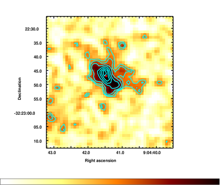
Figure 1: The X-ray image of the vicinity of T Pyx in the 0.3 to 9.0 keV range. The pixel resolution is 1^′′. North is up and West is to the right. The small red circle shows the location of the binary system. Overlaid are the X-ray contours with linear intensity increments.

Figure 2: The radial profiles of the source counts in the vicinity of T Pyx in three energy bands: 0.3-9.0 keV, top panel, 0.3-1.5 keV, middle panel, and 2.0-9.0 keV, bottom panel. The flat solid lines are the background. The source radial profiles are the data points indicated by unfilled squares and vertical error bars. The EPIC pn PSFs are indicated as curves with solid lines and are normalized to the counts in the first two radial bins of the profiles. A background is also added to the PSFs during the normalisation process. The resolution of spatial binning is 2^′′ for the top and middle panels and 1^′′ for the bottom panel with a few consecuitive bins averaged to improve statistics. The radial profiles and the corresponding EPIC pn PSFs are prepared using the SAS task ERADIAL.

3.2 The $XMM$-$Newton$ Spectrum of T Pyx

We performed spectral analysis of the EPIC data using the SAS task ESPECGET and derived the spectra of the source and the background together with the appropriate response matrices and ancillary files. How the photons were extracted is described in Section 2. The EPIC pn, EPIC MOS1 and EPIC MOS2 spectra were simultaneously fitted to derive spectral parameters of the emission arising from 15^′′ (radius of the circular photon exraction region) of the source position. The spectral analysis was performed using XSPEC version 12.5.1 (Arnaud 1996). A constant factor was included in the spectral fitting to allow for a normalisation uncertainty between the EPIC pn and EPIC MOS instruments. We grouped the pn and MOS spectral energy channels in groups of 100-150 to improve the statistical quality of the spectra. The fits were conducted in the 0.3-9.0 keV range. At first, we fitted a single blackbody or a composite model spectra where one component was a blackbody model to check the SSS scenario for the binary system. We find that the fits yield temperatures in excess of 1 keV as the best fit value which is inconsistent with the SSS scenario in accordance with the results of Selvelli et al. (2008). Next, assuming the emission is of the accretion shocks or the shocks in the nova ejecta, the three spectra were fitted with a single or two MEKAL emission models representing thermal plasma emission in collisional equilibrium (Liedahl, Osterheld & Goldstein 1995). For the intervening absorption ($N{\rm{}_{H}}$) we used the TBabs multiplicative model in XSPEC (Wilms, Allen & McCray 2000). The $N{\rm{}_{H}}$ was let to vary in order to account for any intrinsic absorption. All abundances were assumed at their solar values. We find that the best fits to the data using a single or two MEKAL models (TBabs*MEKAL or TBabs*(MEKAL+MEKAL)) yield unbounded plasma temperatures in excess of 70 keV with reduced $\chi^{2}$ values of 1.3-1.5. High shock temperatures may be achieved in accretion shocks, however we note that T Pyx is a non-magnetic CV and such systems show X-ray shock temperatures of 3-10 keV, in general (Baskill, Wheatly & Osborne 2005). Such high temperatures ($\sim$ 70 keV) are mostly achieved by some intermediate polars (a subclass of magnetic CVs) which T Pyx does not belong to (see Brunschweiger et al. 2009). We find that these fits are inconsistent with the accreting CV observations. Such high X-ray temperatures are also not in accordance with the hard X-ray observations of CNe/RNe (see the references in the Introduction). Furthermore, in the fitting process, we used some other plasma emission models like CEVMKL and MKCFLOW within the XSPEC software (instead of MEKAL model) that are largely used for the accreting CVs. The resulting X-ray temperatures are, also, unbounded and above 99 keV for CEVMKL and 21 keV-73 keV (lowT-highT) for MKCFLOW which are, also, inconsistent with CV observations. Finally, a successful fit was achieved using two different absorption components together with the two different temperature MEKAL models (TBabs*MEKAL+TBabs*MEKAL) with a reduced $\chi^{2}$ of 1.0 for 15 $d.o.f$ (degrees of freedom). Figure 3 shows the EPIC pn , EPIC MOS1 and EPIC MOS2 spectra fitted with this composite model. We derive for the first emission component an $N{\rm{}_{H1}}$ of 0.6${}^{+0.5}_{-0.4}$$\times 10^{22}$ cm^-2, $kT{\rm{}_{1}}$ of 0.2${}^{+0.7}_{-0.1}$ keV, and a normalisation of 2.9${}^{+168.0}_{-2.7}$$\times 10^{-4}$. The second emission component has an $N{\rm{}_{H2}}$ of 5.5${}^{+11.5}_{-4.0}$$\times 10^{22}$ cm^-2, $kT{\rm{}_{2}}$ of 1.3${}^{+1.0}_{-0.4}$ keV, and a normalisation of 4.5${}^{+9.3}_{-1.7}$$\times 10^{-4}$. Spectral uncertainties are given at 90% confidence level ($\Delta$$\chi^{2}$= 2.71 for a single parameter). The best fit results above indicate an absorbed X-ray flux of 2.3$\times 10^{-14}$ erg s^-1 cm^-2 and an unabsorbed X-ray flux of 3.7$\times 10^{-13}$ erg s^-1 cm^-2 which translates to an X-ray luminosity of 6.0$\times 10^{32}$ erg s^-1 at the source distance of 3.5 kpc (distance from Selvelli et al. 2008) in the energy range 0.3-10.0 keV. We also checked the existence of two spectral components by creating spectra in two annular photon extraction regions: (1) inner radius of 0^′′ and outer radius of 6^′′, and (2) inner radius of 7.5^′′ and outer radius of 15^′′ , centered on T Pyx. We find a similar spectrum to Figure 3 in the inner extraction region. However, the spectrum of the outer annulus shows only a 65$\%$ decrease in the emission below 1.5 keV and no emission above 1.5 keV. There is no need for a second harder X-ray spectral component.

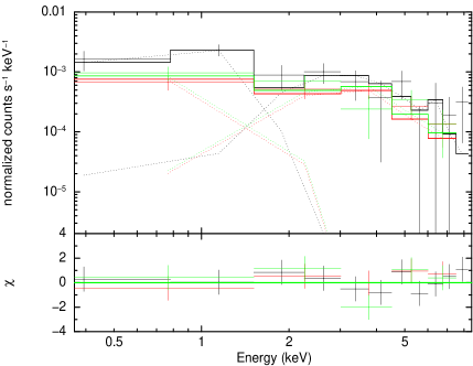
Figure 3: The $XMM$-$Newton$  EPIC data fitted with (TBabs*MEKAL + TBabs*MEKAL) model of emission in the 0.3-9.0 keV band. The red, green and black crosses indicate the EPIC MOS2, EPIC MOS1 and EPIC pn data, respectively. The dotted lines show the contribution of the two fitted MEKAL models. The lower panel shows the residuals between the data and the model in standard deviations.

4 Discussion

The spectrum of T Pyx is well described by two different plasmas in ionization equilibrium at different temperatures. We stress that the expected SSS is not detected and the radial profiles deviate significantly from the PSF of EPIC pn. If one assumes all the detected luminosity is due to accretion, this yields an accretion rate less than $<$ a few$\times$10^-10 M_⊙ yr^-1 for the system in contradiction with the optical and UV measurements by a factor of 10-100. This strengthens the possibility that most of the detected emission is of the nova remnant in the X-rays rather than the point source.

A simple shocked-shell model is of thermal origin. The total power from the shocked-shell, as an X-ray emitting nebula, can be expressed as in Balman (2005, 2006) $L_{x}\simeq 3.1\times 10^{33}T_{7}^{0.5}n_{o}^{2}R_{18.5}^{3}$. The temperature $T$ is in units of 10⁷ K and radius of the shell $R$ is in units of 3.1$\times 10^{18}$ cm. Using $R\sim 4.2\times 10^{17}$ cm, $n_{o}\sim$1-50 cm^-3 and $T\sim 10^{6.3-7.3}$ K, $L_{\rm x}$ is about 1.0$\times 10^{31}$-8.0$\times 10^{33}$ ergs s^-1. The detected X-ray luminosity (with $XMM$-$Newton$ ) is in this expected range of $L_{\rm x}$ for the shocked-shell emission. The detected emission measure $EM=<n_{e}>^{2}V_{eff}$ (calculated from normalisation of the fit) yields an average electron density $n_{e}$ of about 4.7 cm^-3 and 5.5 cm^-3 for the colder and hotter plasma, respectively, using a volume of 3.0$\times 10^{53}$ cm³ (consistent with a spherical region of 8^′′ radius at 3.5 kpc) and a filling factor f=1. If the filling factor is as low as 1$\times 10^{-4}$, then the electron density can be as high as 470-550 cm^-3 in the X-ray emitting region. The electron density calculated for the nova shell of GK Per is of similar order 0.6-11.0 cm^-3 for f=1 (Balman 2005). The spectrum of the nova remnant of GK Per also shows two plasma emission components with a significant difference of absorption between the two components (Balman 2005). Such differences can be explained by enhanced non-solar abundances of metals in cold material (possibly a shell or collection of dense knots) between the two emission components. A simple fit with the VARABS or VPHABS model (within XSPEC) using variable abundances for the second harder X-ray component yields an $N{\rm{}_{H2}}$ that is similar to $N{\rm{}_{H1}}$ within error ranges with enhanced abundances of N/N_⊙$\sim$ 20 and O/O_⊙$\sim$ 10 . The remnant of T Pyx shows strong [NII] emission, but the abundances of metals is unknown. The $N{\rm{}_{H}}$ difference can also be attributed to some complicated warm absorber effect (e.g. on the central binary system or the inner shell). Contini & Prialnik (1997) have modeled the circumstellar interaction of T Pyx shells. They find that as the latest shell catches the older shell, a forward shock moves into the older ejecta and a reverse shock moves into the new ejecta with typical electron densities of 100-300 cm^-3 and electron temperatures of about 0.1-0.9 keV. This model is very consistent with the X-ray spectral parameters obtained from the EPIC pn data (soft component).

The plasma temperatures of the two different MEKAL model components can be used to calculate the shock velocities using the general relation $kT_{s}=(3/16)\mu m_{H}(v_{s})^{2}$, ($T=1.4\times 10^{5}v^{2}_{\ 100kms^{-1}}$), assuming Rankine-Huguenot jump conditions in the absence of particle acceleration. We derive 400 km s^-1 (300-800 km s^-1 using error ranges) for the first plasma emission component and 1050 km s^-1 for the second more absorbed plasma emission component (maximum limit 1400 km s^-1 using error ranges). The shell expansion velocity is measured to be about 350-715 km s^-1 (Shara et al. 1989; Shara et al. 1997;O’Brien & Cohen 1998; Schaefer et al. 2010). This is consistent with the shock speeds calculated using the spectral parameters of the softer X-ray component. The radial profiles calculated from the $HST$ data require a multiple shell model with a particular shell found around 5^′′6^′′ and an extended emission region that goes out to 10^′′(both measured from the position of T Pyx; Shara et al. 1997; Schaefer et al. 2010). The [NII]+H${\alpha}$ images evidently shows an elongation/extension from the northeast to the southwest of the source position (see Figure 2c in Shara et al. 1989). The X-ray image indicates a similar elongation from the northeast to the southwest as well. This may be a result of the interaction between a bipolar outflow (e.g., a fast wind) during a RN outburst and the circumstellar environment (e.g., different shells) of the nova or the suggested CN remnant of 1866 by Schaefer et al. (2010). The expansion speeds of the 1966 outburst are in a range 850-2000 km s^-1 (Catchpole 1969). It has been about 40 years since the last outburst and the more absorbed (i.e. embeded) plasma emission component may belong to the most recent outburst. The expected location of the ejecta is about 2^′′ - 4^′′ (from the position of T Pyx). The expected size of the new interaction zone is within the core size of the EPIC pn PSF. The harder X-ray component may, also, belong to the binary system. A long observation of this source using the $Chandra$ Observatory (yielding better statistics) can resolve this issue with the aid of its superb pixel and PSF resolution.

References

- (1) Arnaud K. A., 1996, in ASP Conf. Ser. 101:Astronomical Data Analysis Software and Systems V, 17
- (2) Balman Ş., 2005, ApJ, 627, 933
- (3) —. 2006, Advances in Space Research, 38, 2840
- (4) Balman Ş., & Ögelman H. B., 1999, ApJ, 518, L111
- (5) Balman Ş., Krautter J., Ögelman, H., 1998, ApJ, 499, 395
- (6) Baskill D., Wheatley P.J., Osborne J.P., 2005, MNRAS, 357, 626
- (7) Bode M. F., Evans A., 2008, Classical Novae (Classical Novae, 2nd Edition. Edited by M.F. Bode and A. Evans. Cambridge Astrophysics Series, No. 43, Cambridge: Cambridge University Press, 2008.)
- (8) Bode M. F., et al. 2006, ApJ, 652, 629
- (9) Brunschweiger J,. Greiner J., Ajello M., Osborne J., 2009, A&A, 496, 121
- (10) Catchpole R. M., 1969, MNRAS, 142, 119
- (11) Contini M., Prialnik D., 1997, ApJ, 475, 803
- (12) Drake J. J. et al., 2009, ApJ, 691, 418
- (13) Ghizzardi S., 2002, XMMNewton Calibration Documentation (XMM-SOC-CAL-TN-0029)
- (14) Gilmozzi R., Selvelli P., 2007, A&A, 461, 593
- (15) Greiner J., Di Stefano R., 2002, ApJ, 578, L59
- (16) Hachisu I., Kato M., 2001, ApJ, 558, 323
- (17) Hernanz M., Sala G., 2002, Science, 298, 393
- (18) —. 2007, ApJ, 664, 467
- (19) Jansen F. et al., 2001, A&A, 365, L1
- (20) Krautter J., Ogelman H., Starrfield S., Wichmann, R., Pfeffermann J., 1996, ApJ, 456, 788
- (21) Liedahl D. A., Osterheld A. L., Goldstein W. H., 1995, ApJ, 438, L115
- (22) Livio M. 1994, in Interacting Binaries, Saas-Fee Advanced Course 22, ed. H. Nussbaumer, A. Orr (Berlin: Springer), 135
- (23) Luna G.J., Montez R., Sokoloski J.L., Mukai K., Kastner J.H., 2009, ApJ, 707, L1168
- (24) Mukai K., Ishida M., 2001, ApJ, 551, 1024
- (25) Ness J.-U. et al., 2009, AJ, 137, 3414
- (26) Ness J.-U. et al., 2003, ApJ, 594, L127
- (27) O’Brien T. J., Lloyd H. M., Bode M. F., 1994, MNRAS, 271, 155
- (28) O’Brien T. J., Cohen J. G., 1998, ApJ, 498, L59
- (29) Orio M. et al., 2001, MNRAS, 326, L13
- (30) Orio M., Tepedelenlioglu E., Starrfield S., Woodward C. E., Della Valle M., 2005, ApJ, 620, 938
- (31) Pekön Y., Balman, Ş., 2008, MNRAS, 388, 921
- (32) Page K.L. et al., 2009, A&A, 507, 923
- (33) Patterson P. et al., 1998, PASP, 110, 380
- (34) Prialnik D., Kovetz A., 1995, ApJ, 445, 789
- (35) Schaefer B. E., Pagnotta A., Shara M. M., 2010, ApJ, 708, 381
- (36) Selvelli P., Cassatella A., Gilmozzi R., González-Riestra R., 2008, A&A, 492, 787
- (37) Shara M. M., 1989, PASP, 101, 5
- (38) Shara M. M., Zurek D. R., Williams R. E., Prialnik D., Gilmozzi R., Moffat A. F. J., 1997, AJ, 114, 258
- (39) Sokoloski J. L., Luna G. J. M., Mukai K., Kenyon S. J., 2006, Nature, 442, 276
- (40) Starrfield S., Sparks W. M., Truran J. W., 1985, ApJ, 291, 136
- (41) Strüder L. et al., 2001, A&A, 365, L18
- (42) Turner M. J. L. et al., 2001, A&A, 365, L27
- (43) Webbink R. F., Livio M., Truran J. W., Orio M., 1987, Ap&SS, 131, 493
- (44) Wilms J., Allen A., McCray R., 2000, ApJ, 542, 914
- (45) Yaron O., Prialnik D., Shara M. M., Kovetz A., 2005, ApJ, 623, 398