Abstract

Following Hartigan (1975), a cluster is defined as a connected component of the $t$-level set of the underlying density, i.e., the set of points for which the density is greater than $t$. A clustering algorithm which combines a density estimate with spectral clustering techniques is proposed. Our algorithm is composed of two steps. First, a nonparametric density estimate is used to extract the data points for which the estimated density takes a value greater than $t$. Next, the extracted points are clustered based on the eigenvectors of a graph Laplacian matrix. Under mild assumptions, we prove the almost sure convergence in operator norm of the empirical graph Laplacian operator associated with the algorithm. Furthermore, we give the typical behavior of the representation of the dataset into the feature space, which establishes the strong consistency of our proposed algorithm.

Index Terms: Spectral clustering, graph, unsupervised classification, level sets, connected components.

1 Introduction

The aim of data clustering, or unsupervised classification, is to partition a data set into several homogeneous groups relatively separated one from each other with respect to a certain distance or notion of similarity. There exists an extensive literature on clustering methods, and we refer the reader to Anderberg (1973); Hartigan (1975); McLachlan and Peel (2000), Chapter 10 in Duda et al. (2000), and Chapter 14 in Hastie et al. (2001) for general materials on the subject. In particular, popular clustering algorithms, such as Gaussian mixture models or k-means, have proved useful in a number of applications, yet they suffer from some internal and computational limitations. Indeed, the parametric assumption at the core of mixture models may be too stringent, while the standard k-means algorithm fails at identifying complex shaped, possibly non-convex, clusters.

The class of spectral clustering algorithms is presently emerging as a promising alternative, showing improved performance over classical clustering algorithms on several benchmark problems and applications; see e.g., Ng et al. (2002); von Luxburg (2007). An overview of spectral clustering algorithms may be found in von Luxburg (2007), and connections with kernel methods are exposed in Fillipone et al. (2008). The spectral clustering algorithm amounts at embedding the data into a feature space by using the eigenvectors of the similarity matrix in such a way that the clusters may be separated using simple rules, e.g. a separation by hyperplanes. The core component of the spectral clustering algorithm is therefore the similarity matrix, or certain normalizations of it, generally called graph Laplacian matrices; see Chung (1997). Graph Laplacian matrices may be viewed as discrete versions of bounded operators between functional spaces. The study of these operators has started out recently with the works by Belkin et al. (2004); Belkin and Niyogi (2005); Coifman and Lafon (2006); Nadler et al. (2006); Koltchinskii (1998); Giné and Koltchinskii (2006); Hein et al. (2007), among others, and the convergence of the spectral clustering algorithm has been established in von Luxburg et al. (2008).

The standard k-means clustering leads to the optimal quantizer of the underlying distribution; see MacQueen (1967); Pollard (1981); Linder (2002). However, determining what the limit clustering obtained in von Luxburg et al. (2008) represents for the distribution of the data remains largely an open question. As a matter of fact, there exists many definitions of a cluster; see e.g., von Luxburg and Ben-David (2005) or García-Escudero et al. (2008). Perhaps the most intuitive and precise definition of a cluster is the one introduced by Hartigan (1975). Suppose that the data is drawn from a probability density $f$ on $\mathbb{R}^{d}$ and let $t$ be a positive number in the range of $f$. Then a cluster in the sense of Hartigan (1975) is a connected component of the $t$-level set

$$\mathcal{L}(t)=\big{\{}x\in\mathbb{R}^{d}\,:\,f(x)\geq t\big{\}}.$$

This definition has several advantages. First, it is geometrically simple. Second, it offers the possibility of filtering out possibly meaningless clusters by keeping only the observations falling in a region of high density, This proves useful, for instance, in the situation where the data exhibits a cluster structure but is contaminated by a uniform background noise, as illustrated in our simulations in Section 4.

In this context, the level $t$ should be considered as a resolution level for the data analysis. Several clustering algorithms have been introduced building upon Hartigan’s definition. In Cuevas et al. (2000, 2001), clustering is performed by estimating the connected components of $\mathcal{L}(t)$; see also the work by Azzalini and Torelli (2007). Hartigan’s definition is also used in Biau et al. (2007) to define an estimate of the number of clusters.

In the present paper, the definition of a cluster given by Hartigan (1975) is adopted, and we introduce a spectral clustering algorithm on estimated level sets. More precisely, given a random sample $X_{1},\dots,X_{n}$ drawn from a density $f$ on $\mathbb{R}^{d}$, our proposed algorithm is composed of two operations. In the first step, given a positive number $t$, we extract the observations for which $\hat{f}_{n}(X_{i})\geq t$, where $\hat{f}_{n}$ is a nonparametric density estimate of $f$ based on the sample $X_{1},\dots,X_{n}$. In the second step, we perform a spectral clustering of the extracted points. The remaining data points are then left unlabeled.

Our proposal is to study the asymptotic behavior of this algorithm. As mentioned above, strong interest has recently been shown in spectral clustering algorithms, and the major contribution to the proof of the convergence of spectral clustering is certainly due to von Luxburg et al. (2008). In von Luxburg et al. (2008), the graph Laplacian matrix is associated with some random operator acting on the Banach space of continuous functions. They prove the collectively compact convergence of those operators towards a limit operator. Under mild assumptions, we strengthen their results by establishing the almost sure convergence in operator norm, but in a smaller Banach space (Theorem 3.1). This operator norm convergence is more amenable than the slightly weaker notion of convergence established in von Luxburg et al. (2008). For instance, it is easy to check that the limit operator, and the graph Laplacian matrices used in the algorithm, are continuous in the scale parameter $h$.

We also derive the asymptotic representation of the dataset in the feature space in Corollary 3.2. This result implies that the proposed algorithm is strongly consistent and that, asymptotically, observations of $\mathcal{L}(t)$ are assigned to the same cluster if and only if they fall in the same connected component of the level set $\mathcal{L}(t)$.

The paper is organized as follows. In Section 2, we introduce some notations and assumptions, as well as our proposed algorithm. Section 3 contains our main results, namely the convergence in operator norm of the random operators, and the characterization of the dataset embedded into the feature space. We provide a numerical example with a simulated dataset in Section 4. Sections 5 and 6 are devoted to the proofs. At the end of the paper, a technical result on the geometry of level sets is stated in Appendix A, some useful results of functional analysis are summarized in Appendix B, and the theoretical properties of the limit operator are given in Appendix C.

2 Spectral clustering algorithm

2.1 Mathematical setting and assumptions

Let $\{X_{i}\}_{i\geq 1}$ be a sequence of i.i.d. random vectors in $\mathbb{R}^{d}$, with common probability measure $\mu$. Suppose that $\mu$ admits a density $f$ with respect to the Lebesgue measure on $\mathbb{R}^{d}$. The $t$-level set of $f$ is denoted by $\mathcal{L}(t)$, i.e.,

$$\mathcal{L}(t)=\big{\{}x\in\mathbb{R}^{d}\,:\,f(x)\geq t\big{\}},$$

for all positive level $t$, and given $a\leq b$, $\mathcal{L}_{a}^{b}$ denotes the set $\{x\in\mathbb{R}^{d}\,:\,a\leq f(x)\leq b\}$. The differentiation operator with respect to $x$ is denoted by $D_{x}$. We assume that $f$ satisfies the following conditions.

Assumption 1. (i) $f$ is of class $\mathcal{C}^{2}$ on $\mathbb{R}^{d}$; (ii) $\|D_{x}f\|>0$ on the set $\{x\in\mathbb{R}^{d}\,:\,f(x)=t\}$; (iii) $f$, $D_{x}f$, and $D^{2}_{x}f$ are uniformly bounded on $\mathbb{R}^{d}$.

Note that under Assumption 1, $\mathcal{L}(t)$ is compact whenever $t$ belongs to the interior of the range of $f$. Moreover, $\mathcal{L}(t)$ has a finite number $\ell$ of connected components ${\mathcal{C}}_{j}$, $j=1,\ldots,\ell$. For ease of notation, the dependence of $\mathcal{C}_{j}$ on $t$ is omitted. The minimal distance between the connected components of $\mathcal{L}(t)$ is denoted by $d_{min}$, i.e.,

$$d_{min}=\inf_{i\neq j}{\rm dist}\big{(}\mathcal{C}_{i},\mathcal{C}_{j}\big{)}.$$ (2.1)

Let $\widehat{f}_{n}$ be a consistent density estimate of $f$ based on the random sample $X_{1},\dots,X_{n}$. The $t$-level set of $\widehat{f}_{n}$ is denoted by $\mathcal{L}_{n}(t)$, i.e.,

$$\mathcal{L}_{n}(t)=\big{\{}x\in\mathbb{R}^{d}\,:\,\widehat{f}_{n}(x)\geq t\big{\}}.$$

Let $J(n)$ be the set of integers defined by

$$J(n)=\big{\{}j\in\{1,\dots,n\}:\,\widehat{f}_{n}(X_{j})\geq t\big{\}}.$$

The cardinality of $J(n)$ is denoted by $j(n)$.

Let $k:\mathbb{R}^{d}\to\mathbb{R}_{+}$ be a fixed function. The unit ball of $\mathbb{R}^{d}$ centered at the origin is denoted by $B$, and the ball centered at $x\in\mathbb{R}^{d}$ and of radius $r$ is denoted by $x+rB$. We assume throughout that the function $k$ satisfies the following set of conditions.

Assumption 2. (i) $k$ is of class $\mathcal{C}^{2}$ on $\mathbb{R}^{d}$; (ii) the support of $k$ is $B$; (iii) $k$ is uniformly bounded from below on $B/2$ by some positive number; and (iv) $k(-x)=k(x)$ for all $x\in\mathbb{R}^{d}$.

Let $h$ be a positive number. We denote by $k_{h}:\mathbb{R}^{d}\to\mathbb{R}_{+}$ the map defined by $k_{h}(u)=k({u}/{h})$.

2.2 Algorithm

The first ingredient of our algorithm is the similarity matrix $\mathbf{K}_{n,h}$ whose elements are given by

$$\mathbf{K}_{n,h}(i,j)=k_{h}(X_{j}-X_{i}),$$

and where the integers $i$ and $j$ range over the random set $J(n)$. Hence $\mathbf{K}_{n,h}$ is a random matrix indexed by $J(n)\times J(n)$, whose values depend on the function $k_{h}$, and on the observations $X_{j}$ lying in the estimated level set $\mathcal{L}_{n}(t)$. Next, we introduce the diagonal normalization matrix $\mathbf{D}_{n,h}$ whose diagonal entries are given by

$$\mathbf{D}_{n,h}(i,i)=\sum_{j\in J(n)}\mathbf{K}_{n,h}(i,j),\quad i\in J(n).$$

Note that the diagonal elements of $\mathbf{D}_{n,h}$ are positive.

The spectral clustering algorithm is based on the matrix $\mathbf{Q}_{n,h}$ defined by

$$\mathbf{Q}_{n,h}=\mathbf{D}_{n,h}^{-1}\mathbf{K}_{n,h}.$$

Observe that $\mathbf{Q}_{n,h}$ is a random Markovian transition matrix. Note also that the (random) eigenvalues of $\mathbf{Q}_{n,h}$ are real numbers and that $\mathbf{Q}_{n,h}$ is diagonalizable. Indeed the matrix $\mathbf{Q}_{n,h}$ is conjugate to the symmetric matrix $\mathbf{S}_{n,h}:=\mathbf{D}_{n,h}^{-1/2}\mathbf{K}_{n,h}\mathbf{D}_{n,h}^{-1/2}$ since we may write

$$\mathbf{Q}_{n,h}=\mathbf{D}_{n,h}^{-1/2}\mathbf{S}_{n,h}\mathbf{D}_{n,h}^{1/2}.$$

Moreover, the inequality $\|\mathbf{Q}_{n,h}\|_{\infty}\leq 1$ implies that the spectrum $\sigma(\mathbf{Q}_{n,h})$ is a subset of $[-1;+1]$. Let $1=\lambda_{n,1}\geq\lambda_{n,2}\geq\ldots\geq\lambda_{n,j(n)}\geq-1$ be the eigenvalues of $\mathbf{Q}_{n,h}$, where in this enumeration, an eigenvalue is repeated as many times as its multiplicity.

To implement the spectral clustering algorithm, the data points of the partitioning problem are first embedded into $\mathbb{R}^{\ell}$ by using the eigenvectors of $\mathbf{Q}_{n,h}$ associated with the $\ell$ largest eigenvalues, namely $\lambda_{n,1}$, $\lambda_{n,2}$, …$\lambda_{n,\ell}$. More precisely, fix a collection $V_{n,1}$, $V_{n,2}$, …, $V_{n,\ell}$ of such eigenvectors with components respectively given by $V_{n,k}=\{V_{n,k,j}\}_{j\in J(n)}$, for $k=1,\dots,\ell$. Then the $j^{\rm th}$ data point, for $j$ in $J(n)$, is represented by the vector $\rho_{n}({X}_{j})$ of $\mathbb{R}^{\ell}$ defined by $\rho_{n}({X}_{j}):=\{V_{n,k,j}\}_{1\leq k\leq\ell}$. At last, the embedded points are partitioned using a classical clustering method, such as the k-means algorithm for instance.

2.3 Functional operators associated with the matrices of the algorithm

As exposed in the Introduction, some functional operators are associated with the matrices acting on $\mathbb{C}^{J(n)}$ defined in the previous paragraph. The link between matrices and functional operators is provided by the evaluation map defined in (2.3) below. As a consequence, asymptotic results on the clustering algorithm may be derived by studying first the limit behavior of these operators.

To this aim, let us first introduce some additional notation. For $\mathcal{D}$ a subset of $\mathbb{R}^{d}$, let $W(\mathcal{D})$ be the Banach space of complex-valued, bounded, and continuously differentiable functions with bounded gradient, endowed with the norm

$$\|g\|_{W}=\|g\|_{\infty}+\|D_{x}g\|_{\infty}.$$

Consider the non-oriented graph whose vertices are the $X_{j}$’s for $j$ ranging in $J(n)$. The similarity matrix $\mathbf{K}_{n,h}$ gives random weights to the edges of the graph and the random transition matrix $\mathbf{Q}_{n,h}$ defines a random walk on the vertices of a random graph. Associated with this random walk is the transition operator $Q_{n,h}:W\big{(}\mathcal{L}_{n}(t)\big{)}\to W\big{(}\mathcal{L}_{n}(t)\big{)}$ defined for any function $g$ by

$$Q_{n,h}g(x)=\int_{\mathcal{L}_{n}(t)}q_{n,h}(x,y)g(y)\mathbb{P}_{n}^{t}(dy).$$

In this equation, $\mathbb{P}_{n}^{t}$ is the discrete random probability measure given by

$$\mathbb{P}_{n}^{t}=\frac{1}{j(n)}\sum_{j\in J(n)}\delta_{X_{j}},$$

and

$$q_{n,h}(x,y)=\frac{k_{h}(y-x)}{K_{n,h}(x)},\quad\mathrm{where}~{}K_{n,h}(x)=\int_{\mathcal{L}_{n}(t)}k_{h}(y-x)\mathbb{P}_{n}^{t}(dy).$$ (2.2)

In the definition of $q_{n,h}$, we use the convention that $0/0=0$, but this situation does not occur in the proofs of our results.

Given the evaluation map $\pi_{n}:{W}\big{(}\mathcal{L}_{n}(t)\big{)}\to\mathbb{C}^{J(n)}$ defined by

$$\pi_{n}(g)=\Big{\{}g(X_{j})\,:\,j\in J(n)\Big{\}},$$ (2.3)

the matrix $\mathbf{Q}_{n,h}$ and the operator $Q_{n,h}$ are related by $\mathbf{Q}_{n,h}\circ\pi_{n}=\pi_{n}\circ Q_{n,h}$. Using this relation, asymptotic properties of the spectral clustering algorithm may be deduced from the limit behavior of the sequence of operators $\{Q_{n,h}\}_{n}$. The difficulty, though, is that $Q_{n,h}$ acts on ${W}\big{(}\mathcal{L}_{n}(t)\big{)}$ and $\mathcal{L}_{n}(t)$ is a random set which varies with the sample. For this reason, we introduce a sequence of operators $\widehat{Q}_{n,h}$ acting on $W\big{(}\mathcal{L}(t)\big{)}$ and constructed from $Q_{n,h}$ as follows.

First of all, recall that under Assumption 1, the gradient of $f$ does not vanish on the set $\{x\in\mathbb{R}^{d}\,:\,f(x)=t\}$. Since $f$ is of class $\mathcal{C}^{2}$, a continuity argument implies that there exists $\varepsilon_{0}>0$ such that $\mathcal{L}_{t-\varepsilon_{0}}^{t+\varepsilon_{0}}$ contains no critical points of $f$. Under this condition, Lemma A.1 states that $\mathcal{L}(t+\varepsilon)$ is diffeomorphic to $\mathcal{L}(t)$ for every $\varepsilon$ such that $|\varepsilon|\leq\varepsilon_{0}$. In all of the following, it is assumed that $\varepsilon_{0}$ is small enough so that

$$\varepsilon_{0}/\alpha(\varepsilon_{0})<h/2,\quad\text{where}~{}\alpha(\varepsilon_{0})=\inf\big{\{}\|D_{x}f(x)\|;\,x\in\mathcal{L}_{t-\varepsilon_{0}}^{t}\big{\}}.$$ (2.4)

Let $\{\varepsilon_{n}\}_{n}$ be a sequence of positive numbers such that $\varepsilon_{n}\leq\varepsilon_{0}$ for each $n$, and $\varepsilon_{n}\to 0$ as $n\to\infty$. In Lemma A.1 an explicit diffeomorphism $\varphi_{n}$ carrying $\mathcal{L}(t)$ to $\mathcal{L}(t-\varepsilon_{n})$ is constructed, i.e.,

$$\varphi_{n}:\mathcal{L}(t)\stackrel{{\scriptstyle\cong}}{{\longrightarrow}}\mathcal{L}(t-\varepsilon_{n}).$$ (2.5)

The diffeomorphism $\varphi_{n}$ induces the linear operator $\Phi_{n}:W\big{(}\mathcal{L}(t)\big{)}\to W\big{(}\mathcal{L}(t-\varepsilon_{n})\big{)}$ defined by $\Phi_{n}g=g\circ\varphi_{n}^{-1}.$

Second, let $\Omega_{n}$ be the probability event defined by

$$\Omega_{n}=\Big{[}\|\widehat{f}_{n}-f\|_{\infty}\leq\varepsilon_{n}\Big{]}\cap\left[\inf\left\{\|D_{x}\widehat{f}_{n}(x)\|,x\in{\mathcal{L}_{t-\varepsilon_{0}}^{t+\varepsilon_{0}}}\right\}\geq\frac{1}{2}\|D_{x}f\|_{\infty}\right].$$ (2.6)

Note that on the event $\Omega_{n}$, the following inclusions hold:

$$\mathcal{L}(t-\varepsilon_{n})\subset\mathcal{L}_{n}(t)\subset\mathcal{L}(t+\varepsilon_{n}).$$ (2.7)

We assume that the indicator function $\mathbf{1}_{\Omega_{n}}$ tends to $1$ almost surely as $n\to\infty$, which is satisfied by common density estimates $\widehat{f}_{n}$ under mild assumptions. For instance, consider a kernel density estimate with a Gaussian kernel. Then for a density $f$ satisfying the conditions in Assumption 1, we have $\|D_{x}^{(p)}\widehat{f}_{n}-D_{x}^{(p)}f\|_{\infty}\to 0$ almost surely as $n\to\infty$, for $p=0$ and $p=1$ (see e.g., Prakasa Rao (1983)), which implies that $\mathbf{1}_{\Omega_{n}}\to 1$ almost surely as $n\to\infty$.

We are now in a position to introduce the operator $\widehat{Q}_{n,h}:W\big{(}\mathcal{L}(t)\big{)}\to W\big{(}\mathcal{L}(t)\big{)}$ defined on the event $\Omega_{n}$ by

$$\widehat{Q}_{n,h}=\Phi_{n}^{-1}Q_{n,h}\Phi_{n},$$ (2.8)

and we extend the definition of $\widehat{Q}_{n,h}$ to the whole probability space by setting it to the null operator on the complement $\Omega_{n}^{c}$ of $\Omega_{n}$. In other words, on $\Omega_{n}^{c}$, the function $\widehat{Q}_{n,h}g$ is identically zero for each $g\in W\big{(}\mathcal{L}(t)\big{)}$.

Remark 2.1.

Albeit the relevant part of $\widehat{Q}_{n,h}$ is defined on $\Omega_{n}$ for technical reasons, this does not bring any difficulty as long as one is concerned with almost sure convergence. To see this, let $(\Omega,\mathcal{A},P)$ be the probability space on which the $X_{i}$’s are defined. Denote by $\Omega_{\infty}$ the event on which $\mathbf{1}_{\Omega_{n}}$ tends to 1, and recall that $P(\Omega_{\infty})=1$ by assumption. Thus, for every $\omega\in\Omega$, there exists a random integer $n_{0}(\omega)$ such that, for each $n\geq n_{0}(\omega)$, $\omega$ lies in $\Omega_{n}$. Besides $n_{0}(\omega)$ is finite on $\Omega_{\infty}$. Hence in particular, if $\{Z_{n}\}$ is a sequence of random variables such that $Z_{n}\mathbf{1}_{\Omega_{n}}$ converges almost surely to some random variable $Z_{\infty}$, then $Z_{n}\to Z_{\infty}$ almost surely.

3 Main results

Our main result (Theorem 3.1) states that $\widehat{Q}_{n,h}$ converges in operator norm to the limit operator $Q_{h}:W\big{(}\mathcal{L}(t)\big{)}\to W\big{(}\mathcal{L}(t)\big{)}$ defined by

$$Q_{h}g(x)=\int_{\mathcal{L}(t)}q_{h}(x,y)g(y)\mu^{t}(dy),$$ (3.1)

where $\mu^{t}$ denotes the conditional distribution of $X$ given the event $\big{[}X\in\mathcal{L}(t)\big{]}$, and where

$$q_{h}(x,y)=\frac{k_{h}(y-x)}{K_{h}(x)},\quad\mathrm{with}~{}K_{h}(x)=\int_{\mathcal{L}(t)}k_{h}(y-x)\mu^{t}(dy).$$ (3.2)

Theorem 3.1 (Operator Norm Convergence).

Suppose that Assumptions 1 and 2 hold. We have

$$\big{\|}\widehat{Q}_{n,h}-Q_{h}\big{\|}_{W}\to 0\quad\text{almost surely as }n\to\infty.$$

The proof of Theorem 3.1 is given in Paragraph 5.2. Its main arguments are as follows. First, the three classes of functions defined in Lemma 5.2 are shown to be Glivenko-Cantelli. This, together with additional technical results, leads to uniform convergences of some linear operators (Lemma 5.6).

Theorem 3.1 implies the consistency of our algorithm. We recall that $d_{min}$ given in (2.1) is the minimal distance between the connected components of the level set. The starting point is the fact that, provided that $h<d_{\text{min}}$, the connected components of the level set $\mathcal{L}(t)$ are the recurrent classes of the Markov chain whose transitions are given by $Q_{h}$. Indeed, this process cannot jump from one component to the other ones. Hence, $Q_{h}$ defines the desired clustering via its eigenspace corresponding to the eigenvalue $1$.

As stated in Proposition C.2 in the Appendices, the eigenspace of the limit operator $Q_{h}$ associated with the eigenvalue $1$ is spanned by the indicator functions of the connected components of $\mathcal{L}(t)$. Hence the representation of the extracted part of the dataset into the feature space $\mathbb{R}^{\ell}$ (see the end of Paragraph 2.2) tends to concentrate around $\ell$ different centroids. Moreover, each of these centroids corresponds to a cluster, i.e., to a connected component of $\mathcal{L}(t)$.

More precisely, using the convergence in operator norm of $\widehat{Q}_{n,h}$ towards $Q_{h}$, together with the results of functional analysis given in Appendix B, we obtain the following corollary which describes the asymptotic behavior of our algorithm. Let us denote by $J(\infty)$ the set of integers $j$ such that $X_{j}$ is in the level set $\mathcal{L}(t)$. For all $j\in J(\infty)$, define $k(j)$ as the integer such that $X_{j}\in\mathcal{C}_{k(j)}$.

Corollary 3.2.

Suppose that Assumptions 1 and 2 hold, and that $h$ is in $(0;d_{min})$. There exists a sequence $\{\xi_{n}\}_{n}$ of linear transformations of $\mathbb{R}^{\ell}$ such that, for all $j\in J(\infty)$, $\xi_{n}\rho_{n}(X_{j})$ converges almost surely to $e_{k(j)}$, where $e_{k(j)}$ is the vector of $\mathbb{R}^{\ell}$ whose components are all 0 except the $k(j)^{\rm th}$ component equal to $1$.

Corollary 3.2, which is new up to our knowledge, is proved in Section 6. Corollary 3.2 states that the data points embedded in the feature space concentrate on separated centroids. As a consequence, any partitioning algorithm (e.g., $k$-means) applied in the feature space will asymptotically yield the desired clustering. In other words, the clustering algorithm is consistent. Note that if one is only interested in the consistency property, then this result could be obtained through another route. Indeed, it is shown in Biau et al. (2007) that the neighborhood graph with connectivity radius $h$ has asymptotically the same number of connected components as the level set. Hence, splitting the graph into its connected components leads to the desired clustering as well. But Corollary 3.2, by giving the asymptotic representation of the data when embedded in the feature space $\mathbb{R}^{\ell}$, provides additional insight into spectral clustering algorithms. In particular, Corollary 3.2 provides a rationale for the heuristic of Zelnik-Manor and Perona (2004) for automatic selection of the number of groups. Their idea is to quantify the amount of concentration of the points embedded in the feature space, and to select the number of groups leading to the maximal concentration. Their method compared favorably with the eigengap heuristic considered in von Luxburg (2007).

Naturally, the selection of the number of groups is also linked with the choice of the parameter $h$. In this direction, let us emphasize that the operators $\widehat{Q}_{n,h}$ and $Q_{h}$ depend continuously on the scale parameter $h$. Thus, the spectral properties of both operators will be close to the ones stated in Corollary 3.2, if $h$ is in the neighborhood of the interval $(0;d_{min})$. This follows from the continuity of an isolated set of eigenvalues, as stated in Appendix B. In particular, the sum of the eigenspaces of $Q_{h}$ associated with the eigenvalues close to $1$ is spanned by functions that are close to (in $W(\mathcal{L}(t))$-norm) the indicator functions of the connected components of $\mathcal{L}(t)$. Hence, the representation of the dataset in the feature space $\mathbb{R}^{\ell}$ still concentrates on some neighborhoods of $e_{k}$, $1\leq k\leq\ell$ and a simple clustering algorithm such as $k$-means will still give the desired result. To sum up the above, if assumptions 1 and 2 hold, our algorithm is consistent for all $h$ in $(0,h_{max})$ for some $h_{max}>d_{min}$.

Several questions, though, remain largely open. For instance, one might ask if a similar result holds for the classical spectral clustering algorithm, i.e., without the preprocessing step. This case corresponds to taking $t=0$. One possibility may then be to consider a sequence $h_{n}$, with $\lim h_{n}=0$ and to the study the limit of the operator $Q_{n,h_{n}}$.

4 Simulations

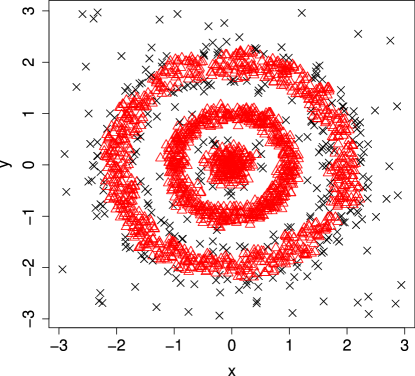
Figure 1: Left: simulated points. Right: Points belonging to the estimated level set (red triangle) and remaining points (dark cross).

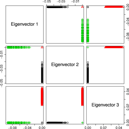
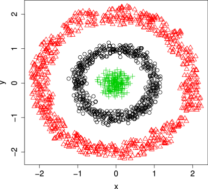
Figure 2: Top Left: first 10 eigenvalues, sorted in ascending order. Top Right: pairs plots of the first three eigenvectors. It may be seen that the embedded data concentrate around three distinct points in the feature space $\mathbb{R}^{3}$. Bottom Resulting partition obtained by applying a $k$-means algorithm in the feature space. The color scheme is identical to the representation of the eigenvectors (top-right panel). The three groups are accurately recovered.

Figure 3: First 50 eigenvalues of the standard spectral clustering algorithm, applied on the initial data set, i.e., without level set pre-processing. A total of 35 eigenvalues are found equal to zero, which leads to 35 inhomogeneous groups, indicating failure of the standard spectral clustering algorithm.

We consider a mixture density on $\mathbb{R}^{2}$ with four components corresponding to random variables $X_{1},\dots,X_{4}$ where

• $X_{1}\sim\mathcal{N}(0,\sigma_{1}^{2}\mathbf{I})$ with $\sigma_{1}=0.2$ ;

• $X_{2}=R_{2}(\cos\theta_{2},\sin\theta_{2})$ where $\theta_{2}\sim\mathcal{U}([0;2\pi])$ and $R_{2}\sim\mathcal{N}(1,0.1^{2})$ ;

• $X_{3}=R_{3}(\cos\theta_{3},\sin\theta_{3})$ where $\theta_{3}\sim\mathcal{U}([0;2\pi])$ and $R_{3}\sim\mathcal{N}(2,0.2^{2})$ ;

• $X_{4}\sim\mathcal{U}([-3;3]\times[-3;3])$.

The proportions of the components in the mixture are taken as $10\%$, $32\%$, $53\%$ and $5\%$, respectively. The fourth component ($X_{4}$) represents a uniform background noise.

A random sample of size $n=1,900$ has been simulated according to the mixture. Points are displayed in Figure 1 (left). A nonparametric kernel density estimate, with a Gaussian kernel, has been adjusted to the data. The bandwidth parameter of the density estimate has been selected automatically with cross-validation. A level $t=0.0444$ has been selected such that $85\%$ of the simulated points are extracted, i.e., $85\%$ of the observations fall in $\mathcal{L}_{n}(t)$. The extracted and discarded points are displayed in Figure 1 (right). The number of extracted points is equal to $1,615$.

The spectral clustering has been applied to the $1,615$ extracted points, with the similarity function

$$k(x)=\exp(-1/(1-\|x\|)^{2})\mathbf{1}\{\|x\|<1\}.$$

For numerical stability of the algorithm, we considered the eigendecomposition of the symmetric matrix $\mathbf{I}-\mathbf{S}_{n,h}$. Thus, the eigenspace associated with the eigenvalue $1$ of the matrix $\mathbf{Q}_{n,h}$ corresponds to the null space of $\mathbf{I}-\mathbf{S}_{n,h}$. The scale parameter $h$ has be empirically chosen equal to $0.25$. The first 10 eigenvalues of $\mathbf{I}-\mathbf{S}_{n,h}$ are represented in Figure 2 (top-left). Three eigenvalues are found equal to zero, indicating three distinct groups. The data is then embedded in $\mathbb{R}^{3}$ using the three eigenvectors of the null space of $\mathbf{I}-\mathbf{S}_{n,h}$, and the data is partitioned in this space using a $k$-means clustering algorithm. Pair plots of three eigenvectors of the null space are displayed in Figure 2. It may be observed that the embedded data are concentrated around three distinct points in the feature space. Applying a $k$-means algorithm in the feature space leads to the partition represented in Figure 2. Note that observations considered as background noise are the discarded points belonging to the complement of $\mathcal{L}_{n}(t)$. In this example, our algorithm is successful at recovering the three expected groups.

As a comparison, we applied the standard spectral clustering algorithm to the initial data set of size $n=1,900$. In this case, $35$ eigenvalues are found equal to zero (Figure 3). Applying a $k$-means clustering algorithm in the embedding space $\mathbb{R}^{35}$ leads to 35 inhomogeneous groups (not displayed here), none of which corresponds roughly to the expected groups (the two circular bands and the inner circle). This failure of the standard spectral clustering algorithm is explained by the presence of the background noise which, when unfiltered, perturbs the formation of distinct groups. While there remains multiple important questions, in particular regarding the choice of the parameter $h$, these simulations illustrate the added value of combining a spectral clustering algorithm with level-set techniques.

5 Proof of the convergence of $\widehat{Q}_{n,h}$ (Theorem 3.1)

5.1 Preliminaries

Let us start with the following simple lemma.

Lemma 5.1.

Let $\{A_{n}\}_{n\geq 0}$ be a decreasing sequence of Borel sets in $\mathbb{R}^{d}$, with limit $A_{\infty}=\cap_{n\geq 0}A_{n}$. If $\mu(A_{\infty})=0$, then

$$\mathbb{P}_{n}A_{n}=\frac{1}{n}\sum_{i=1}^{n}\mathbf{1}\{X_{i}\in A_{n}\}\to 0\quad\text{almost surely as $n\to\infty$,}$$

where $\mathbb{P}_{n}$ is the empirical measure associated with the random sample $X_{1},\dots,X_{n}$.

Proof. First, note that $\lim_{n}\mu(A_{n})=\mu(A_{\infty})$. Next, fix an integer $k$. For all $n\geq k$, $A_{n}\subset A_{k}$ and so $\mathbb{P}_{n}A_{n}\leq\mathbb{P}_{n}A_{k}$. But $\lim_{n}\mathbb{P}_{n}A_{k}=\mu(A_{k})$ almost surely by the law of large numbers. Consequently $\limsup_{n}\mathbb{P}_{n}A_{n}\leq\mu(A_{k})$ almost surely. Letting $k\to\infty$ yields

$$\limsup_{n}\mathbb{P}_{n}A_{n}\leq\mu(A_{\infty})=0,$$

which concludes the proof since $\mathbb{P}_{n}A_{n}\geq 0$. $\Box$

The operator norm convergence that we expect to prove is a uniform law of large number. The key argument is the fact that the classes of functions of the following lemma are Glivenko-Cantelli. Let $g$ be a function defined on some subset $\mathcal{D}$ of $\mathbb{R}^{d}$, and let $\mathcal{A}$ be a subset of $\mathcal{D}$. In what follows, for all $x\in\mathbb{R}^{d}$, the notation $g(x)\mathbf{1}_{\mathcal{A}}(x)$ stands for $g(x)$ if $x\in\mathcal{A}$ and $0$ otherwise.

Lemma 5.2.

1. The two collections of functions

$$\mathcal{F}_{1} :=\big{\{}y\mapsto k_{h}(y-x)\mathbf{1}_{\mathcal{L}(t)}(y)\,:\,x\in\mathcal{L}(t-\varepsilon_{0})\big{\}},$$

$$\mathcal{F}_{2} :=\big{\{}y\mapsto D_{x}k_{h}(y-x)\mathbf{1}_{\mathcal{L}(t)}(y)\,:\,x\in\mathcal{L}(t-\varepsilon_{0})\big{\}},$$

are Glivenko-Cantelli, where $D_{x}k_{h}$ denotes the differential of $k_{h}$.

2. Let $r:\mathcal{L}(t)\times\mathbb{R}^{d}$ be a continuously differentiable function such that
(i) there exists a compact $\mathcal{K}\subset\mathbb{R}^{d}$ such that $r(x,y)=0$ for all $(x,y)\in\mathcal{L}(t)\times K^{c}$;
(ii) $r$ is uniformly bounded on $\mathcal{L}(t)\times\mathbb{R}^{d}$, i.e. $\|r\|_{\infty}<\infty$.
Then the collection of functions

$$\mathcal{F}_{3}:=\Big{\{}y\mapsto r(x,y)g(y)\mathbf{1}_{\mathcal{L}(t)}(y)\,:\,x\in\mathcal{L}(t),\,\|g\|_{W(\mathcal{L}(t))}\leq 1\Big{\}}$$

is Glivenko-Cantelli.

Proof. 1. Clearly $\mathcal{F}_{1}$ has an integrable envelope since $k_{h}$ is uniformly bounded. Moreover, for each fixed $y$, the map $x\mapsto k_{h}(y-x)\mathbf{1}_{\mathcal{L}(t)}(y)$ is continuous, and $\mathcal{L}(t-\varepsilon_{0})$ is compact. Hence for each $\delta>0$, using a finite covering of $\mathcal{L}(t-\varepsilon_{0})$, it is easy to construct finitely many $L_{1}$ brackets of size at most $\delta$ whose union cover $\mathcal{F}_{1}$; see e.g., Example 19.8 in van der Vaart (1998). So $\mathcal{F}_{1}$ is Glivenko-Cantelli. Since $k_{h}$ is continuously differentiable and with compact support, the same arguments apply to each component of $D_{x}k_{h}$, and so $\mathcal{F}_{2}$ is also a Glivenko-Cantelli class.

2. Set $\mathcal{R}=\{y\mapsto r(x,y)\,:\,x\in\mathcal{L}(t)\}$. First, since $r$ is continuous on the compact set $\mathcal{L}(t)\times\mathcal{K}$, it is uniformly continuous. So a finite covering of $\mathcal{R}$ of arbitrary size in the supremum norm may be obtained from a finite covering of $\mathcal{L}(t)\times\mathcal{K}$. Hence $\mathcal{R}$ has finite entropy in the supremum norm. Second, set $\mathcal{G}=\{y\mapsto g(y)\mathbf{1}_{\mathcal{L}(t)}(y)\,:\,\|g\|_{W(\mathcal{L}(t))}\leq 1\}$. Denote by $\mathcal{X}$ the convex hull of $\mathcal{L}(t)$, and consider the collection of functions $\tilde{\mathcal{G}}=\{\tilde{g}:\mathcal{X}\to\mathbb{R}\,:\,\|\tilde{g}\|_{W(\mathcal{X})}\leq 1\}$. Then $\tilde{\mathcal{G}}$ has finite entropy in the supremum norm; see Kolmogorov and Tikhomirov (1961) and van der Vaart (1994). Using the surjection $\tilde{\mathcal{G}}\to\mathcal{G}$ carrying $\tilde{g}$ to $\big{(}\tilde{g}\mathbf{1}_{\mathcal{L}(t)}\big{)}$, that $\mathcal{G}$ has finite entropy in the supremum norm readily follows. To conclude the proof, since both $\mathcal{R}$ and $\mathcal{G}$ are uniformly bounded, a finite covering of $\mathcal{F}_{3}$ of arbitrary size $\delta$ in the supremum norm may be obtained from finite coverings of $\mathcal{R}$ and $\mathcal{G}$, which yields a finite covering of $\mathcal{F}_{3}$ by $L_{1}$ brackets of size at most $2\delta$. So $\mathcal{F}_{3}$ is a Glivenko-Cantelli class. $\Box$

We recall that the limit operator $Q_{h}$ is given by (3.1). The following lemma gives useful bounds on $K_{h}$ and $q_{h}$, both defined in (3.2).

Lemma 5.3.

1. The function $K_{h}$ is uniformly bounded from below by some positive number on $\mathcal{L}(t-\varepsilon_{0})$, i.e., $\inf\{K_{h}(x):\,x\in\mathcal{L}(t-\varepsilon_{0})\}>0$;
2. The kernel $q_{h}$ is uniformly bounded, i.e., $\|q_{h}\|_{\infty}<\infty$;
3. The differential of $q_{h}$ with respect to $x$ is uniformly bounded on $\mathcal{L}(t-\varepsilon_{0})\times\mathbb{R}^{d}$, i.e., $\sup\big{\{}\|D_{x}q_{h}(x,y)\|:(x,y)\in\mathcal{L}(t-\varepsilon_{0})\times\mathbb{R}^{d}\big{\}}<\infty$;
4. The Hessian of $q_{h}$ with respect to $x$ is uniformly bounded on $\mathcal{L}(t-\varepsilon_{0})\times\mathbb{R}^{d}$, i.e., $\sup\big{\{}\|D_{x}^{2}q_{h}(x,y)\|:(x,y)\in\mathcal{L}(t-\varepsilon_{0})\times\mathbb{R}^{d}\big{\}}<\infty$.

Proof. First observe that the statements 2, 3 and 4 are immediate consequences of statement 1 together with the fact that the function $k_{h}$ is of class $\mathcal{C}^{2}$ with compact support, which implies that $k_{h}(y-x)$, $D_{x}k_{h}(y-x)$, and $D_{x}^{2}k_{h}(y-x)$ are uniformly bounded.

To prove statement 1, note that $K_{h}$ is continuous and that $K_{h}(x)>0$ for all $x\in\mathcal{L}(t)$. Set

$$\alpha(\varepsilon_{0})=\inf\big{\{}\|D_{x}f(x)\|;\,x\in\mathcal{L}_{t-\varepsilon_{0}}^{t}\big{\}}.$$

Let $(x,y)\in\mathcal{L}_{t-\varepsilon_{0}}^{t}\times\partial\mathcal{L}(t)$. Then

$$\varepsilon_{0}\geq f(y)-f(x)\geq\alpha(\varepsilon_{0})\|y-x\|.$$

Thus, $\|y-x\|\leq{\varepsilon_{0}}/{\alpha(\varepsilon_{0})}$ and so

$$\mathrm{dist}\big{(}x,\mathcal{L}(t)\big{)}\leq\frac{\varepsilon_{0}}{\alpha(\varepsilon_{0})},\quad\text{for all }x\in\mathcal{L}_{t-\varepsilon_{0}}^{t}.$$

Recall from (2.4) that ${h}/{2}>{\varepsilon_{0}}/{\alpha(\varepsilon_{0})}$. Consequently, for all $x\in\mathcal{L}(t-\varepsilon_{0})$, the set $(x+hB/2)\cap\mathcal{L}(t)$ contains a non-empty, open set $U(x)$. Moreover $k_{h}$ is bounded from below by some positive number on $hB/2$ by Assumption 2. Hence $K_{h}(x)>0$ for all $x$ in $\mathcal{L}(t-\varepsilon_{0})$ and point 1 follows from the continuity of $K_{h}$ and the compactness of $\mathcal{L}(t-\varepsilon_{0})$. $\Box$

In order to prove the convergence of $\widehat{Q}_{n,h}$ to $Q_{h}$, we also need to study the uniform convergence of $K_{n,h}$, given in (2.2). Lemma 5.4 controls the difference between $K_{n,h}$ and $K_{h}$, while Lemma 5.5 controls the ratio of $K_{h}$ over $K_{n,h}$.

Lemma 5.4.

As $n\to\infty$, almost surely,
1. $\displaystyle\sup_{x\in\mathcal{L}(t-\varepsilon_{0})}\Big{|}K_{n,h}(x)-K_{h}(x)\Big{|}\to 0$   and
2. $\displaystyle\sup_{x\in\mathcal{L}(t-\varepsilon_{0})}\Big{|}D_{x}K_{n,h}(x)-D_{x}K_{h}(x)\Big{|}\to 0.$

Proof. Let

$$K_{n,h}^{\dagger}(x) :=\frac{1}{n\mu(\mathcal{L}(t))}\sum_{i=1}^{n}k_{h}(X_{i}-x)\mathbf{1}_{\mathcal{L}_{n}(t)}(X_{i}),$$

$$K_{n,h}^{{\dagger}{\dagger}}(x) :=\frac{1}{n\mu(\mathcal{L}(t))}\sum_{i=1}^{n}k_{h}(X_{i}-x)\mathbf{1}_{\mathcal{L}(t)}(X_{i}).$$

Let us start with the inequality

$$\Big{|}K_{n,h}(x)-K_{h}(x)\Big{|}\leq\Big{|}K_{n,h}(x)-K_{n,h}^{\dagger}(x)\Big{|}+\Big{|}K_{n,h}^{\dagger}(x)-K_{h}(x)\Big{|},$$ (5.1)

for all $x\in\mathcal{L}(t-\varepsilon_{0})$. Using the inequality

$$\Big{|}K_{n,h}(x)-K_{n,h}^{\dagger}(x)\Big{|}\leq\left|\frac{n}{j(n)}-\frac{1}{\mu(\mathcal{L}(t))}\right|\,\|k_{h}\|_{\infty}$$

we conclude that the first term in (5.1) tends to 0 uniformly in $x$ over $\mathcal{L}(t-\varepsilon_{0})$ with probability one as $n\to\infty$, since $j(n)/n\to\mu\big{(}\mathcal{L}(t)\big{)}$ almost surely, and since $k_{h}$ is bounded on $\mathbb{R}^{d}$.

Next, for all $x\in\mathcal{L}(t-\varepsilon_{0})$, we have

$$\Big{|}K_{n,h}^{\dagger}(x)-K_{h}(x)\Big{|}\leq\Big{|}K_{n,h}^{\dagger}(x)-K_{n,h}^{{\dagger}{\dagger}}(x)\Big{|}+\Big{|}K_{n,h}^{{\dagger}{\dagger}}(x)-K_{h}(x)\Big{|}.$$ (5.2)

The first term in (5.2) is bounded by

$$\Big{|}K_{n,h}^{\dagger}(x)-K_{n,h}^{{\dagger}{\dagger}}(x)\Big{|} \leq\frac{\|k_{h}\|_{\infty}}{\mu\big{(}\mathcal{L}(t)\big{)}}\frac{1}{n}\left|\sum_{i=1}^{n}\Big{\{}\mathbf{1}_{\mathcal{L}_{n}(t)}(X_{i})-\mathbf{1}_{\mathcal{L}(t)}(X_{i})\Big{\}}\right|$$

$$=\frac{\|k_{h}\|_{\infty}}{\mu\big{(}\mathcal{L}(t)\big{)}}\frac{1}{n}\sum_{i=1}^{n}\mathbf{1}_{\mathcal{L}_{n}(t)\Delta\mathcal{L}(t)}(X_{i}),$$

where $\mathcal{L}_{n}(t)\Delta\mathcal{L}(t)$ denotes the symmetric difference between $\mathcal{L}_{n}(t)$ and $\mathcal{L}(t)$. Recall that, on the event $\Omega_{n}$, $\mathcal{L}(t-\epsilon_{n})\subset\mathcal{L}_{n}(t)\subset\mathcal{L}(t-\varepsilon_{n})$. Therefore $\mathcal{L}_{n}(t)\Delta\mathcal{L}(t)\subset\mathcal{L}_{t-\varepsilon_{n}}^{t+\varepsilon_{n}}$ on $\Omega_{n}$, and so

$$0\leq\frac{1}{n}\left|\sum_{i=1}^{n}\Big{\{}\mathbf{1}_{\mathcal{L}_{n}(t)}(X_{i})-\mathbf{1}_{\mathcal{L}(t)}(X_{i})\Big{\}}\right|\mathbf{1}_{\Omega_{n}}\leq\frac{1}{n}\sum_{i=1}^{n}\mathbf{1}_{A_{n}}(X_{i}),$$

where $A_{n}=\mathcal{L}_{t-\varepsilon_{n}}^{t+\varepsilon_{n}}$. Hence by Lemma 5.1, and since $\mathbf{1}_{\Omega_{n}}\to 1$ almost surely as $n\to\infty$, the first term in (5.2) converges to $0$ with probability one as $n\to\infty$.

Next, since the collection $\big{\{}y\mapsto k_{h}(y-x)\mathbf{1}_{\mathcal{L}(t)}(y)\,:\,x\in\mathcal{L}(t-\varepsilon_{0})\big{\}}$ is Glivenko-Cantelli by Lemma 5.2, we conclude that

$$\sup_{x\in\mathcal{L}(t-\varepsilon_{0})}\Big{|}K_{n,h}^{{\dagger}{\dagger}}(x)-K_{h}(x)\Big{|}\to 0,$$

with probability one as $n\to\infty$. This concludes the proof of the first statement.

The second statement may be proved by developing similar arguments, with $k_{h}$ replaced by $D_{x}k_{h}$, and by noting that the collection of functions $\big{\{}y\mapsto D_{x}k_{h}(y-x)\mathbf{1}_{\mathcal{L}(t)}(y)\,:\,x\in\mathcal{L}(t-\varepsilon_{0})\big{\}}$ is also Glivenko-Cantelli by Lemma 5.2. $\Box$

Lemma 5.5.

As $n\to\infty$, almost surely,
1. $\displaystyle\sup_{x\in\mathcal{L}(t)}\bigg{|}\frac{K_{h}\big{(}\varphi_{n}(x)\big{)}}{K_{n,h}\big{(}\varphi_{n}(x)\big{)}}-1\bigg{|}\to 0,$ and

2. $\displaystyle\sup_{x\in\mathcal{L}(t)}\bigg{\|}D_{x}\bigg{[}\frac{K_{h}\big{(}\varphi_{n}(x)\big{)}}{K_{n,h}\big{(}\varphi_{n}(x)\big{)}}\bigg{]}\bigg{\|}\to 0.$

Proof. First of all, $K_{h}$ is uniformly continuous on $\mathcal{L}(t-\varepsilon_{0})$ since $K_{h}$ is continuous and since $\mathcal{L}(t-\varepsilon_{0})$ is compact. Moreover, $\varphi_{n}$ converges uniformly to the identity map of $\mathcal{L}(t)$ by Lemma A.1. Hence

$$\sup_{x\in\mathcal{L}(t)}\big{|}K_{h}\big{(}\varphi_{n}(x)\big{)}-K_{h}(x)\big{|}\to 0\quad\text{as $n\to\infty$,}$$

and since $K_{n,h}$ converges uniformly to $K_{h}$ with probability one as $n\to\infty$ by Lemma 5.4, this proves 1.

We have

$$D_{x}\left[\frac{K_{h}\big{(}\varphi_{n}(x)\big{)}}{K_{n,h}\big{(}\varphi_{n}(x)\big{)}}\right]=\Big{[}K_{n,h}\big{(}\varphi_{n}(x)\big{)}\Big{]}^{-2}D_{x}\varphi_{n}(x)\\ \times\Big{[}K_{n,h}\big{(}\varphi_{n}(x)\big{)}D_{x}K_{h}\big{(}\varphi_{n}(x)\big{)}-K_{h}\big{(}\varphi_{n}(x)\big{)}D_{x}K_{n,h}\big{(}\varphi_{n}(x)\big{)}\Big{]}.$$

Since $D_{x}\varphi_{n}(x)$ converges to the identity matrix $I_{d}$ uniformly over $x\in\mathcal{L}(t)$ by Lemma A.1, $\|D_{x}\varphi_{n}(x)\|$ is bounded uniformly over $n$ and $x\in\mathcal{L}(t)$ by some positive constant $C_{\varphi}$. Furthermore the map $x\mapsto K_{n,h}(x)$ is bounded from below over $\mathcal{L}(t)$ by some positive constant $k_{min}$ independent of $x$ because i) $\inf_{x\in\mathcal{L}(t-\varepsilon_{0})}K_{h}(x)>0$ by Lemma 5.3, and ii) $\sup_{x\in\mathcal{L}(t-\varepsilon_{0})}\big{|}K_{n,h}(x)-K_{h}(x)\big{|}\to 0$ by Lemma 5.4. Hence

$$\left|D_{x}\bigg{[}\frac{K_{h}\big{(}\varphi_{n}(x)\big{)}}{K_{n,h}\big{(}\varphi_{n}(x)\big{)}}\bigg{]}\right|\leq\frac{C_{\varphi}}{k_{min}^{2}}\Big{|}K_{n,h}(y)D_{x}K_{h}(y)-K_{h}(y)D_{x}K_{n,h}(y)\Big{|},$$

where we have set $y=\varphi_{n}(x)$ which belongs to $\mathcal{L}(t-\varepsilon_{n})\subset\mathcal{L}(t-\varepsilon_{0})$. At last, Lemma 5.4 gives

$$\sup_{y\in\mathcal{L}(t-\varepsilon_{0})}\Big{|}K_{n,h}(y)D_{x}K_{h}(y)-K_{h}(y)D_{x}K_{n,h}(y)\Big{|}\to 0\quad\text{almost surely},$$

as $n\to\infty$ which proves 2. $\Box$

We are now almost ready to prove the uniform convergence of empirical operators. The following lemma is a consequence of Lemma 5.2.

Lemma 5.6.

Let $r:\mathcal{L}(t-\varepsilon_{0})\times\mathbb{R}^{d}\to\mathbb{R}$ be a continuously differentiable function with compact support such that (i) $r$ is uniformly bounded on $\mathcal{L}(t-\varepsilon_{0})\times\mathbb{R}^{d}$, i.e., $\|r\|_{\infty}<\infty$, and (ii) the differential $D_{x}r$ with respect to $x$ is uniformly bounded on $\mathcal{L}(t-\varepsilon_{0})\times\mathbb{R}^{d}$, i.e., $\displaystyle\|D_{x}r\|_{\infty}:=\sup\left\{\|D_{x}r(x,y)\|:\,(x,y)\in\mathcal{L}(t-\varepsilon_{0})\times\mathbb{R}^{d}\right\}<\infty$.
Define the linear operators $R_{n}$ and $R$ on $W\big{(}\mathcal{L}(t)\big{)}$ respectively by

$$R_{n}g(x) =\int_{\mathcal{L}_{n}(t)}r\big{(}\varphi_{n}(x),y\big{)}g\big{(}\varphi_{n}^{-1}(y)\big{)}\mathbb{P}_{n}^{t}(dy),$$

$$Rg(x) =\int_{\mathcal{L}(t)}r(x,y)g(y)\mu^{t}(dy).$$

Then, as $n\to\infty$,

$$\sup\Big{\{}\big{\|}R_{n}g-Rg\big{\|}_{\infty}\,:\,\|g\|_{W}\leq 1\Big{\}}\to 0\quad\text{almost surely}.$$

Proof. Set

$$S_{n}g(x) :=\frac{1}{\mu(\mathcal{L}(t))}\frac{1}{n}\sum_{i=1}^{n}r\big{(}\varphi_{n}(x),X_{i}\big{)}\,g\big{(}\varphi_{n}^{-1}(X_{i})\big{)}\mathbf{1}_{\mathcal{L}_{n}(t)}(X_{i}),$$

$$T_{n}g(x) :=\frac{1}{\mu\big{(}\mathcal{L}(t)\big{)}}\frac{1}{n}\sum_{i=1}^{n}r\big{(}\varphi_{n}(x),X_{i}\big{)}g(X_{i})\mathbf{1}_{\mathcal{L}(t)}(X_{i}),$$

$$U_{n}g(x) :=\frac{1}{\mu\big{(}\mathcal{L}(t)\big{)}}\frac{1}{n}\sum_{i=1}^{n}r\big{(}x,X_{i}\big{)}g(X_{i})\mathbf{1}_{\mathcal{L}(t)}(X_{i}).$$

and consider the inequality

$$\big{|}R_{n}g(x)-Rg(x)\big{|} \leq\big{|}R_{n}g(x)-S_{n}g(x)\big{|}+\big{|}S_{n}g(x)-T_{n}g(x)\big{|}$$

$$\quad+\big{|}T_{n}g(x)-U_{n}g(x)\big{|}+\big{|}U_{n}g(x)-Rg(x)\big{|},$$ (5.3)

for all $x\in\mathcal{L}(t)$ and all $g\in W\big{(}\mathcal{L}(t)\big{)}$.

The first term in (5.3) is bounded uniformly by

$$\big{|}R_{n}g(x)-S_{n}g(x)\big{|}\leq\bigg{|}\frac{n}{j(n)}-\frac{1}{\mu\big{(}\mathcal{L}(t)\big{)}}\bigg{|}\|r\|_{\infty}\|g\|_{\infty}$$

and since $j(n)/n$ tends to $\mu(\mathcal{L}(t))$ almost surely as $n\to\infty$, we conclude that

$$\sup\Big{\{}\big{\|}R_{n}g-S_{n}g\big{\|}_{\infty}\,:\,\|g\|_{W}\leq 1\Big{\}}\to 0\quad\text{a.s. as $n\to\infty$}.$$ (5.4)

For the second term in (5.3), we have

$$|S_{n}g(x)-T_{n}g(x)| \leq\frac{\|r\|_{\infty}}{\mu\big{(}\mathcal{L}(t)\big{)}}\frac{1}{n}\sum_{i=1}^{n}\big{|}g\big{(}\varphi_{n}^{-1}(X_{i})\big{)}\mathbf{1}_{\mathcal{L}_{n}(t)}(X_{i})-g(X_{i})\mathbf{1}_{\mathcal{L}(t)}(X_{i})\big{|}$$

$$=\frac{\|r\|_{\infty}}{\mu\big{(}\mathcal{L}(t)\big{)}}\frac{1}{n}\sum_{i=1}^{n}g_{n}(X_{i}),$$ (5.5)

where $g_{n}$ is the function defined on the whole space $\mathbb{R}^{d}$ by

$$g_{n}(x)=\Big{|}g\big{(}\varphi_{n}^{-1}(x)\big{)}\mathbf{1}_{\mathcal{L}_{n}(t)}(x)-g(x)\mathbf{1}_{\mathcal{L}(t)}(x)\Big{|}.$$

Consider the partition of $\mathbb{R}^{d}$ given by $\mathbb{R}^{d}=B_{1,n}\cup B_{2,n}\cup B_{3,n}\cup B_{4,n},$ where

$$\begin{array}[]{ll}B_{1,n}:=\mathcal{L}_{n}(t)\cap\mathcal{L}(t),&B_{2,n}:=\mathcal{L}_{n}(t)\cap\mathcal{L}(t)^{c},\\ B_{3,n}:=\mathcal{L}_{n}(t)^{c}\cap\mathcal{L}(t),&B_{4,n}:=\mathcal{L}_{n}(t)^{c}\cap\mathcal{L}(t)^{c}.\end{array}$$

The sum over $i$ in (5.5) may be split into four parts as

$$\frac{1}{n}\sum_{i=1}^{n}g_{n}(X_{i})=I_{1}(x,g)+I_{2}(x,g)+I_{3}(x,g)+I_{4}(x,g)$$ (5.6)

where

$$I_{k}(x,g):=\frac{1}{n}\sum_{i=1}^{n}g_{n}(X_{i})\mathbf{1}\{X_{i}\in B_{k,n}\}.$$

First, $I_{4,n}(x,g)=0$ since $g_{n}$ is identically 0 on $B_{4,n}$. Second,

$$I_{2}(x,g)+I_{3}(x,g)\leq\|g\|_{\infty}\frac{1}{n}\sum_{i=1}^{n}\mathbf{1}_{\mathcal{L}(t)\Delta\mathcal{L}_{n}(t)}(X_{i})$$ (5.7)

Applying Lemma 5.1 together with the almost sure convergence of $\mathbf{1}_{\Omega_{n}}$ to 1, we obtain that

$$\frac{1}{n}\sum_{j=1}^{n}\mathbf{1}_{\mathcal{L}(t)\Delta\mathcal{L}_{n}(t)}(X_{j})\to 0\quad\text{almost surely}.$$ (5.8)

Third,

$$I_{1}(x,g) \leq\sup_{x\in\mathcal{L}(t)}\bigg{|}g\big{(}\varphi_{n}^{-1}(x)\big{)}-g(x)\bigg{|}$$

$$\leq\|D_{x}g\|_{\infty}\sup_{x\in\mathcal{L}(t)}\|\varphi_{n}^{-1}(x)-x\|$$

$$\leq\|D_{x}g\|_{\infty}\sup_{x\in\mathcal{L}(t)}\|x-\varphi_{n}(x)\|$$

$$\to 0$$ (5.9)

as $n\to\infty$ by Lemma A.1. Thus, combining (5.5), (5.6), (5.7), (5.8) and (5.9) leads to

$$\sup\Big{\{}\big{\|}S_{n}g-T_{n}g\big{\|}_{\infty}\,:\,\|g\|_{W}\leq 1\Big{\}}\to 0\quad\text{a.s. as $n\to\infty$}.$$ (5.10)

For the third term in (5.3), using the inequality

$$\left|r\big{(}\varphi_{n}(x),X_{i}\big{)}-r\big{(}x,X_{i}\big{)}\right|\leq\|D_{x}r\|_{\infty}\sup_{x\in\mathcal{L}(t)}\|\varphi_{n}(x)-x\|$$

we deduce that

$$\big{|}T_{n}g(x)-U_{n}g(x)\big{|}\leq\frac{1}{\mu\big{(}\mathcal{L}(t)\big{)}}\|g\|_{\infty}\|D_{x}r\|_{\infty}\sup_{x\in\mathcal{L}(t)}\|\varphi_{n}(x)-x\|.$$

and so

$$\sup\Big{\{}\big{\|}T_{n}g-U_{n}g\big{\|}_{\infty}\,:\,\|g\|_{W}\leq 1\Big{\}}\to 0\quad\text{a.s. as $n\to\infty$},$$ (5.11)

by Lemma A.1.

At last, for the fourth term in (5.3), since the function $r$ satisfies the conditions of the second statement in Lemma 5.2, we conclude by Lemma 5.2 that

$$\sup\Big{\{}\big{\|}U_{n}g-Rg\big{\|}_{\infty}\,:\,\|g\|_{W}\leq 1\Big{\}}\to 0\quad\text{a.s. as $n\to\infty$}.$$ (5.12)

Finally, reporting (5.4), (5.10) and (5.11) in (5.3) yields the desired result. $\Box$

5.2 Proof of Theorem 3.1

We will prove that, as $n\to\infty$, almost surely,

$$\sup\bigg{\{}\Big{\|}\widehat{Q}_{n,h}g-Q_{h}g\Big{\|}_{\infty}\,:\,\|g\|_{W}\leq 1\bigg{\}}\to 0$$ (5.13)

and

$$\sup\bigg{\{}\Big{\|}D_{x}\big{[}\widehat{Q}_{n,h}g\big{]}-D_{x}\big{[}Q_{h}g\big{]}\Big{\|}_{\infty}\,:\,\|g\|_{W}\leq 1\bigg{\}}\to 0$$ (5.14)

To this aim, we introduce the operator $\widetilde{Q}_{n,h}$ acting on $W(\mathcal{L}(t))$ as

$$\widetilde{Q}_{n,h}g(x)=\int_{\mathcal{L}_{n}(t)}q_{h}(\varphi_{n}(x),y)g\big{(}\varphi_{n}^{-1}(y)\big{)}\mathbb{P}_{n}^{t}(dy).$$

Proof of (5.13)

For all $g\in W\big{(}\mathcal{L}(t)\big{)}$, we have

$$\big{\|}\widehat{Q}_{n,h}g-Q_{h}g\big{\|}_{\infty}\leq\big{\|}\widehat{Q}_{n,h}g-\widetilde{Q}_{n,h}g\big{\|}_{\infty}+\big{\|}\widetilde{Q}_{n,h}g-Q_{h}g\big{\|}_{\infty}.$$ (5.15)

First, by Lemma 5.3, the function $r=q_{h}$ satisfies the condition in Lemma 5.6, so that

$$\sup\left\{\|\widetilde{Q}_{n,h}g-Q_{h}g\|_{\infty}:\,\|g\|_{W}\leq 1\right\}\to 0$$ (5.16)

with probability one as $n\to\infty$.

Next, since $\|q_{h}\|_{\infty}<\infty$ by Lemma 5.3, there exists a finite constant $C_{h}$ such that,

$$\|\widetilde{Q}_{n,h}g\|_{\infty}\leq C_{h}\quad\text{for all }n\text{ and all }g\text{ with }\|g\|_{W}\leq 1.$$ (5.17)

By definition of $q_{n,h}$, for all $x,y$ in the level set $\mathcal{L}(t)$, we have

$$q_{n,h}(x,y)=\frac{K_{h}(x)}{K_{n,h}(x)}q_{h}(x,y).$$ (5.18)

So

$$\left|\widehat{Q}_{n,h}g(x)-\widetilde{Q}_{n,h}g(x)\right| =\left|\frac{K_{n}\big{(}\varphi_{n}(x)\big{)}}{K_{n,h}\big{(}\varphi_{n}(x)\big{)}}-1\right|\,\left|\widetilde{Q}_{n,h}g(x)\right|$$

$$\leq C_{h}\sup_{x\in\mathcal{L}(t)}\left|\frac{K_{n}\big{(}\varphi_{n}(x)\big{)}}{K_{n,h}\big{(}\varphi_{n}(x)\big{)}}-1\right|,$$

where $C_{h}$ is as in (5.17). Applying Lemma 5.5 yields

$$\sup\left\{\|\widehat{Q}_{n,h}g-\widetilde{Q}_{n,h}g\|_{\infty}:\,\|g\|_{W}\leq 1\right\}\to 0$$ (5.19)

with probability one as $n\to\infty$. Reporting (5.16) and (5.19) in (5.15) proves (5.13).

Proof of (5.14)

We have

$$\bigg{\|}D_{x}\Big{[}\widehat{Q}_{n,h}g\Big{]}-D_{x}\Big{[}{Q}_{h}g\Big{]}\bigg{\|}_{\infty}\\ \leq\bigg{\|}D_{x}\Big{[}\widehat{Q}_{n,h}g\Big{]}-D_{x}\Big{[}\widetilde{Q}_{h}g\Big{]}\bigg{\|}_{\infty}+\bigg{\|}D_{x}\Big{[}\widetilde{Q}_{n,h}g\Big{]}-D_{x}\Big{[}{Q}_{h}g\Big{]}\bigg{\|}_{\infty}.$$ (5.20)

The second term in (5.20) is bounded by

$$\bigg{\|}D_{x}\Big{[}\widetilde{Q}_{n,h}g\Big{]}-D_{x}\Big{[}{Q}_{h}g\Big{]}\bigg{\|}_{\infty}\leq\big{\|}D_{x}\varphi_{n}\big{\|}_{\infty}\,\big{\|}R_{n}g-Rg\big{\|}_{\infty},$$

where

$$R_{n}g(x) :=\int_{\mathcal{L}_{n}(t)}(D_{x}q_{h})(\varphi_{n}(x),y)g\big{(}\varphi_{n}^{-1}(y)\big{)}\mathbb{P}_{n}^{t}(dy)\quad\text{and}$$

$$Rg(x) :=\int_{\mathcal{L}(t)}(D_{x}q_{h})(\varphi_{n}(x),y)g\big{(}\varphi_{n}^{-1}(y)\big{)}\mu^{t}(dy).$$

By lemma A.1, $x\mapsto D_{x}\varphi_{n}(x)$ converges to the identity matrix $I_{d}$ of $\mathbb{R}^{d}$, uniformly in $x$ over $\mathcal{L}(t)$. So $\|D_{x}\varphi_{n}(x)\|$ is bounded by some finite constant $C_{\varphi}$ uniformly over $n$ and $x\in\mathcal{L}(t)$ and

$$\bigg{\|}D_{x}\Big{[}\widetilde{Q}_{n,h}g\Big{]}-D_{x}\Big{[}{Q}_{h}g\Big{]}\bigg{\|}_{\infty}\leq C_{\varphi}\big{\|}R_{n}g-Rg\big{\|}_{\infty}.$$

By Lemma 5.3, the map $r:(x,y)\mapsto D_{x}q_{h}(x,y)$ satisfies the conditions in Lemma 5.6. Thus, $\|R_{n}g-Rg\|_{\infty}$ converges to 0 almost surely, uniformly over $g$ in the unit ball of $W(\mathcal{L}(t))$, and we deduce that

$$\sup\Bigg{\{}\bigg{\|}D_{x}\Big{[}\widetilde{Q}_{n,h}g\Big{]}-D_{x}\Big{[}{Q}_{h}g\Big{]}\bigg{\|}_{\infty}:\|g\|_{W}\leq 1\Bigg{\}}\to 0\quad\text{a.s. as $n\to\infty$.}$$ (5.21)

For the first term in (5.20), observe first that there exists a constant $C^{\prime}_{h}$ such that, for all $n$ and all $g$ in the unit ball of $W\big{(}\mathcal{L}(t)\big{)}$,

$$\left\|R_{n,h}g\right\|_{\infty}\leq C^{\prime}_{h},\quad\text{for all }n\text{ and all }g\text{ with }\|g\|_{W}\leq 1,$$ (5.22)

by Lemma 5.3.

On the one hand, we have

$$D_{x}\big{[}q_{n,h}(\varphi_{n}(x),y)\big{]} =\frac{K_{h}\big{(}\varphi_{n}(x)\big{)}}{K_{n,h}\big{(}\varphi_{n}(x)\big{)}}D_{x}\varphi_{n}(x)(D_{x}q_{h})\big{(}\varphi_{n}(x),y\big{)}$$

$$\quad+D_{x}\left[\frac{K_{h}\big{(}\varphi_{n}(x)\big{)}}{K_{n,h}\big{(}\varphi_{n}(x)\big{)}}\right]q_{h}\big{(}\varphi_{n}(x),y\big{)}.$$

Hence,

$$D_{x}\left[\widehat{Q}_{n,h}g(x)\right]=\frac{K_{h}\big{(}\varphi_{n}(x)\big{)}}{K_{n,h}\big{(}\varphi_{n}(x)\big{)}}D_{x}\varphi_{n}(x)R_{n}g(x)+D_{x}\left[\frac{K_{h}\big{(}\varphi_{n}(x)\big{)}}{K_{n,h}\big{(}\varphi_{n}(x)\big{)}}\right]\widetilde{Q}_{n,h}g(x).$$

On the other hand, since $D_{x}\big{[}q_{h}\big{(}\varphi_{n}(x),y\big{)}\big{]}=D_{x}\varphi_{n}(x)(D_{x}q_{h})\big{(}\varphi_{n}(x),y\big{)}$,

$$D_{x}\left[\widetilde{Q}_{n,h}g(x)\right]=D_{x}\varphi_{n}(x)R_{n}g(x).$$

Thus,

$$D_{x}\Big{[}\widehat{Q}_{n,h}g(x)\Big{]}-D_{x}\Big{[}\widetilde{Q}_{h}g(x)\Big{]}=D_{x}\left[\frac{K_{h}\big{(}\varphi_{n}(x)\big{)}}{K_{n,h}\big{(}\varphi_{n}(x)\big{)}}\right]\widetilde{Q}_{n,h}g(x)\\ +\left(\frac{K_{h}\big{(}\varphi_{n}(x)\big{)}}{K_{n,h}\big{(}\varphi_{n}(x)\big{)}}-1\right)D_{x}\varphi_{n}(x)R_{n}g(x).$$

Using the inequalities (5.17) and (5.22), we obtain

$$\left\|D_{x}\Big{[}\widehat{Q}_{n,h}g\Big{]}-D_{x}\Big{[}\widetilde{Q}_{h}g\Big{]}\right\|_{\infty} \leq C_{h}\sup_{x\in\mathcal{L}(t)}\left|D_{x}\left[\frac{K_{h}\big{(}\varphi_{n}(x)\big{)}}{K_{n,h}\big{(}\varphi_{n}(x)\big{)}}\right]\right|$$

$$\quad+C^{\prime}_{h}C_{\varphi}\sup_{x\in\mathcal{L}(t)}\left|\frac{K_{h}\big{(}\varphi_{n}(x)\big{)}}{K_{n,h}\big{(}\varphi_{n}(x)\big{)}}-1\right|.$$

and by applying Lemma 5.5, we deduce that

$$\sup\Bigg{\{}\bigg{\|}D_{x}\Big{[}\widehat{Q}_{n,h}g\Big{]}-D_{x}\Big{[}\widetilde{Q}_{h}g\Big{]}\bigg{\|}_{\infty}\,:\,\|g\|_{W}\leq 1\Bigg{\}}\to 0\quad\text{a.s. as $n\to\infty$.}$$ (5.23)

Reporting (5.21) and (5.23) in (5.20) proves (5.14). $\Box$

6 Proof of Corollary 3.2

Let us start with the following proposition, which relates the spectrum of the functional operator $\widehat{Q}_{n,h}$ with the one of the matrix $\mathbf{Q}_{n,h}$.

Proposition 6.1.

On $\Omega_{n}$, we have $\pi_{n}\Phi_{n}\widehat{Q}_{n,h}=\mathbf{Q}_{n,h}\pi_{n}\Phi_{n}$ and the spectrum of the functional operator $\widehat{Q}_{n,h}$ is $\sigma(\widehat{Q}_{n,h})=\{0\}\cup\sigma(\mathbf{Q}_{n,h}).$

Proof. Recall that the evaluation map $\pi_{n}$ defined in (2.3) is such that $\mathbf{Q}_{n,h}\pi_{n}=\pi_{n}Q_{n,h}$, and that, on $\Omega_{n}$, $\widehat{Q}_{n,h}=\Phi_{n}Q_{n,h}\Phi_{n}^{-1}$. Moreover, since $\widehat{Q}_{n,h}$ and $Q_{n,h}$ are conjugate, their spectra are equal. Thus, there remains to show that $\sigma({Q}_{n,h})=\{0\}\cup\sigma(\mathbf{Q}_{n,h})$.

Remark that $Q_{n,h}$ is a finite rank operator, and that its range is spanned by the maps $x\mapsto q_{n,h}(x,X_{j})$, for $j\in J(n)$. Thus its spectrum is composed of $0$ and its eigenvalues. By the relation $\mathbf{Q}_{n,h}\pi_{n}=\pi_{n}Q_{n,h}$, it immediately follows that if $g$ is an eigenfunction of $Q_{n,h}$ with eigenvalue $\lambda$, then $V=\pi_{n}(g)$ is an eigenvector of $\mathbf{Q}_{n,h}$ with eigenvalue $\lambda$. Conversely, if $\{V_{j}\}_{j}$ is an eigenvector of $\mathbf{Q}_{n,h}$, then with some easy algebra, it may be verified that the function $g$ defined by

$$g(x):=\sum_{j\in J(n)}V_{j}\,q_{n,h}(x,X_{j})$$

is an eigenfunction of $Q_{n,h}$ with the same eigenvalue. $\Box$

The spectrum of $Q_{h}$ may be decomposed as $\sigma(Q_{h})=\sigma_{1}(Q_{h})\cup\sigma_{2}(Q_{h})$, where $\sigma_{1}(Q_{h})=\{1\}$ and where $\sigma_{2}(Q_{h})=\sigma(Q_{h})\setminus\{1\}$. Since $1$ is an isolated eigenvalue, there exists $\eta_{0}$ in the open interval $(0;1)$ such that $\sigma(Q_{h})\cap\{z\in\mathbb{C}:|z-1|\leq\eta_{0}\}$ is reduced to the singleton $\{1\}$. Moreover, $1$ is an eigenvalue of $Q_{h}$ of multiplicity $\ell$, by proposition C.2. Hence by Theorem B.1, $W\big{(}\mathcal{L}(t)\big{)}$ decomposes into $W\big{(}\mathcal{L}(t)\big{)}=M_{1}\oplus M_{2}$ where $\dim(M_{1})=\ell$.

Split the spectrum of $\widehat{Q}_{n,h}$ as $\sigma\big{(}\widehat{Q}_{n,h}\big{)}=\sigma_{1}\big{(}\widehat{Q}_{n,h}\big{)}\cup\sigma_{2}\big{(}\widehat{Q}_{n,h}\big{)}$, where

$$\sigma_{1}\big{(}\widehat{Q}_{n,h}\big{)}=\sigma\big{(}\widehat{Q}_{n,h}\big{)}\cap\big{\{}z\in\mathbb{C}:|z-1|<\eta_{0}\big{\}}.$$

By Theorem B.1, this decomposition of the spectrum of $\widehat{Q}_{n,h}$ yields a decomposition of $W\big{(}\mathcal{L}(t)\big{)}$ as $W\big{(}\mathcal{L}(t)\big{)}=M_{n,1}\oplus M_{n,2}$, where $M_{n,1}$ and $M_{n,2}$ are stable subspaces under $\widehat{Q}_{n,h}$. Statements 4 and 6 of Theorem B.2, together with Proposition 6.1, gives the following convergences.

Proposition 6.2.

The first $\ell$ eigenvalues $\lambda_{n,1},\lambda_{n,2},\ldots,\lambda_{n,\ell}$ of $\mathbf{Q}_{n,h}$ converge to 1 almost surely as $n\to\infty$ and there exists $\eta_{0}>0$ such that, for all $j>\ell$, $\lambda_{n,j}$ belongs to $\{z:|z-1|\geq\eta_{0}\}$ for $n$ large enough, with probability one.

In addition to the convergence of the eigenvalues of $\mathbf{Q}_{n,h}$, the convergence of eigenspaces also holds. More precisely, let $\Pi$ be the projector on $M_{1}$ along $M_{2}$ and $\Pi_{n}$ the projector on $M_{n,1}$ along $M_{n,2}$. Statements 2, 3, 5 and 6 of Theorem B.2 leads to

Proposition 6.3.

$\Pi_{n}$ converges to $\Pi$ in operator norm almost surely and the dimension of $M_{n,1}$ is $\ell$ for all large enough $n$.

Denote by $E_{n,1}$ the subspace of $\mathbb{R}^{J(n)}$ spanned by the eigenvectors of $\mathbf{Q}_{n,h}$ corresponding to the eigenvalues $\lambda_{n,1}$, …$\lambda_{n,\ell}$. If $n$ is large enough, we have the following isomorphisms of vector spaces:

$$\Pi_{n}:M_{1}\stackrel{{\scriptstyle\cong}}{{\longrightarrow}}M_{n,1}\quad\text{and}\quad\pi_{n}\Phi_{n}:M_{n,1}\stackrel{{\scriptstyle\cong}}{{\longrightarrow}}E_{n,1},$$ (6.1)

where, strictly speaking, the isomorphisms are defined by the restriction of $\Pi_{n}$ and $\pi_{n}\Phi_{n}$ to $M_{1}$ and $M_{n,1}$, respectively.

The functions $g_{n,k}:=\Pi_{n}\mathbf{1}_{\mathcal{C}_{k}}$, $k=1,\ldots,\ell$ are in $M_{n,1}$ and converges to $\mathbf{1}_{\mathcal{C}_{k}}$ in $W$-norm. Then, the vectors $\vartheta_{n,k}=\pi_{n}(g_{n,k}\circ\varphi_{n}^{-1})$ are in $E_{n,1}$ and, as $n\to\infty$,

$$\vartheta_{n,k,j}=\Pi_{n}(\mathbf{1}_{\mathcal{C}_{k}})\circ\varphi_{n}^{-1}(X_{j})\to\mathbf{1}_{\mathcal{C}_{k}}(X_{j})=\begin{cases}1&\text{if }k=k(j),\\ 0&\text{otherwise}.\end{cases}$$ (6.2)

Since $V_{n,1}$, …, $V_{n,\ell}$ form a basis of $E_{n,1}$, there exists a matrix $\xi_{n}$ of dimension $\ell\times\ell$ such that

$$\vartheta_{n,k}=\sum_{i=1}^{\ell}\xi_{n,k,i}\,V_{n,i}.$$

Hence the $j^{\text{th}}$ component of $\vartheta_{n,k}$, for all $j\in J(n)$, may be expressed as

$$\vartheta_{n,k,j}=\sum_{i=1}^{\ell}\xi_{n,k,i}\,V_{n,i,j}.$$

Since $\rho_{n}(X_{j})$ is the vector of $\mathbb{R}^{\ell}$ with components $\{V_{n,i,j}\}_{i}$, the vector $\vartheta_{n,\bullet,j}=\{\vartheta_{n,k,j}\}_{k}$ of $\mathbb{R}^{\ell}$ is related to $\rho_{n}(X_{j})$ by the linear transformation $\xi_{n}$, i.e.,

$$\vartheta_{n,\bullet,j}=\xi_{n}\,\rho_{n}(X_{j}).$$

The convergence of $\vartheta_{n,\bullet,j}$ to $e_{k(j)}$ then follows from (6.2) and Corollary 3.2 is proved.

Acknowledgments. This work was supported by the French National Research Agency (ANR) under grant ANR-09-BLAN-0051-01.

Appendix A Geometry of level sets

The proof of the following result is adapted from Theorem 3.1 in Milnor [1963] p.12 and Theorem 5.2.1 in Jost [1995] p.176.

Lemma A.1.

Let $f:\mathbb{R}^{d}\to\mathbb{R}$ be a function of class $\mathcal{C}^{2}$. Let $t\in\mathbb{R}$ and suppose that there exists $\varepsilon_{0}>0$ such that $f^{-1}\big{(}[t-\varepsilon_{0};t+\varepsilon_{0}]\big{)}$ is non empty, compact and contains no critical point of $f$. Let $\{\varepsilon_{n}\}_{n}$ be a sequence of positive numbers such that $\varepsilon_{n}<\varepsilon_{0}$ for all $n$, and $\varepsilon_{n}\to 0$ as $n\to\infty$. Then there exists a sequence of diffeomorphisms $\varphi_{n}:\mathcal{L}(t)\to\mathcal{L}(t-\varepsilon_{n})$ carrying $\mathcal{L}(t)$ to $\mathcal{L}(t-\varepsilon_{n})$ such that:
1. $\displaystyle\sup_{x\in\mathcal{L}(t)}\|\varphi_{n}(x)-x\|\to 0$ and
2. $\displaystyle\sup_{x\in\mathcal{L}(t)}\|D_{x}\varphi_{n}(x)-I_{d}\|\to 0$,
as $n\to\infty$, where $D_{x}\varphi_{n}$ denotes the differential of $\varphi_{n}$ and where $I_{d}$ is the identity matrix on $\mathbb{R}^{d}$.

Proof. Recall first that a one-parameter group of diffeomorphisms $\{\varphi_{u}\}_{u\in\mathbb{R}}$ of $\mathbb{R}^{d}$ gives rise to a vector field $V$ defined by

$$V_{x}g=\lim_{u\to 0}\frac{g\big{(}\varphi_{u}(x)\big{)}-g(x)}{u},\quad x\in\mathbb{R}^{d},$$

for all smooth function $g:\mathbb{R}^{d}\to\mathbb{R}$. Conversely, a smooth vector field which vanishes outside of a compact set generates a unique one-parameter group of diffeomorphisms of $\mathbb{R}^{d}$; see Lemma 2.4 in Milnor [1963] p. 10 and Theorem 1.6.2 in Jost [1995] p. 42.

Denote the set $\{x\in\mathbb{R}^{d}\,:\,a\leq f(x)\leq b\}$ by $\mathcal{L}_{a}^{b}$, for $a\leq b$. Let $\eta:\mathbb{R}^{d}\to\mathbb{R}$ be the non-negative differentiable function with compact support defined by

$$\eta(x)=\begin{cases}1/\|D_{x}f(x)\|^{2}&\text{if $x\in\mathcal{L}_{t-\varepsilon_{0}}^{t}$},\\ (t+\varepsilon_{0}-f(x))/{\|D_{x}f(x)\|^{2}}&\text{if $x\in\mathcal{L}_{t}^{t+\varepsilon_{0}}$},\\ 0&\text{otherwise}.\end{cases}$$

Then the vector field $V$ defined by $V_{x}=\eta(x)D_{x}f(x)$ has compact support $\mathcal{L}_{t-\varepsilon_{0}}^{t+\varepsilon_{0}}$, so that $V$ generates a one-parameter group of diffeomorphisms

$$\varphi_{u}:\mathbb{R}^{d}\to\mathbb{R}^{d},\quad u\in\mathbb{R}.$$

We have

$$D_{u}\left[f\big{(}\varphi_{u}(x)\big{)}\right]=\langle V,D_{x}f\rangle_{\varphi_{u}(x)}\geq 0,$$

since $\eta$ is non-negative. Furthermore,

$$\langle V,D_{x}f\rangle_{\varphi_{u}(x)}=1,\quad\text{if }\varphi_{u}(x)\in\mathcal{L}_{t-\varepsilon_{0}}^{t}$$

Consequently the map $u\mapsto f\big{(}\varphi_{u}(x)\big{)}$ has constant derivative $1$ as long as $\varphi_{u}(x)$ lies in $\mathcal{L}_{t-\varepsilon_{0}}^{t}$. This proves the existence of the diffeomorphism $\varphi_{n}:=\varphi_{-\varepsilon_{n}}$ which carries $\mathcal{L}(t)$ to $\mathcal{L}(t-\varepsilon_{n})$.

Note that the map $u\in\mathbb{R}\mapsto\varphi_{u}(x)$ is the integral curve of $V$ with initial condition $x$. Without loss of generality, suppose that $\varepsilon_{n}\leq 1$. For all $x$ in $\mathcal{L}_{t-\varepsilon_{0}}^{t+\varepsilon_{0}}$, we have

$$\|\varphi_{n}(x)-x\|\leq\int_{-\varepsilon_{n}}^{0}\left\|D_{u}\big{(}\varphi_{u}(x)\big{)}\right\|du\leq\varepsilon_{n}/\beta(\varepsilon_{n})\leq\varepsilon_{n}/\beta(\varepsilon_{0})$$

where we have set

$$\beta(\varepsilon):=\inf\big{\{}\|D_{x}f(x)\|\,:\,x\in\mathcal{L}_{t-\varepsilon}^{t+\epsilon}\big{\}}>0.$$

This proves the statement 1, since $\varphi_{n}(x)-x$ is identically 0 on $\mathcal{L}(t+\varepsilon_{0})$.

For the statement 2, observe that $\varphi_{u}(x)$ satisfies the relation

$$\varphi_{u}(x)-x=\int_{0}^{u}D_{v}\big{(}\varphi_{v}(x)\big{)}dv=\int_{0}^{u}V\big{(}\varphi_{v}(x))\big{)}dv.$$

Differentiating with respect to $x$ yields

$$D_{x}\varphi_{u}(x)-I_{d}=\int_{0}^{u}D_{x}\varphi_{v}(x)\circ D_{x}V\big{(}\varphi_{v}(x)\big{)}dv.$$

Since $f$ is of class $\mathcal{C}^{2}$, the two terms inside the integral are uniformly bounded over $\mathcal{L}_{t-\varepsilon_{0}}^{t+\varepsilon_{0}}$, so that there exists a constant $C>0$ such that

$$\|D_{x}\varphi_{n}-I\|_{x}\leq C\varepsilon_{n},$$

for all $x$ in $\mathcal{L}_{t-\varepsilon_{0}}^{t+\varepsilon_{0}}$. Since $\|D_{x}\varphi_{n}-I\|_{x}$ is identically zero on $\mathcal{L}(t+\varepsilon_{0})$, this proves the statement 2. $\Box$

Appendix B Continuity of an isolated finite set of eigenvalues

In brief, the spectrum $\sigma(T)$ of a bounded linear operator $T$ on a Banach space is upper semi-continuous in $T$, but not lower semi-continuous; see Kato [1995]IV§3.1 and IV§3.2. However, an isolated finite set of eigenvalues of $T$ is continuous in $T$, as stated in Theorem B.2 below.

Let $T$ be a bounded operator on the $\mathbb{C}$-Banach space $E$ with spectrum $\sigma(T)$. Let $\sigma_{1}(T)$ be a finite set of eigenvalues of $T$. Set $\sigma_{2}(T)=\sigma(T)\setminus\sigma_{1}(T)$ and suppose that $\sigma_{1}(T)$ is separated from $\sigma_{2}(T)$ by a rectifiable, simple, and closed curve $\Gamma$. Assume that a neighborhood of $\sigma_{1}(T)$ is enclosed in the interior of $\Gamma$. Then we have the following theorem; see Kato [1995], III.§6.4 and III.§6.5.

Theorem B.1 (Separation of the spectrum).

The Banach space $E$ decomposes into a pair of supplementary subspaces as $E=M_{1}\oplus M_{2}$ such that $T$ maps $M_{j}$ into $M_{j}$ ($j=1,2$) and the spectrum of the operator induced by $T$ on $M_{j}$ is $\sigma_{j}(T)$ ($j=1,2$). If additionally the total multiplicity $m$ of $\sigma_{1}(T)$ is finite, then $\dim(M_{1})=m$.

Moreover, the following theorem states that a finite system of eigenvalues of $T$, as well as the decomposition of $E$ of Theorem B.1, depends continuously of $T$, see Kato [1995], IV.§3.5. Let $\{T_{n}\}_{n}$ be a sequence of operators which converges to $T$ in norm. Denote by $\sigma_{1}(T_{n})$ the part of the spectrum of $T_{n}$ enclosed in the interior of the closed curve $\Gamma$, and by $\sigma_{2}(T_{n})$ the remainder of the spectrum of $T_{n}$.

Theorem B.2 (Continuous approximation of the spectral decomposition).

There exists a finite integer $n_{0}$ such that the following holds true.
1. Both $\sigma_{1}(T_{n})$ and $\sigma_{2}(T_{n})$ are nonempty for all $n\geq n_{0}$ provided this is true for $T$.
2. For each $n\geq 0$, the Banach space $E$ decomposes into two subspaces as $E=M_{n,1}\oplus M_{n,2}$ in the manner of Theorem B.1, i.e. $T_{n}$ maps $M_{n,j}$ into itself and the spectrum of $T_{n}$ on $M_{n,j}$ is $\sigma_{j}(T_{n})$.
3. For all $n\geq n_{0}$, $M_{n,j}$ is isomorphic to $M_{j}$.
4. If $\sigma_{1}(T)$ is a singleton $\{\lambda\}$, then every sequence $\{\lambda_{n}\}_{n}$ with $\lambda_{n}\in\sigma_{1}(T_{n})$ for all $n\geq n_{0}$ converges to $\lambda$.
5. If $\Pi$ is the projector on $M_{1}$ along $M_{2}$ and $\Pi_{n}$ the projector on $M_{n,1}$ along $M_{n,2}$, then $\Pi_{n}$ converges in norm to $\Pi$.
6. If the total multiplicity $m$ of $\sigma_{1}(T)$ is finite, then, for all $n\geq n_{0}$, the total multiplicity of $\sigma_{1}(T_{n})$ is also $m$ and $\dim(M_{n,1})=m$.

Appendix C Markov chains and limit operator

For the reader not familiar with Markov chains on a general state space, we begin by summarizing the relevant part of the theory.

C.1 Background materials on Markov chains

Let $\{\xi_{i}\}_{i\geq 0}$ be a Markov chain with state space $\mathcal{S}\subset\mathbb{R}^{d}$ and transition kernel $q(x,dy)$. We write $P_{x}$ for the probability measure when the initial state is $x$ and $E_{x}$ for the expectation with respect to $P_{x}$. The Markov chain is called (strongly) Feller if the map

$$x\in\mathcal{S}\mapsto Qg(x):=\int_{\mathcal{S}}q(x,dy)g(y)=\mathbb{E}_{x}f(\xi_{1})$$

is continuous for every bounded, measurable function $g$ on $\mathcal{S}$; see Meyn and Tweedie [1993], p. 132. This condition ensures that the chain behaves nicely with the topology of the state space $\mathcal{S}$. The notion of irreducibility expresses the idea that, from an arbitrary initial point, each subset of the state space may be reached by the Markov chain with a positive probability. A Feller chain is said open set irreducible if, for every points $x,y$ in $\mathcal{S}$, and every $\eta>0$,

$$\sum_{n\geq 1}q^{n}(x,y+\eta B)>0,$$

where $q^{n}(x,dy)$ stands for the $n$-step transition kernel; see Meyn and Tweedie [1993], p. 135. Even if open set irreducible, a Markov chain may exhibit a periodic behavior, i.e., there may exist a partition $\mathcal{S}=\mathcal{S}_{0}\cup\mathcal{S}_{1}\cup\ldots\cup\mathcal{S}_{N}$ of the state space such that, for every initial state $x\in\mathcal{S}_{0}$,

$$P_{x}[\xi_{1}\in\mathcal{S}_{1},\xi_{2}\in\mathcal{S}_{2},\ldots,\xi_{N}\in\mathcal{S}_{N},\xi_{N+1}\in\mathcal{S}_{0},\ldots]=1.$$

Such a behavior does not occur if the Feller chain is topologically aperiodic, i.e., if for each initial state $x$, each $\eta>0$, there exists $n_{0}$ such that $q^{n}(x,x+\eta B)>0$ for every $n\geq n_{0}$; see Meyn and Tweedie [1993], p. 479.

Next we come to ergodic properties of the Markov chain. A Borel set $A$ of $\mathcal{S}$ is called Harris recurrent if the chain visits $A$ infinitely often with probability 1 when started at any point $x$ of $A$, i.e.,

$$P_{x}\left(\sum_{i=0}^{\infty}\mathbf{1}_{A}(\xi_{i})=\infty\right)=1$$

for all $x\in A$. The chain is then said to be Harris recurrent if every Borel set $A$ with positive Lebesgue measure is Harris recurrent; see Meyn and Tweedie [1993], p. 204. At least two types of behavior, called evanescence and non-evanescence, may occur. The event $[\xi_{n}\to\infty]$ denotes the fact that the sample path visits each compact set only finitely many often, and the Markov chain is called non-evanescent if $P_{x}(\xi_{n}\to\infty)=0$ for each initial state $x\in\mathcal{S}$. Specifically, a Feller chain is Harris recurrent if and only if it is non-evanescent; see Meyn and Tweedie [1993], Theorem 9.2.2, p. 212.

The ergodic properties exposed above describe the long time behavior of the chain. A measure $\nu$ on the state space is said invariant if

$$\nu(A)=\int_{\mathcal{S}}q(x,A)\nu(dx)$$

for every Borel set $A$ in $\mathcal{S}$. If the chain is Feller, open set irreducible, topologically aperiodic and Harris recurrent, it admits a unique (up to constant multiples) invariant measure $\nu$; see Meyn and Tweedie [1993], Theorem 10.0.1 p. 235. In this case, either $\nu(\mathcal{S})<\infty$ and the chain is called positive, or $\nu(\mathcal{S})=\infty$ and the chain is called null. The following important result provides one with the limit of the distribution of $\xi_{n}$ when $n\to\infty$, whatever the initial state is. Assuming that the chain is Feller, open set irreducible, topologically aperiodic and positive Harris recurrent, the sequence of distribution $\{q^{n}(x,dy)\}_{n\geq 1}$ converges in total variation to $\nu(dy)$, the unique invariant probability distribution; see Theorem 13.3.1 of Meyn and Tweedie [1993], p. 326. That is to say, for every $x$ in $\mathcal{S}$,

$$\sup_{g}\left\{\left|\int_{\mathcal{S}}g(y)q^{n}(x,dy)-\int_{\mathcal{S}}g(y)\nu(dy)\right|\right\}\to 0\quad\text{as }n\to\infty,$$

where the supremum is taken over all continuous functions $g$ from $\mathcal{S}$ to $\mathbb{R}$ with $\|g\|_{\infty}\leq 1$.

C.2 Limit properties of $Q_{h}$

With the definitions and results from the previous paragraph, we may now study the properties of the limit clustering induced by the operator $Q_{h}$. The transition kernel $q_{h}(x,dy):=q_{h}(x,y)\mu^{t}(dy)$ defines a Markov chain with state space $\mathcal{L}(t)$. Recall that $\mathcal{L}(t)$ has $\ell$ connected components $\mathcal{C}_{1},\dots,\mathcal{C}_{\ell}$ and that under Assumption 3, $h$ is strictly lower than $d_{min}$, the minimal distance between the connected components.

Proposition C.1.

1. The chain is Feller and topologically aperiodic.
2. When started at a point $x$ in some connected component of the state space, the chain evolves within this connected component only.
3. When the state space is reduced to some connected component of $\mathcal{L}(t)$, the chain is open set irreducible and positive Harris recurrent.

Proof. 1. Since the similarity function $k_{h}$ is continuous, with compact support $hB$, the map

$$x\mapsto Q_{h}g(x)=\int_{\mathcal{L}(t)}q_{h}(x,dy)g(y)$$

is continuous for every bounded, measurable function $g$. Moreover, $k_{h}$ is bounded from below on $(h/2)B$ by Assumption 2. Thus, for each $x\in\mathcal{L}(t)$, $n\geq 1$ and $\eta>0$, $q_{h}^{n}(x,x+\eta B)>0$. Hence, the chain is Feller and topologically aperiodic.

2. Without loss of generality, assume that $x\in\mathcal{C}_{1}$. Let $y$ be a point of $\mathcal{L}(t)$ which does not belong to $\mathcal{C}_{1}$. Then $\|y-x\|\geq d_{min}>h$ so that $q_{h}(x,y)=0$. Whence,

$$P_{x}(\xi_{1}\in\mathcal{C}_{1})=q_{h}(x,\mathcal{C}_{1})=\int_{\mathcal{C}_{1}}q_{h}(x,y)\mu^{t}(dy)=\int_{\mathcal{L}(t)}q_{h}(x,y)\mu^{t}(dy)=1.$$

3. Assume that the state space is reduced to $\mathcal{C}_{1}$. Fix $x,y\in\mathcal{C}_{1}$ and $\eta>0$. Since $\mathcal{C}_{1}$ is connected, there exists a finite sequence $x_{0}$, $x_{1}$, …$x_{N}$ of points in $\mathcal{C}_{1}$ such that $x_{0}=x$, $x_{N}=y$, and $\|x_{i}-x_{i+1}\|\leq h/2$ for each $i$. Therefore

$$q_{h}^{N}(x,y+\eta B)\geq P_{x}(\xi_{i}\in x_{i}+\eta B\text{ for all }i\leq N)>0$$

which proves that the chain is topologically aperiodic.

Since $\mathcal{C}_{1}$ is compact, the chain is non-evanescent, and so it is Harris recurrent. Recall that $k(x)=k(-x)$ from Assumption 2. Therefore $k_{h}(y-x)=k_{h}(x-y)$ which yields

$$K_{h}(x)q_{h}(x,dy)\mu^{t}(dx)=K_{h}(y)q_{h}(y,dx)\mu^{t}(dy).$$

By integrating the previous relation with respect to $x$ over $\mathcal{C}_{1}$, one may verify that $K_{h}(x)\mu^{t}(dx)$ is an invariant measure. At last $\int_{\mathcal{C}_{1}}K_{h}(x)\mu^{t}(dx)<\infty$, which proves that the chain is positive. $\Box$

Proposition C.2.

If $g$ is continuous and $Q_{h}g=g$, then $g$ is constant on the connected components of $\mathcal{L}(t)$.

Proof. We will prove that $g$ is constant over $\mathcal{C}_{1}$. Proposition C.1 provides one with a unique invariant measure $\nu_{1}(dy)$ when the state space is reduced to $\mathcal{C}_{1}$. Fix $x$ in $\mathcal{C}_{1}$. Since $g=Q_{h}g$, $g=Q_{h}^{n}g$ for every $n\geq 1$. Moreover by Proposition C.1, the chain is open set irreducible, topologically aperiodic, and positive Harris recurrent on $\mathcal{C}_{1}$. Thus, $q_{h}^{n}(x,dy)$ converges in total variation norm to $\nu_{1}(dy)$. Specifically,

$$Q_{h}^{n}g(x)\longrightarrow\int_{\mathcal{C}_{1}}g(y)\nu_{1}(dy)\quad\text{as }n\to\infty.$$

Hence, for every $x$ in $\mathcal{C}_{1}$,

$$g(x)=\int_{\mathcal{C}_{1}}g(y)\nu_{1}(dy),$$

and since the last integral does not depend on $x$, it follows that $g$ is a constant function on $\mathcal{C}_{1}$. $\Box$

References

- Anderberg [1973] M. Anderberg. Cluster Analysis for Applications. Academic Press, New-York, 1973.
- Azzalini and Torelli [2007] A. Azzalini and N. Torelli. Clustering via nonparametric estimation. Stat. Comput., 17:71–80, 2007.
- Belkin and Niyogi [2005] M. Belkin and P. Niyogi. Towards a theoretical foundation for Laplacian-based manifold methods. In Learning theory, volume 3559 of Lecture Notes in Comput. Sci., pages 486–500. Springer, Berlin, 2005.
- Belkin et al. [2004] M. Belkin, I. Matveeva, and P. Niyogi. Regularization and semi-supervised learning on large graphs. In Learning theory, volume 3120 of Lecture Notes in Comput. Sci., pages 624–638. Springer, Berlin, 2004.
- Biau et al. [2007] G. Biau, B. Cadre, and B. Pelletier. A graph-based estimator of the number of clusters. ESAIM Probab. Stat., 11:272–280, 2007.
- Chung [1997] F. R. K. Chung. Spectral graph theory, volume 92 of CBMS Regional Conference Series in Mathematics. Published for the Conference Board of the Mathematical Sciences, Washington, DC, 1997.
- Coifman and Lafon [2006] R. Coifman and S. Lafon. Diffusion maps. Appl. Comput. Harmon. Anal., 21:5–30, 2006.
- Cuevas et al. [2000] A. Cuevas, M. Febrero, and R. Fraiman. Estimating the number of clusters. Canadian Journal of Statistics, 28:367–382, 2000.
- Cuevas et al. [2001] A. Cuevas, M. Febrero, and R. Fraiman. Cluster analysis: a further approach based on density estimation. Comput. Statist. Data Anal., 36:441–459, 2001.
- Duda et al. [2000] R. Duda, P. Hart, and D. Stork. Pattern Classification. Wiley Interscience, New-York, 2000.
- Fillipone et al. [2008] M. Fillipone, F. Camastra, F. Masulli, and S. Rovetta. A survey of kernel and spectral methods for clustering. Pattern Recognition, 41(1):176–190, 2008.
- García-Escudero et al. [2008] L. García-Escudero, A. Gordaliza, C. Matrán, and A. Mayo-Iscar. A general trimming approach to robust cluster analysis. Ann. Statis., 36(3):1324–1345, 2008.
- Giné and Koltchinskii [2006] E. Giné and V. Koltchinskii. Empirical graph Laplacian approximation of Laplace-Beltrami operators: large sample results. In High dimensional probability, volume 51 of IMS Lecture Notes Monogr. Ser., pages 238–259. Inst. Math. Statist., Beachwood, OH, 2006.
- Hartigan [1975] J. Hartigan. Clustering Algorithms. Wiley, New-York, 1975.
- Hastie et al. [2001] T. Hastie, R. Tibshirani, and J. Friedman. The Elements of Statistical Learning: Data Mining, Inference, and Prediction. Springer, New-York, 2001.
- Hein et al. [2007] M. Hein, J.-Y. Audibert, and U. von Luxburg. Graph laplacians and their convergence on random neighborhood graphs. Journal of Machine Learning Research, 8:1325–1368, 2007.
- Jost [1995] J. Jost. Riemannian geometry and geometric analysis. Universitext. Springer-Verlag, Berlin, 1995.
- Kato [1995] T. Kato. Perturbation theory for linear operators. Classics in Mathematics. Springer-Verlag, Berlin, 1995. Reprint of the 1980 edition.
- Kolmogorov and Tikhomirov [1961] A. N. Kolmogorov and V. M. Tikhomirov. -entropy and -capacity of sets in functional space. Amer. Math. Soc. Transl. (2), 17:277–364, 1961.
- Koltchinskii [1998] V. I. Koltchinskii. Asymptotics of spectral projections of some random matrices approximating integral operators. In High dimensional probability (Oberwolfach, 1996), volume 43 of Progr. Probab., pages 191–227. Birkhäuser, Basel, 1998.
- Linder [2002] T. Linder. Learning-theoretic methods in vector quantization. In Principles of nonparametric learning (Udine, 2001), volume 434 of CISM Courses and Lectures, pages 163–210. Springer, Vienna, 2002.
- MacQueen [1967] J. MacQueen. Some methods for classification and analysis of multivariate observations. In Proc. Fifth Berkely Symp. Math. Statist. Prob., volume 1, pages 281–297, 1967.
- McLachlan and Peel [2000] G. McLachlan and D. Peel. Finite Mixture Models. Wiley, New-York, 2000.
- Meyn and Tweedie [1993] S. P. Meyn and R. L. Tweedie. Markov chains and stochastic stability. Communications and Control Engineering Series. Springer-Verlag, London, 1993.
- Milnor [1963] J. W. Milnor. Morse theory. Annals of Mathematics Studies, No. 51. Princeton University Press, Princeton, N.J., 1963.
- Nadler et al. [2006] B. Nadler, S. Lafon, R. R. Coifman, and I. G. Kevrekidis. Difusion maps, spectral clustering and reaction coordinates of dynamical systems. Appl. Comput. Harmon. Anal., 21(1):113–127, 2006.
- Ng et al. [2002] A. Ng, M. Jordan, and Y. Weiss. On spectral clustering: Analysis and an algorithm. In T. Dietterich, S. Becker, and Ghahramani, editors, Advances in Neural Information Processing Systems, volume 14, pages 849–856. MIT Press, 2002.
- Pollard [1981] D. Pollard. Consistency of k-means clustering. Ann. Statis., 9(1):135–140, 1981.
- Prakasa Rao [1983] B. L. S. Prakasa Rao. Nonparametric functional estimation. Probability and Mathematical Statistics. Academic Press Inc., New York, 1983.
- van der Vaart [1998] A. W. van der Vaart. Asymptotic statistics, volume 3 of Cambridge Series in Statistical and Probabilistic Mathematics. Cambridge University Press, Cambridge, 1998.
- van der Vaart [1994] A. W. van der Vaart. Bracketing smooth functions. Stochastic Process. Appl., 52(1):93–105, 1994.
- von Luxburg [2007] U. von Luxburg. A tutorial on spectral clustering. Stat. Comput., 17(4):395–416, 2007.
- von Luxburg and Ben-David [2005] U. von Luxburg and S. Ben-David. Towards a statistical theory of clustering. In PASCAL Workshop on Statistics and Optimization of Clustering, 2005.
- von Luxburg et al. [2008] U. von Luxburg, M. Belkin, and O. Bousquet. Consistency of spectral clustering. Ann. Statis., 36(2):555–586, 2008.
- Zelnik-Manor and Perona [2004] L. Zelnik-Manor and P. Perona. Self-tuning spectral clustering. In Eighteenth Annual Conference on Neural Information Processing Systems (NIPS), 2004.