Exploiting Grids for applications in Condensed Matter Physics

Abstract

Grids - the collection of heterogeneous computers spread across the globe - present a new paradigm for the large scale problems in variety of fields. We discuss two representative cases in the area of condensed matter physics outlining the widespread applications of the Grids. Both the problems involve calculations based on commonly used Density Functional Theory and hence can be considered to be of general interest. We demonstrate the suitability of Grids for the problems discussed and provide a general algorithm to implement and manage such large scale problems.

1 Introduction

The large scale computation has become an important tool in modern day sciences. The applications of such calculations involve wide range of fields ranging from atmospheric physics to quantum computing. Grids offer a new dimension in existing large scale computer infrastructure. Generally any large scale computation involves collection of machines which are aggregated in the form of clusters and are located in vicinity of each other. On the other hand Grids are the collection of several thousands of computers which are geographically separated by large distances. Any given computing platforms may have heterogeneous architecture and may be controlled locally by their own policies. Furthermore there may not exist any dedicated networking backbone connecting each element of the Grid, thus making the standard wired connection as the most widely used choice. Apart from its heterogeneous components and wide spread locations Grid has a powerful application porting system which takes care of each and every compute-job running on the Grid. The so-called middleware accepts jobs from the user and assigns it to different different computing nodes and at the end of the job the same middleware returns the desired output back to the user. Such facility enables user to perform the calculations without much of concern about explicit porting of any job.

As said earlier, the Grid consist a huge set of heterogeneous compute nodes, which makes it an ideal tool for large number of jobs. Since the location of the nodes are geographically far it is most suitable for non-parallel applications. Thus, it is evident that such resource is most efficient if the given problem can be split in several independent ones. With all this in mind we demonstrate here how to handle the large scale problems in condensed matter physics using the power of Grids which are otherwise excessively expensive in terms of time and CPU consumption.

Two problems discussed here involve the calculation of electronic structure which is used frequently in condensed matter physics. The first problem involves the electronic structure of quantum dots [1, 2] while the second one deals with evolution of atomic clusters [3]. Both the problems are addressed using commonly used Density Functional Theory (DFT). In the following section (Sec 2) we discuss the general outline of the problems which also contains the computational details involved. In section 3 we point out how the selection of the problems are suitable for the Grids. We present and discuss in brief the results obtained from our calculations in section 4. It will be clear that the problems involve lot of compute jobs, the handling of which can become at time very painstaking. We address this issue in section 4.3 where we present the simple solutions for the management and implementation of such jobs. Finally conclude in Sec 5.

2 Definition of the problems

In the following subsection we describe in details the nature of both the problems and the computational procedure involved.

2.1 Quantum dots

Quantum dots [4, 5] are zero dimensional islands of electrons. They are zero dimensional because the electrons inside the dots are under the confinements from all three dimensions. In fact quantum dots are the manifestation of confinement of electrons by virtue of external potential. It is quite similar to an atom, where the electrons are confined by Coulombic potential ($1/r$), except that, in the quantum dot the potential is tunable from outside. Hence they are sometime called as artificial atoms.

Applications of quantum dots range in a wide range of fields. From electronics to biochemistry and from quantum computing to medical treatments. Apart from that, being tunable in their properties, the quantum dots offer a playground for physicists, both experimental as we theorists. Experimentally the dots manufactured in variety of ways like molecular beam epitaxy, electron beam lithography, or self assembly via electrochemical means. No matter how they are manufactured, the dots are always prone to some sort of impurities. To address this issue, we study a model impurity and its effects on the quantum dots. Theoretically the quantum dots are investigated by various methods like density functional theory (DFT),[6] configuration interaction (CI), [2] Quantum Monte Carlo (QMC),[7] Coupled Clusters method (CC) [8] and others. Out of which, DFT is easy to implement and proven to be fairly accurate. In the present work we use spin density functional theory (SDFT) which is later supported by CI method.

The confining external potential of the dot is modelled as 2D square well potential and is given by

$$V_{ext}(x,y)\;=\;\left\{\begin{array}[]{cc}0&0\leq x\leq L;0\leq y\leq L\\ V_{0}&{\textrm{o}therwise}\end{array}\right.,$$ (1)

. Studied impurity is modeled using a gaussian potential given as :

$$V_{imp}\;=\;Ae^{-B(x^{2}+y^{2})}$$ (2)

For any given number number of electrons the area of the dots is changed hence changing the density parameter $r_{s}$ which is defined as:

$$r_{s}\;=\;L\sqrt{\frac{1}{\pi N}}\>,$$

where $L$ is the length of the dot containing $N$ electrons. It is clear from this equation that for higher density, $r_{s}$ is lower and vice versa. In our calculations the barrier height $V_{0}$ is set to 1200 meV. The material of the dot is assumed to be GaAs. We also assume effective mass approximation with an effective mass m^∗=0.067 $m_{e}$, where $m_{e}$ is the mass of an electron, and dielectric constant $\epsilon$ =12.9. The units of length and energy are scaled to effective atomic units: effective Bohr radius $a_{B}^{*}$ = 9.8 nm and effective hartree Ha^∗=2Ry^∗ =12 meV. In the SDFT formalism, the Schrödinger equation in Kohn-Sham scheme reads as

$$\left(-\frac{\hbar^{2}}{2m}\nabla^{2}+V_{eff}^{\sigma}({\bf r})\right)\psi_{i}^{\sigma}({\bf r})=\epsilon_{i}\psi_{i}^{\sigma}({\bf r})$$ (3)

. The equation is solved iteratively where, in each iterations the potential (or the density) is improved based on the feedback from earlier iteration(s) till the input and output potentials (or densities) become identical. The procedure is called as the self-consistency. We use real-space grid technique for the solution of Eq. 3 For exchange-correlation energy, we use the local density approximation.[9, 10]

To summarise, the goal of this work is to understand the effects of impurity on the quantum dots. To gain the better understanding, up to twenty-electrons dots are considered with several sizes of the dot. According to DFT, there exists a unique charge density for the given effective potential of the system and vice versa, however a priori we do not know the effective potential nor the density. Hence we have to guess for one of them. Our technique initiates the self consistency with one of the several hundred educated guesses of charge density in search of energy minima, which assures the detection of actual ground state of the system. As will be discussed in subsequent sections, this problem involve running large number of jobs to obtain the accurate results.

2.2 Atomic Clusters

The quest for equilibrium geometries of atomic clusters of Gallium - a work done by Kaware et al [3] - is another example illustrating the efficient use of Grid for condensed matter physics. Similar work on larger scale for sodium clusters has been carried out by Ghazi et al [11] who partially used Grids for their work.

Atomic clusters are the aggregates of atoms. Understandably they are the building blocks for several nano materials. They are stable, bound and are artificially created (that is one of the reason, they are different from a molecule). The main questions of interest are: If $N$ number of atoms come together what kind of shapes they will form? How will that be different than their bulk counterpart? What is the stability of such aggregate? Are they reactive? What is the magnetic nature? And how is a nanostructure built up starting from single atom? And so on. Despite the large number of studies [12], a clear evolutionary pattern over a wide range of sizes has not been developed. There is no clear answer to apparently simple question: how does a cluster grow atom-by-atom? To address these and many other questions Kaware et al [3] simulated a series of clusters containing 13 to 55 gallium (Ga) atoms. They exhaustively study the growth of these clusters and the study has revealed a peculiar order-disorder-order pattern. Their extensive Density Functional calculations involve a search of not only $\sim$ 40 ground state structures but also $\sim$ 5000 structures of isomers! The shear extent of the problem demands a computationally large scale infrastructure which is made available in the form of Grids.

As stated earlier, the calculations are performed under Density Functional framework within Generalized Gradient Approximation (GGA) [13]. The aim of the simulation is to find out several equilibrium geometries (where the forces on each atom are zero) and the lowest energy structure among those, which is called as the ground state geometry. Mathematically the energy $E$ of a cluster is a function of potential $V(\vec{r})$ which results due to complicated interactions among the atoms.

$$E\;=\;\sum_{i<j}V_{ij}(\vec{r}_{ij}),$$

where $i$ and $j$ are the indices associated with atoms. This gives rise to a typical energy landscape shown in figure 1. Each minima on the landscape represents an isomer while the lowest of all minima - called as global minimum - represents the ground state structure.

Figure 1: A typical energy landscape depicting position of several local minima which indicate the isomers and a global minima which refers to ground state geometry.

The procedure of finding the isomers is known as simulated annealing, which involves non-linear optimization. Simulated annealing is the theoretical analogue of experimental technique, where the system (cluster) is heated to a high temperature and then cooled down to obtain an equilibrium geometry. If the system is slowly cooled then it is most likely to reach its ground state geometry. On the other hand, if it is quenched it reaches one of its equilibrium geometries called isomer.

Computationally, in simulated annealing, the cluster is heated (by providing appropriate kinetic energy to the atoms) to a very high temperature and then quenched. This results in an equilibrium geometry. However to find out the ground state, several hundreds of structures are required to be quenched. In other words, the problem is that of (non-linear) optimization i.e., finding several hundreds of equilibrium geometries, for $n$ interacting atoms. We need to do this for $n$ ranging from, say, 10 to 50. Thus the total number of independent executions, i.e., total number of minimizations to be carried out, could easily run into a few thousands, underlining the suitability of the Grid which we shall see in the following section.

3 Suitability of the grids

In this section we illustrate the suitability the Grids for the given problems. It is clear from the discussion of earlier sections that both the problems involve large number of jobs. Here we quantitatively demonstrate that the number of jobs involve is too large to run all the jobs on standard local compute machines. Let us first consider the case of quantum dots. As stated earlier, number of electrons in a given dot range from 2 to 20. To bring out the effect of $r_{s}$ the width of the dot is also varied in five steps. As the calculation is spin polarized, for any given number of total electrons the number of constituent up and down electrons are also varied. More importantly, for each system (i.e. fixed number of up and down electrons, fixed width (and $r_{s}$) of the dot) it is necessary to conduct several DFT runs (typically 100) with varying initial ‘guess’ for charge densities. Take an example of ten-electron quantum dot. There are five spin states possible (from all ten electrons up to five up - five down). For five different widths of the dot and 100 initial guesses there are about 2500 calculations to be performed! Further similar set of calculations are to be done by adding the impurity potential resulting in about $\sim$ 5000 jobs. Thus for all twenty electron quantum dot with impurity problem involves tens of thousands of runs to be carried out in order to get the results of desired accuracy. Although none of the jobs are CPU or memory intensive, it is the shear number of jobs which make it difficult to perform the calculation on simple compute system.

Similarly, enormous amount of calculations are involved in second problem. A typical calculation involve the search for the ground state of a series of clusters involving at least 10 clusters. Each cluster need several hundred initial geometries to be quenched. The calculation also involve repetition of runs for charged clusters (typically 2 charged states). Thus, if we take 400 initial geometries then the total number of runs of a series containing 40 clusters become : $40\times 400\times 2=32000$.

At this end we summarize the nature of the problems:

• Both the problems involve several runs

  • Hundreds of initial guesses required for Quantum dots

  • Hundreds and thousands of geometries to be quenched for clusters

• Each run is independent of the other.

• None of the calculations require any specialized hardware

• and none require any specific need for parallelism

Thus, as can be understood the peculiarities associated with the problem make them extremely ideal to be implement on Grids.

4 Results and discussion

In this section we briefly demonstrate the results obtained for both the problems. Detailed results are out of scope of the current paper and we strongly encourage our readers to refer to our work published elsewhere. [1, 2, 3, 11] Below we divide the results in two subsections as per the problems discussed.

4.1 Quantum dots

We use density functional theory to investigate the quantum dots. One of the major successes of DFT in quantum dots is to pick up a highly correlated feature like Wigner localization. [14] In such confined electron systems, at low densities the confinement strength weakens and the Coulomb interaction dominates over kinetic energy. As the kinetic energy reduces the electron get localized to their positions. Our calculations successfully pick up a incipient Wigner localization which is shown in the figure 2. Figure shows the total charge densities of four-electrons quantum dots for two different density regimes. The high density regime (small width of the dot) is shown in figure 2(a) while low density regime is depicted in (b). The emergence of four picks at the four corners is the typical characteristics of the incipient Wigner localization. [15]

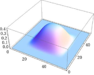
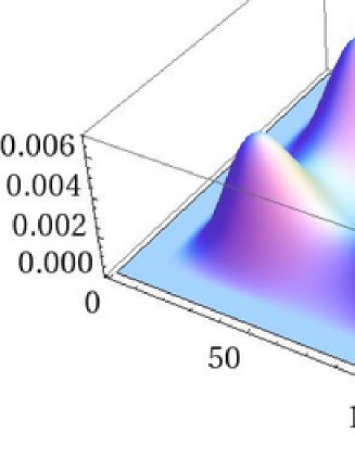
(a)                                                     (b)

Figure 2: Typical electronic charge densities showing the feature of incipient Wigner localization for four electron quantum dot. (a) The charge density in low $r_{s}$ regime while (b) that in low density regime (high $r_{s}$). The imergence of four peaks in (b) is the indicative of incipient Wigner localization.

It is of equal interest to analyze the effect of impurity to on the charge densities seen above. Figure 3 shows the evolution of charge density of same quantum dot in presence of the impurity. Impurity being attractive in nature produces the peak in the charge density. It should be pointed out that as the size of the dot is increased the charge in the dot spreads over larger area while the charge inside the impurity remain confined within the same region giving rise to relatively large peak seen in figure 3 (b).

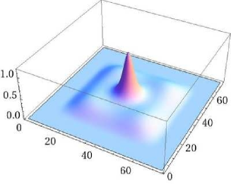
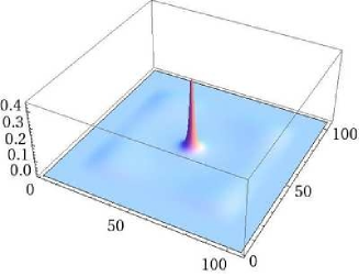
(a)                                                     (b)

Figure 3: Evolution of the charge density of the dot as a function of dot size in presence of an attractive impurity. (a) Impurity being attractive in nature gives rise to peak seen at the center. (b) In low density regime the available area for electrons being sufficiently large the electron spread away and only electron trapped inside the impurity give relatively large peak. Four small peaks are also developed in the four corners.

The impurity is tuned in such a way that traps an electron inside it, thus giving rise to localized magnetic moment. In many quantum dots this localization is associated with peculiar anti-ferromagnetic-like coupling with firm unit magnetic moment at the center and four peaks at the corners for opposite spins. Our DFT analysis indicates that the presence of impurity may change the ground state of quantum dot from magnetic to nonmagnetic and vice versa. We also observe the oscillations in the charge density along the walls of the dot as function of number of electrons.

4.2 Atomic clusters

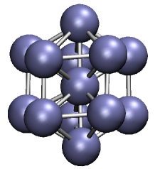
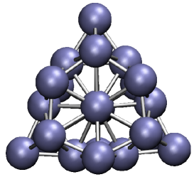
(a)                                            (b)

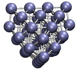
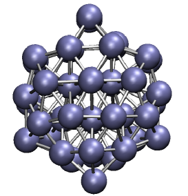
(c)                                            (d)

Figure 4: Evolution of the gallium cluster as we go on increasing the constituent atoms. The geometries are for (a) Ga₁₃, (b) Ga₂₄, (c) Ga₃₆ and (d) Ga₄₇.

The main objective here is to obtains several equilibrium geometries of gallium clusters in the size range of $n=$ 13-55 [3]. Authors examined the evolutionary trends as the clusters grow. Figure 4 shows few representative equilibrium geometries obtained, which highlight the evolution process of the shapes of clusters with growth in their size.

As can be seen from the figure, the geometries represent several ordered and disordered structures. It was seen that addition of few atoms can drastically change the order of the system. Similar observations on larger scale were also reported by Ghazi et al [11]. Gallium clusters show the tendency of forming planer (or slab-like) structures. Further it was seen that most of the bonds in the cluster are of sp² type, which is unlike aluminium clusters which imply that the Gallium clusters do not fit into the simple jellium-like model.

To examine the stability of the cluster it is instructive to analyze the binding energy per atom of the cluster. Binding energy per atom is the amount of energy required to remove an atom completely from the cluster. Thus, higher the binding energy stronger the cluster. Figure 5 shows the binding energy per atom for the clusters ranging from 13 to 48. It is clear from the figure that the clusters with increasing number of atoms are more stable. The binding energy per atom tend to saturate as the number of atoms increases.

Figure 5: Binding energy per atom for gallium clusters ranging from $n=13$ to 48. Increasing binding energy per atom indicates that the larger clusters are more stable than the smaller ones.

Based on the conclusion of both the works [3, 11], it is clear that the growth shows an order-disorder-order pattern. In fact we found that even in the disordered cluster there are hidden interlinked ordered structures. Authors observed that between two ordered structures the growth proceeds via disordered clusters having multicentered icosahedral local order. The transition from disordered to ordered structure is rather sharp and occurs merely on changing the number of atoms by two or three. It was also found that the geometries strongly influence the melting temperature of the given cluster.

4.3 Management of the jobs

A typical problem faced when we handle such large scale problems is the implementation and the management of the jobs involved. All together we have several thousands of jobs in both the problems and it is extremely desirable to have a tool which can assist in handling such enormous number of jobs. Understandably submitting, monitoring and retrieving each job manually is a tedious and time consuming procedure and any web-based application may turn out to be inefficient. We seek the simple solution in the form of shell scripts. It turned out that the scripts are easy to use, highly customizable and equally efficient tool for implementing and managing the jobs.

5 Summery

Thus to summarize, we have successfully implemented the Grids for the large scale problem in the condensed matter physics. We have demonstrated that the commonly used Density Functional Theory based calculations can be performed on Grids. The nature of the problems involve large number of independent jobs to be carried out where the Grid turned out to be most useful. For the management of the jobs we mainly relied on standard Shell Script instead of any web-based porting tool.

References

- [1] B. S. Pujari, K. Joshi, D. G. Kanhere, and S. A. Blundell. Phys. Rev. B, 76:085340, 2007.
- [2] B. S. Pujari, K. Joshi, D. G. Kanhere, and S. A. Blundell. Phys. Rev. B, 78:125411, 2008.
- [3] V. V. Kaware, M. Manerikar, K. Joshi, and D. G. Kanhere. To be published.
- [4] M. Reed. Sci. Ame., 268:118, 1993.
- [5] R. C. Ashoori. Nature, 379:413, 1996.
- [6] S. M. Reimann and M. Manninen. Rev. Mod. Phys., 74:1283, 2000.
- [7] A. Ghosal, A. D. Güçlü, C. J. Umrigar, D. Ullmo, and H. U. Baranger. Phys. Rev. B, 69:153101, 2004.
- [8] Ideh Heidari, Sourav Pal, B. S. Pujari, and D. G. Kanhere. J. Chem. Phys., 127:114708, 2007.
- [9] P. Gori-Giorgi, C. Attaccalite, and S. Moroni G. B. Bachelet. Int. J. Q. Chem., 91:126–130, 2003.
- [10] B. Tanater and D. M. Ceperley. Phys. Rev. B, 39:5005, 1989.
- [11] S. M. Ghazi, S. Zorriasatein, and D. G. Kanhere. J. Phys. Chem. A, 113:2659, 2009.
- [12] F. Baletto and R. Ferrando. Rev. Mod. Phys., 77:371, 2005.
- [13] J. P. Perdew and Y. Wang. Phys. Rev. B, 45:13244, 1992.
- [14] E. P. Wigner. Phys. Rev., 46:1002, 1934.
- [15] S. Akbar and I. Lee. Phys. Rev. B, 67:235307, 2003.