Complex Structure in Class 0 Protostellar Envelopes

Abstract

We use archived IRAC images from the Spitzer Space Telescope to show that many Class 0 protostars exhibit complex, irregular, and non-axisymmetric structure within their dusty envelopes. Our 8 $\mu$m extinction maps probe some of the densest regions in these protostellar envelopes. Many of the systems are observed to have highly irregular and non-axisymmetric morphologies on scales $\gtrsim$ 1000 AU, with a quarter of the sample exhibiting filamentary or flattened dense structures. Complex envelope structure is observed in regions spatially distinct from outflow cavities, and the densest structures often show no systematic alignment perpendicular to the cavities. These results indicate that mass ejection is not responsible for much of the irregular morphologies we detect; rather, we suggest that the observed envelope complexity is mostly the result of collapse from protostellar cores with initially non-equilibrium structures. The striking non-axisymmetry in many envelopes could provide favorable conditions for the formation of binary systems. We also note that protostars in the sample appear to be formed preferentially near the edges of clouds or bends in filaments, suggesting formation by gravitational focusing.

1 Introduction

Sphericity and axisymmetry have been standard assumptions on which our theoretical understanding of star formation has rested for some time. One of the early models of protostellar collapse by Shu (1977) was based on the singular isothermal sphere developed and extended to include rotation by Terebey et al. (1984, TSC). Further modifications have been introduced over time, including models with flattened envelopes or ‘pseudo-disks’ as in Galli & Shu (1993) and Hartmann et al. (1996) while still assuming axisymmetry. Spherical/axisymmetric envelope models have been used extensively to calculate spectral energy distributions (SEDs) of embedded protostars or disks (e.g. Kenyon et al., 1993; Whitney & Hartmann, 1993; Whitney et al., 2003). In particular, the TSC envelope model has been highly successful in modeling the SEDs of Class 0 and Class I protostars; by including outflow cavities, such models are also able to reproduce near and mid-infrared scattered light images (e.g. Adams et al., 1987; Furlan et al., 2008; Kenyon et al., 1993; Stark et al., 2006; Tobin et al., 2007, 2008). However, it is not clear whether or not envelopes around protostars are accurately described by symmetric models.

Recently, observations with the Spitzer Space Telescope have given a high-resolution view of envelope structure around two Class 0 protostars in extinction at 8$\mu$m against Galactic background emission, L1157 appears flattened and L1527 has an asymmetric distribution of material (Looney et al., 2007; Tobin et al., 2008). This method enables us to observe the structure of collapsing protostellar envelopes on scales from $\sim$1000AU to 0.1 pc for the first time with a mass-weighted tracer. In contrast, single-dish studies of envelopes using dust emission in the sub/millimeter regime generally have lower spatial resolution. The continuum emission depends upon temperature as well as mass, while molecular tracers are affected by complex chemistry. Interferometry can provide higher resolution of both continuum and molecular tracers, but large scale structure is resolved out, in contrast to the 8 $\mu$m extinction maps.

In this paper, we analyze archival IRAC images of 22 Class 0 protostars whose dusty envelopes can be detected in extinction at 8$\mu$m. Most of the envelopes in our sample are found to be irregular and non-axisymmetric. We demonstrate that the extinction we observe is indeed due to the circumstellar envelope and not background fluctuations by comparing near-IR extinction measurements with those at 8$\mu$m. Near-infrared imaging of lower-extinction regions is used to correct for foreground emission and/or instrumental effects. We also derive quantitative measures of the envelope asymmetries using projected moment of inertia ratios. Our results indicate that infalling envelopes are frequently complex and non-axisymmetric, which might be the result of gravitational collapse from complex initial cloud morphologies. We also suggest that protostars exhibit a preference to form near the edges of clouds or bends in filaments, which could be due to the effects of gravitational focusing.

2 Observations and Data Reduction

The primary dataset used in this study is comprised of archived Spitzer Space Telescope 8$\mu$m images taken with the IRAC instrument. We have also taken near-IR (H & Ks-band) images of the protostars and surrounding regions with a rich stellar background as an additional constraint on column density using near-IR extinction mapping via the near-infrared color excess (NICE) method (Lada et al., 1994).

2.1 Spitzer IRAC Observations

Motivated by prior detections of envelopes in extinction, we downloaded the pipeline-reduced data for cataloged Class 0 protostars (e.g. Froebrich, 2005; Seale & Looney, 2008) as well as the c2d (Evans et al., 2003) observations of dense cores and molecular clouds to determine if a protostar has an 8$\mu$m extinction envelope associated with it. Of the cataloged protostars, we have clearly detected 22 envelopes in extinction within the nearby star forming clouds (Taurus, Perseus, Cepheus, Chameleon, Orion). We were not able to obtain meaningful results for sources in which the background emission is too faint to reliably derive $8\mu$m extinction, or in cases where the protostar is too bright, thus swamping its envelope structure with emission on the wings of the point-spread function (PSF), or in very crowded regions with many protostars, outflows, and extended foreground (PAH) emission. Pre-stellar/starless cores (e.g., Stutz et al. (2009) and Bacmann et al. (2000)) are not considered in this study.

For each source with identified extinction, we downloaded the basic calibrated data (BCDs) and mosaicked the individual frames using MOPEX after running the Spitzer IRAC artifact mitigation tool written by S. Carey. Because the IRAC data use sky darks rather than true darks, all dark frames contain some level of zodiacal light emission that is subtracted from the BCDs. For our purposes, it is necessary to eliminate the zodiacal light from our images. Thus, during the artifact mitigation process we subtracted the difference between the zodiacal background of the target and the sky dark zodiacal background as written in the BCD headers which are determined from a zodiacal light model (Meadows et al., 2004).

We list the selected sources, observations dates, integration times, and AOR keys in Table 1. The sources in which the data were originally observed by the authors are also identified with the program number. Also, some objects had multiple epochs of observation. In these cases, the datasets were combined if the data were taken close enough in time such that the difference between estimated zodiacal emission was negligible. If the observations were taken more than a few days apart, we used the set of observations with the longest integration time.

2.2 Near-IR Observations

To complement our Spitzer 8$\mu$m data, we observed selected protostars from our sample in H and Ks-bands for the purpose of measuring extinction toward background stars viewed through the envelope. We have identified the protostars for which near-IR data were taken in Table 1. Data for L1152, L1157, L1165, L723, and L483 were taken at the MDM Observatory on Kitt Peak using the near-IR instrument TIFKAM on the the 2.4m Hiltner telescope during photometric conditions between 29 May 2009 and 4 June 2009. TIFKAM provides several imaging modes, we used the F/5 camera mode which provides a $\sim$5^′ field-of-view (FOV) over the 1024² array. We observed the targets in a 5-point box dither pattern with 30^′′ steps, taking 5x30 second coadded images at each point in H and Ks-bands. Total integration times were generally 50 minutes in Ks-band and 40 minutes in H-band, these were varied depending on seeing and sky-background. We were not concerned with preserving extended emission from the protostars, therefore we median combined the images of a single dither pattern to create a sky image for subtraction. The data were reduced using the UPSQIID package in IRAF.

The observations of BHR71, IRAS 09449-5052, and HH108 were taken with the ISPI camera (van der Bliek et al., 2004) at CTIO using the 4m Blanco Telescope during photometric conditions on 11 June 2009. The ISPI camera features a 10.5^′ FOV on a 2048² array. We observed the protostars using a 10-point box dither pattern with 60^′′ steps with 3x20 second coadded images in Ks-bands and generally 2x30 second coadded images in H-band. The total integration time for BHR71 was 30 minutes in each band, and 20 minutes for IRAS 09449-5052. Again, we median-combined the on-source frames to create the sky image; however, due to the larger field and steps in the dither pattern extended emission is preserved in these data. We used standard IRAF tasks for flat-fielding and sky subtraction. We could not simply combine the data using an alignment star due to optical distortion. To correct for this, we fit the world-coordinate system (WCS) to each flat-fielded, sky-subtracted frame using wcstools (Mink, 1999) and the 2MASS catalog. Then we used the IRAF task CCMAP to fit a 4th order polynomial to the coordinate system. A difficulty encountered was the lack of 2MASS stars in the center of the images since our targets are protostars with highly opaque envelopes. In addition, the 2MASS catalog tends to have some false source identifications associated with diffuse scattered light in the outflow cavity of protostars. Thus, since not all polynomial fits were acceptable, we applied the best fitting solution to all images. We then used the stand-alone program SWARP (Bertin et al., 2002) to combine the individual frames while accounting for the distortion.

Lastly, we conducted additional observations of BHR71 with the PANIC camera on the 6.5m Magellan (Baade) telescopes. The data were taken during photometric conditions on 17 and 18 January 2009. The PANIC instrument has only a $\sim$2^′ FOV, thus we took 3 fields of BHR71, one centered on the protostar, one 2^′ east and 45^′′ south, and a last field 2^′ west and 45^′′ north. The data were taken in a 9-point dither pattern with 2x20 second images taken at each position (coadds are not supported with PANIC). The total integration time for each field was 12 minutes in H and Ks-bands. The seeing during these observations was $\sim 0.4^{\prime\prime}$; thus, these images detect fainter stars despite shorter integration times than to the ISPI observations. Separate offset sky observations were taken for the central field, the east and west fields were median combined to create the sky image. The data were reduced using the UPSQIID package in IRAF.

For all the above datasets, photometry of stars in the images was measured using the DAOPHOT package in IRAF. We used DAOPHOT to identify point-sources, create a model PSF from each combined image, and measure instrumental magnitudes using PSF photometry. The magnitude zeropoints were determined by matching the catalog from DAOPHOT to the 2MASS catalog and fitting a Gaussian to a histogram of zeropoint measurements. The H and Ks-band catalogs were then matched using a custom IDL program which iteratively finds corresponding star in each catalog and computes the $H-Ks$ color. Only sources with detections at H and Ks-bands were included in the final catalog.

3 Results

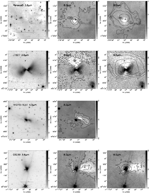
Figure 2: Same as Figure 1 except one-sided envelopes are shown. The 8.0 $\mu$m optical depth contours correspond to the following values of $\tau_{8\mu m}$ for Perseus 5: 0.75, 1.22, 2.0; L1527: 0.1 0.375, 1.4; HH270 VLA1: 0.34, 0.6, 2.4; CB230: 0.3, 0.67, 1.5.

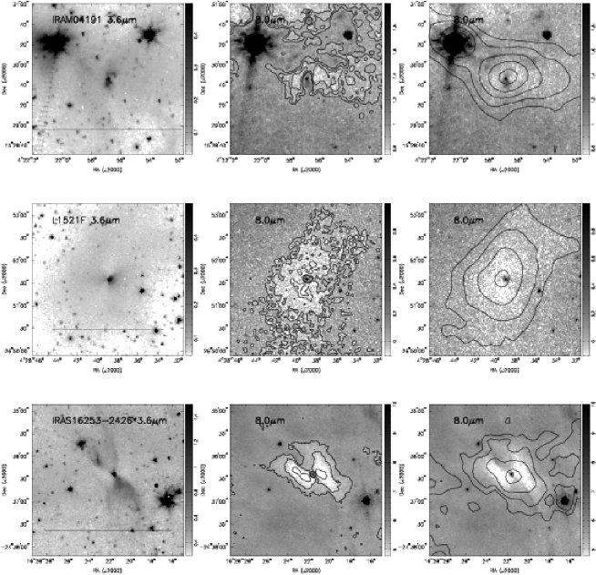
Figure 3: Same as Figure 1 except spheroidal envelopes are shown. The 8.0 $\mu$m optical depth contours correspond to the following values of $\tau_{8\mu m}$ for IRAM 04191: 0.4, 0.57, 0.8; L1521F: 0.6, 0.85, 1.2; IRAS 16253-2429: 0.3, 0.53, 0.95.

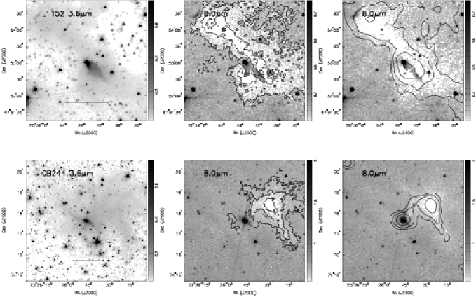
Figure 4: Same as Figure 1 except binary envelopes are shown. The 8.0 $\mu$m optical depth contours correspond to the following values of $\tau_{8\mu m}$ for CB244: 0.3, 0.72, 1.75; L1152: 0.45, 0.91, 1.85.

In Figures 1-5, we display the 22 systems for which we have detected an envelope in extinction. The 3.6$\mu$m image is shown in the left panels, the 8.0$\mu$m image with optical depth contours (see §4) from 8$\mu$m data in the middle panel, the 8.0$\mu$m image with SCUBA 850$\mu$m contours overlaid in the right panel. In the case of HH108, (Figure 1) there were no IRAC data, so we plot the Ks-band image, MIPS 24$\mu$m image and optical depth contours and the Ks-band image with SCUBA 850$\mu$m contours overlaid. The 3.6$\mu$m/Ks-band image for each source shows the scattered light cavity and, for some of the data with very deep integrations, the envelopes are outlined by diffuse scattered light. The 8.0$\mu$m images and optical depth contours show the envelope structure in extinction, and the overlaid SCUBA data from Di Francesco et al. (2008) show how the thermal envelope emission correlates with the 8.0$\mu$m extinction.

The most striking feature of the 8$\mu$m extinction maps is the irregularity of envelopes in the sample. Most envelopes show high degrees of non-axisymmetry; in most cases, spheroids would not provide an adequate representation of the structure. Some of the most extreme examples have most extincting material mostly on one side of the protostar (e.g. CB230, HH270 VLA1) or the densest structures are curved near the protostar (e.g. BHR71, L723). The structures seen in extinction at 8$\mu$m do not seem to be greatly influenced by the outflow. The 3.6$\mu$m images show that the outflow cavities of these sources are generally quite narrow, with a relatively small evacuated region; the dense material detected in extinction is often far from the outflow cavities and thus seems unlikely to be produced by outflow effects (see §6.1 for further discussion).

For convenience, we categorize the systems into 5 groups according to their morphology, though some systems have characteristics of multiple groups. Figure 1 shows the envelopes that have a highly filamentary or flattened morphology; Figure 2 shows envelopes that have most material (in projection) on one side of the protostar; Figure 3 shows the protostars whose envelopes are more or less spheroidal in projection; Figure 4 shows the protostars which appear to be binary (i.e., one protostar is present and about 0.1 pc away there is an extinction peak probably corresponding to a starless core). Lastly, Figure 5 shows envelopes that do not strictly fall within the above categories, and are simply classified as irregular.

This dense complex structure is less apparent in the SCUBA maps primarily because it has a resolution of $\sim$ 12^′′ at 850$\mu$m while IRAC has a diffraction limited resolution of $\sim$2^′′. SCUBA also has limited sensitivity to extended structure due to the observation method; thus IRAC can better detect non-axisymmetries on smaller and larger scales than seen in SCUBA maps. In addition, the strongest emission from most envelopes appears to be axisymmetric because the protostar is warming the envelope (Chiang et al., 2008, 2009); the extinction maps are not affected by the envelope temperature distribution.

4 Optical Depth Maps

Though the morphology of extincting material is clear from direct inspection of the images, it is desirable to convert the 8 $\mu$m intensities to optical depth maps to make quantitative measurements. Initially we assumed that the observed intensities can be interpreted as pure extinction with no source emission, i.e.

$$\frac{I_{obs}}{I_{bg}}=e^{-\tau}$$ (1)

where $I_{obs}$ is the observed intensity per pixel and $I_{bg}$ is the measured background intensity, both corrected for the estimated zodiacal light intensity as discussed in §2.1. However, our attempts to model the filamentary structure in L1157 (§5.2) and the very low column densities measured led us to conclude that our maps contain more foreground emission and/or zero-point correction than we originally thought. This may not be surprising, as measurements of the zodiacal light intensity during the Spitzer First Look Survey were 36% higher than predicted by the model (Meadows et al., 2004). Either there is residual zodiacal light not accounted for by the model, or there is foreground dust emission, scattered light within the detector material (Reach et al., 2005), or some combination of these factors. Unfortunately, because IRAC operates without a shutter, it is impossible to determine the true level of diffuse emission.

Thus, in our initial analysis we were calculating

$$\frac{I_{obs}+I_{fg}}{I_{bg}+I_{fg}}=e^{-\tau}$$ (2)

which will yield an erroneously low value of $\tau$. This is because as $I_{fg}$ increases, the ratio of $I_{obs}^{\prime}$/$I_{bg}^{\prime}$ increases, causing the measured optical depth to decrease.

We therefore obtained the ground-based near-infrared imaging data to develop an independent estimate of the extinction in lower-column density areas, and thus made a better estimate of the foreground contribution. The Ks-band images of BHR71 and L483 with optical depth contours overlaid in Figure 6 show that many background stars can be detected through to dense envelope. The details of the foreground correction are discussed in the Appendix.

With the estimated foreground contribution was subtracted, we were able to calculate a more accurate optical depth map following Equation 1. We now must calculate the background emission in the image; fortunately in most images the background is relatively uniform. We estimated the background emission by fitting a Gaussian to a pixel histogram constructed from an area in the image not affected by the extinction of the envelope. For the sources IRAS 05295+1247, HH211, and L1165, the background has clear gradients. To account for this, we constructed a background model by performing a two-pass median filter of the entire image with a convolving beam 90^′′ (IRAS 05295+1247) and 144^′′ (L1165, HH211) in size; this method is similar to that of Simon et al. (2006); Ragan et al. (2009); Butler & Tan (2008). We used the first pass to identify stars in our background measurement field, then rejected those pixels in the second pass. The median background computed from the first and second passes are generally within a few percent of each other. The large convolving beam ensures that we filter out the envelope from the background model.

We then divided each pixel by the background value, or, in the case of IRAS 05295+1247/L1165, we divided the intensity map by the background model. Then taking the natural logarithm of each pixel intensity yielded the optical depth map. In the case of HH108, we constructed an optical depth map from the MIPS 24$\mu$m image because there are no IRAC data for this object.

We give the values of $I_{fg}$, $I_{bg}^{\prime}$ (see Appendix), $\tau_{max}$, and $\sigma\tau$ for each source in Table 2. In all cases, $I_{fg}$ is comparable to measured intensity at the darkest spot in the uncorrected 8$\mu$m image. Thus, we can infer than the darkest part of an envelope is completely opaque. To set an upper limit on the optical depth in these areas, we use the pixel value in the uncertainty image as $I_{obs}$ and compute the optical depth; this is the maximum optical depth ($\tau_{max}$)in an image. To correct our images without near-IR data, we use the result that in the most opaque areas of the images $I_{fg}$ is the observed intensity and take this value as an estimate of the foreground contribution.

5 Quantitative Results

5.1 Non-Axisymmetric Structure

To quantify the evident envelope asymmetry of many sources, we calculate projected moment of inertia ratios using $\tau$ as a surrogate for mass. We calculate the ratios by computing

$$\frac{I_{\perp}}{I_{\parallel}}=\frac{\sum_{i}\tau_{i}(x_{i}-x_{\circ})^{2}}{\sum_{j}\tau_{j}(y_{j}-y_{\circ})^{2}}$$ (3)

where $x_{\circ}$ and $y_{\circ}$ are the coordinates of the protostar and $I_{\perp}$ is the moment of inertia of material distributed perpendicular the outflow along the abscissa and $I_{\parallel}$ is for material located parallel to the outflow axis along the ordinate axis. The subscripts $i$ and $j$ denote the independent points where the optical depth is measured. We rotate the optical depth images such that the outflow is along the ordinate axis of the image to simplify interpretation. We also calculate the moment of inertia ratios for $I_{\perp}$ left and right of the protostar ($I_{\perp,l}$/$I_{\perp,r}$) and the same for $I_{\parallel}$ ($I_{\parallel,l}$/$I_{\parallel,r}$). We measure the ratios out to a radius of 0.05 pc for most protostars at the adopted distance in Table 1 and we set an inner radius of 0.01 pc.The outer radius is restricted so the moments of inertia are sensitive to the densest structures closest to the protostar and not influenced by extended diffuse material. Also, areas where emission is present are masked by requiring that the optical depths be positive.

Each ratio quantifies a different aspect of the distribution of material around the protostar. $I_{\perp}$/$I_{\parallel}$ describes how much material is located along the outflow axis versus perpendicular to it, a ratio greater than 1 would correspond to more material away from the protostar, perpendicular to the outflow. A ratio less than 1 corresponds to having more material close to the outflow axis, extended in the direction of the outflow. $I_{\perp,l}$/$I_{\perp,r}$ describes the asymmetry about the outflow axis by comparing the measurements on the right and left sides of the protostar and $I_{\parallel,l}$/$I_{\parallel,r}$ describes the asymmetry about the outflow but in the vertical direction. Taken together these ratios describe the distribution of material around the protostar, convenient for comparison to theoretical models.

The projected moment of inertia ratios for the envelopes are given in Table 3. There are more envelopes that are extended perpendicular to the outflow than along it (most $I_{\perp}$/$I_{\parallel}$ ratios are $>1$). Many objects exhibit large ratios and they can be described as highly flattened/elongated. HH270 VLA1 and L1152 seem to be the only examples of envelopes strongly extended in the direction of their outflows in our sample. However, both L673-SMM2 and Serp-MMS3 have components of their envelopes oriented parallel and perpendicular to their outflows. This yields a $I_{\perp}$/$I_{\parallel}$ ratio $\sim$1 but in the other ratios, non-axisymmetry is evident.

The most symmetric envelope is IRAS 16253-2429, as shown by its moment of inertia ratios all being near 1. The two most non-axisymmetric envelopes appear to be HH270 VLA1 and CB230. HH270 VLA1 has most of its material located southwest of the protostar and CB230 has most of its material located to the west and in a moderately-flattened configuration.

5.2 Flattened Structure

There are six sources that have remarkably flat structure compared to the rest of the sample, shown in Figure 1: L1157, L723, HH108, Serp-MMS3, L673-SMM2, and BHR71. With respect their molecular outflows, L1157 and BHR71 are viewed nearly edge-on; the primary protostar in HH108 seems to be edge-on as well. Serp-MMS3 and L673-SMM2 are not well studied; however, 3.6$\mu$m image of Serp-MMS3 indicates that it is at least inclined by 60^∘ or more and L673-SMM2 harbors several protostars and their inclinations are not known. The orientation of L723 is uncertain as there are two embedded sources driving outflows and due to the complexity of the data we omit this object from our analysis.

For these sources, we ask the question: are these envelopes flattened sheets/pseudo-disks (Hartmann et al., 1994, 1996; Galli & Shu, 1993) or filaments? To attempt to answer this question, we compare the observed vertical structure of the flattened envelopes to analytic prescriptions for isothermal hydrostatic filaments and sheets.

The scale height of an isothermal filament in hydrostatic equilibrium is

$$H_{f}=\frac{c_{s}^{2}}{2G\Sigma_{0,f}}$$ (4)

where $c_{s}$ is the isothermal sound speed, we assumed T=10K, and $\Sigma_{0,f}$ is the peak surface density measured at the center of the filament (Hartmann, 2009). When parametrized in terms of 8$\mu$m optical depth and assuming $\kappa_{8}$ = 10.96 cm²g^-1,

$$H_{f}=\left(\frac{0.96}{\tau_{0,f}}\right)\left(\frac{T}{10K}\right)^{-1}\times 0.01pc.$$ (5)

Thus, a 10 K filament with a scale height of 0.01 pc will have $\tau$ $\sim$1 at 8$\mu$m.

Similarly, the scale height of an isothermal infinite sheet is given by

$$H_{s}=\frac{c_{s}^{2}}{\pi G\Sigma_{0,s}}.$$ (6)

In this case, $\Sigma_{0,s}$ is not the surface density measured at the center of the sheet viewed edge-on but it is the surface density through the z-direction of the sheet. Thus, we must make an assumption about depth of the sheet into the line of sight. Making the same assumption about temperature as the filament case, we can write the scale height of a sheet as

$$H_{s}\sim\frac{1.2}{\tau_{0,f}}\left(\frac{d}{t}\right)(0.01pc)$$ (7)

where $d$ is the line-of-sight depth through the sheet and $t$ is the thickness of the sheet in the plane of the sky. Together, $d$ and $t$ specify the aspect ratio of the sheet; $d$ is assumed to be 0.1 pc (the diameter of most envelopes in the sample) and $t$ is taken to be the FWHM of the Gaussian fit to the vertical structure described in the next paragraph. For an aspect ratio of 10, the peak optical depth would have to be $\sim$12 in order to have a scale height of 0.01 pc.

We analyzed the structure by averaging the extinction map along the extended dimension in three pixel bins, and then fitting a Gaussian to the perpendicular structure in each bin. The peak of the Gaussian fit is taken to be the central optical depth. Then, in Figure 7 we compare the observed vertical structure to the expected vertical structure for a filament and sheet as a function of distance from the protostar, converting from the Gaussian $\sigma$ parameter to $H$ (for instance, we find that $\sigma\sim 1.5H$ for a filament).

For the case of L1157, the 10 K hydrostatic filament appears to be in reasonable agreement with the observed extinction, while the sheet scale height is about a factor of 3 than observed. If we do not correct the 8$\mu$m extinction for foreground emission, the predicted filament scale heights were a factor of 5 too large. As it is hard to imagine anything thinner than a pressure supported filament, this result is further verification of the need for correcting the 8$\mu$m extinctions for foreground emission.

The envelope around Serp-MMS3 is also fit well by a filament over $\sim$0.1pc. We only fit the northeast part of the filament for this source because the data of the southwest portion of the envelope is quite complicated. In L673-SMM2, we attempted to fit both the north and south portions of the filament, avoiding the region near the protostars. The filament model does not fit as well as L1157 or Serp-MMS3; the observed scale heights are always less than those predicted for a filament. We suspect that this discrepancy is due to the densest part of the filament being unresolved, underestimating the peak column density.

Neither sheet nor filament models yielded good fits to BHR71 which has a more complicated envelope structure than L1157 and a larger optically thick region. The predicted scale height for a filament tends to be about 2.5 times smaller than observed; thus a sheet seems to be more consistent with the observed data. Alternatively, the dense structure may not be in hydrostatic equilibrium.

5.3 Mass Estimates

With our optical depth maps at 8.0 $\mu$m, we have the opportunity to estimate envelope masses independently of the temperature and chemical effects. Our results do depend on the assumed opacity, but recent extinction law studies using Spitzer have yielded better constraints on the opacity at 8$\mu$m. However, we cannot trace column density in regions where the envelope is optically-thick.

To derive a column density from the optical depths, we assume the dust plus gas opacity $\kappa_{8\mu m}=10.96$ cm² g^-1 (Butler & Tan, 2008) which corresponds to the Weingartner & Draine (2001) $R_{V}$ = 5.5 Case B dust model which found to agree reasonably well with the extinction laws derived at IRAC wavelengths (Román-Zúñiga et al., 2007; McClure, 2009). This opacity is calculated by convolving the IRAC filter response with the expected background spectrum shape, and opacity curve.

To calculate the mass of a particular envelope, we simply sum all the pixels with $\tau$ greater than $\sigma\tau$ within 0.15, 0.1, and 0.05 pc radii around the envelope and assume the relation

$$M_{env}=d\Omega\times D^{2}\times(1.496\times 10^{13}\frac{cm}{AU})^{2}\times\sum_{i}^{N}\frac{\tau_{i}}{\kappa}$$ (8)

where $d\Omega$ is the pixel solid angle, (1.2^′′)², and $D$ is the distance in parsecs.

The masses determined using this method are probably lower limits at best because most envelopes become completely opaque in the densest areas. Moreover, the uncertainty in optical depth increases as optical depth increases. We are also probably not sensitive to some mass on large scales due to signal-to-noise limitations and on small scales emission is present which prevents measurement of optical depth.

The measured envelope masses are given in Table 2 along with the measurements from ammonia and submillimeter studies. The 0.05 pc radius is probably most comparable to the mass measurements from the other methods. This is because most ammonia cores are generally about 0.1-0.15 pc in diameter and submillimeter fluxes are generally measured in apertures with diameters of 80-120^′′ which correspond 0.1 - 0.15 pc in diameter for an assumed distance of 300 pc. The masses we measure are comparable with the other methods at smaller radii.

A specific trend that we see is that some protostars are surrounded by significant mass at large and small radii. All the protostars in the sample are have nearly 1 M_☉ of material within 0.05 pc; there is possibly even more mass within 0.05 pc since we do no probe the regions where the protostar is emitting and the material could be optically thick. Even the very low-luminosity protostars (e.g. IRAM 04191, L1521F, Perseus 5) are surrounded by many solar masses of material. For reference we also list the bolometric luminosities for the observed sources in Table 2, there is no obvious correlation between luminosity and envelope mass.

6 Discussion

The observations of dense, non-axisymmetric structures in Class 0 envelopes have significant implications for our understanding of the star formation process. The dense structures that we observe either result from the initial conditions of their formation or they have been induced on an otherwise axisymmetric envelope during the collapse process. We will discuss why these dense structures are not likely induced by outflows, the most obvious perturber, and then discuss how non-axisymmetric infall could affect subsequent evolution of the system. We also discuss how the envelope structures may give clues to the initial conditions of their formation and what relationship the larger scale cloud structure around the protostar may have on its formation.

6.1 Outflow-induced structure

Outflows carve cavities in protostellar envelopes and necessarily affect the structure of the protostellar environment at some level. However, it is highly unlikely that outflows are responsible for much of the complex envelope morphology we observe. While a few objects such as L1527 exhibit relatively wide molecular outflows and outflow cavities (e.g., Jørgensen et al. (2007)), most of our outflow cavities (as seen most clearly in scattered light at $3.6\mu$m, but also detectable in the 8.0 $\mu$m images) are relatively narrow and well-collimated, in agreement with molecular observations (e.g. Arce & Sargent, 2006; Jørgensen et al., 2007); this makes it difficult to imagine that the outflow is strongly affecting most of the envelope. Moreover, if the observed dense, asymmetric envelope structures were the result of outflow sculpting, we would expect close spatial association of these structures with the outflow cavities; in contrast, the cavities in most objects are spatially distinct from the dense structures, sometimes by quite large distances, and with no systematic alignment perpendicular to the cavities.

HH270 and IRAS 16253 are exceptions to this general rule, with strong concentrations of extinction along cavity walls; however, both these systems are strongly asymmetric perpendicular to the outflow cavities, which indicates that the density structures are mostly the result of existing inhomogeneities in the ambient medium. Similarly, it has been suggested that the outflow in L483 is strongly affecting molecular material based on observations of N₂H⁺ emission ((Jørgensen, 2004)); however, the strong density enhancement on one pole of the outflow relative to the other is difficult to understand as purely a result of mass loss, given the general bipolar symmetry of most systems.

To summarize, the outflows do not appear to have significantly affected the current envelope morphologies in most cases. The spatial separation of the outflow cavities and the dense, extincting structures make it less likely that outflows can significantly limit mass accretion onto the central protostar. The common inference that bipolar flows widen with age, dispersing the envelope (e.g. Arce & Sargent, 2006; Seale & Looney, 2008) may result more directly from collapse of dense structures rather than a changing of the outflow angular distribution.

6.2 Dense Non-axisymmetric Structure

The shapes of dense cores have been studied on large scales ($>$0.1 pc) using optical extinction (Ryden, 1996) and molecular line tracers of dense gas (Benson & Myers, 1989; Myers et al., 1991; Caselli et al., 2002). However, optical extinction only traces the surface of dense clouds and most envelopes appear round in the dense molecular tracers because they are generally only spanned by 2.5 beams or less. The low-resolution molecular line studies are slightly more advantageous compared to the optical since they only detect dense material and associated IRAS sources are often located off-center from the line emission peaks indicating non-axisymmetry.

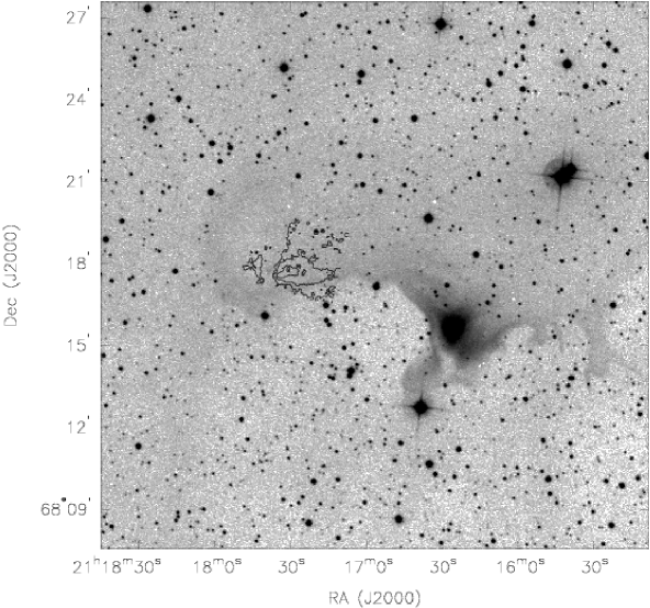
Figure 8: DSS2 red image of CB230 region. The overlaid contours are same optical depth contours as shown in Figure 2 for CB230. The protostar in CB230 has formed on the far eastern side of the cloud while on the western side there is an optical reflection nebula possibly from another recently formed star.

The advantage of 8$\mu$m extinction in studying envelopes compared to other methods is that it provides high resolution, undiminished sensitivity to dense extended structures, and its a tracer that depends only on density. This enables us to trace non-axisymmetric structure from large scales down to 1000 AU scales. Figure 8 exemplifies the details revealed by 8$\mu$ extinction maps; the 8$\mu$m extinction contours of CB230 are overlaid on the optical Digitized Sky Survey image showing the strong asymmetry of dense material while the optical image shows no hint of what is going on at small scales. The necessity of 8$\mu$m extinction to see small scale non-axisymmetric structure holds true for all our sources. The magnitude non-axisymmetry varies significantly between sources; but the important point is that all sources exhibit non-axisymmetry and that sources with “regular” morphology are the exception rather than the rule.

CB230 and the other one-sided envelopes shown in Figure 2 are particularly intriguing. While the outflows may have done some sculpting, the dynamics of the star formation process itself has caused the strong asymmetries perpendicular to the outflow. The curvature of dense structures in BHR71 and L723 as well as the outflow being oriented non-orthogonal to many dense filamentary structures (e.g., L673, HH108, SerpMMS3, L1448 IRS2) may indicate that the angular momentum of a collapsing system may not have a strongly preferred direction set by the large scale cloud structure.

It is important to point out that these non-axisymmetric structures exist down to small scales quite near the protostar and only at about $\sim$1000AU they become obscured by emission from the protostar 8$\mu$m. As shown in Table 2, all the envelopes have a nearly 1 M_☉ or more mass within 0.05 pc. Material we see at $\sim$1000AU potentially has an infall timescale of $\sim$5$\times$10⁴ years and at 10000 AU the infall timescale is about $\sim$5$\times$10⁵ years assuming a 0.96 M_☉ initial core at the start of collapse (§3 (Shu, 1977)). This is consistent with Class 0 protostars having accumulated less than about half their final mass at the present epoch (Myers et al., 1998; Dunham et al., 2010).

6.3 Implications of Non-Axisymmetric Collapse

The envelope asymmetries we see may well result from the initial cloud structure. Stutz et al. (2009) recently surveyed pre-stellar/star-less cores using 8 and 24$\mu$m extinction; their results, and those of Bacmann et al. (2000), showed that even pre-collapse cloud cores already exhibit some non-axisymmetry. Given the initial asymmetries the densest, small-scale regions are likely to become even more anisotropic during gravitational collapse (Lin et al., 1965). We note that gravity is not the only force at work in these clouds; turbulence and magnetic fields may also play roles in forming the envelope morphologies (§6.4).

The smallest scales we observe, $\sim$1000 AU, is where angular momentum will begin to be important as the material falls further in onto the disk. The envelope asymmetries down to small scales imply that infall to the disk will be uneven; therefore, non-axisymmetric infall may play a significant role in disk evolution and the formation of binary systems. Several theoretical investigations (e.g. Burkert & Bodenheimer, 1993; Boss, 1995) showed that collapse of a cloud with just a small azimuthal perturbation can form binary or multiple systems; thus, large non-axisymmetric perturbations should make fragmentation even easier. Fragmentation can even begin before global collapse in a filamentary structure (Bonnell & Bastien, 1993, and references therein). Numerical simulations of disks with infalling envelopes (e.g. Kratter et al., 2009; Walch et al., 2009) informed by the results of this study could reveal a more complete understanding of how non-axisymmetric infall affects the disk and infall process.

Several sources in the sample are known wide binaries (BHR71, CB230) (Bourke, 2001; Launhardt et al., 2001) and close binaries (L1527, L723, IRAS 03282+3035) (Loinard et al., 2002; Girart et al., 1997; Chen et al., 2007). The Spitzer observations indicate that SerpMMS3 may be a binary and that L673-SMM2 is likely a multiple. Other sources in our sample may be close binaries but this property can only be revealed by sub-arcsecond imaging. Looney et al. (2000) showed that many protostars are indeed binary when viewed at high enough resolution at millimeter wavelengths. A recent study of Class 0 protostars at high resolution by Maury et al. (2010) noted that their results taken with Looney et al. (2000) show a lack of close binary systems with 150-550AU separations. This may signify that non-axisymmetric infall throughout the Class 0 phase is important for binary formation later when centrifugal radii extend out to 150-550AU.

6.4 Turbulent formation

The dense, non-axisymmetric structures that we observe around Class 0 protostars are not obviously consistent with quasi-static, slow evolution, which might be expected to produce simpler structures as irregularities have time to become damped. With rotation, one might get a flattened system during collapse, as is well known (Terebey et al., 1984), but one needs non-axisymmetric initial structure to get strong non-axisymmetric structure later on. This raises the question of the role of magnetic fields in controlling cloud dynamics. In some models (e.g. Fiedler & Mouschovias, 1992; Galli & Shu, 1993; Tassis & Mouschovias, 2007; Kunz & Mouschovias, 2009, and references therein), protostellar cores would probably live long enough to adjust to more regular configurations; in addition, collapse would be preferentially along the magnetic field, which would also provide the preferential direction of the rotation axis and therefore for the (presumably magnetocentrifugally accelerated) jets (Basu & Mouschovias, 1994; Shu et al., 1994). The complex structure and frequent misalignment between collapsed structures and outflows pose challenges for such a picture.

In contrast, more recent numerical simulations (e.g. Padoan et al., 2001; Klessen et al., 2000; Ballesteros-Paredes et al., 1999) suggest that cores are the result of turbulent fluctuations which naturally produce more complex structure with less control by magnetic fields amplified by subsequent gravitational contraction and collapse (e.g. Elmegreen, 2000; Klessen et al., 2000; Klessen & Burkert, 2000; Heitsch et al., 2001; Padoan & Nordlund, 2002; Hartmann, 2002; Bate et al., 2003; Mac Low & Klessen, 2004; Heitsch & Hartmann, 2008; Heitsch et al., 2008a, b, see review by Ballesteros-Paredes et al. 2007 (PPV)). Thus, the structure of protostellar envelopes thus provides an indication of which of the two contrasting pictures of core formation, with differing assumed timescales of formation and differing importance of magnetic fields, is more nearly correct.

The timescale argument against ambipolar diffusion can be mitigated since turbulence is known to accelerate ambipolar diffusion Fatuzzo & Adams (2002); Basu et al. (2009). The filamentary envelopes may also enhance ambipolar diffusion as necessary. For example, a cylinder with an aspect ratio of 4:1 (similar to L1157) will have a factor of $\sim$ 10 less volume than a sphere with a diameter equal to the cylinder length. If both have the same infall rate, the filament has a factor of $\sim$ 10 higher density than the sphere. Thus, using

$$\tau_{AD}\sim 5\times 10^{6}\left(\frac{10^{4}cm^{-3}}{n(H_{2})}\right)^{\frac{1}{2}}yr$$ (9)

given in Spitzer (1968), the ambipolar diffusion timescale, $\tau_{AD}$, is reduced by an order of magnitude! With a shorter ambipolar diffusion timescale, the magnetic support of the initial disk could be lower than the levels suggested in Galli et al. (2006), allowing for Keplerian rotation of the resulting circumstellar disk.

The timescale issue aside, it is still difficult to get non-axisymmetric structures from magnetic collapse. Simulations by Basu & Ciolek (2004); Ciolek & Basu (2006) indicated that magnetically sub-critical or critical cores will tend to be round or axisymmetric while the super-critical cores would show higher degrees of non-axisymmetry. Our results are more consistent with fast, super-critical collapse. Further high resolution simulations, such as those by Offner & Krumholz (2009), would help make a better connection between theory and observation.

Alternatively, if a spherical core forms within a turbulent medium, as in Walch et al. (2009), the turbulence within the core itself could give rise to a non-axisymmetric structure. However, two difficulties of this scenario are immediately obvious; first, producing a spherical core in a turbulent environment seems difficult; and second, dense, star forming cores are found to be very quiescent compared to their external medium (Goodman et al., 1998; Pineda et al., 2010). Rather than the core itself being turbulent, anisotropies in the turbulent pressure surrounding a dense core could also give rise to non-axisymmetric structure from an initially symmetric core. One could also envision a scenario where an envelope is impacted by colliding flows causing non-axisymmetries.

6.5 Relationship with Larger Structures

While some systems in our sample seem to be in relative isolation, most are part of large-scale filamentary structure. With the dataset presented, we can examine the spatial relationship of the protostars within their natal material to see if there are trends which influenced by the non-axisymmetries. Here we examine several of the protostars where we can clearly discern the morphology of larger scale material.

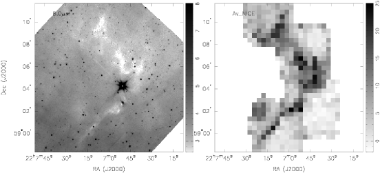
Figure 9: Left: 8$\mu$m image of L1165 region surrounding the protostar(s). The large scale cloud structure shows a highly filamentary structure with a 90^∘ bend near the protostar(s). Right: Extinction map of L1165 region constructed from H and Ks-band imaging taken with TIFKAM, units are in A_V. Despite the lower resolution of the map, the large scale structure is clearly well matched between the two techniques of extinction measurement. The large angular coverage of the dark cloud enabled good calibration of the 8$\mu$m optical depths using the near-IR extinction measurements.

The L1165 dark cloud is comprised of a long filament running from southeast to northwest for $\sim$8^′ (0.6pc) that turns northeast forming a roughly 90^∘ angle and extends $\sim$10^′ (0.75pc). An image of the L1165 region at 8$\mu$m and a near-IR extinction map are shown in Figure 9. Both the protostar (IRS1) and another very bright source about 1.5^′ north (IRS2) have formed near the ‘elbow’ of the filament. IRS2 is likely a young star because the spectral index from 6-13$\mu$m is $\sim$-1 indicating that it is a Class II object. IRS2 is detected at 24$\mu$m (fainter than IRS1) but not at 70$\mu$m. It is intriguing that these two young stars have formed at the ‘kink’ in the filament while there are no apparent protostars elsewhere in the filament. Two other examples of multiple stars forming at filament kinks are L673-SMM2 and Serp-MMS3.

The protostars HH108 IRS1 and HH108 IRS2, (IRAS and MMS respectively in Chini et al. (2001)) have also formed with a filament. HH108 IRS1 is more luminous and IRS2 only appears in emission longward of 24$\mu$m. IRS2 appears as an opaque spot in the 24$\mu$m extinction image in Figure 1. The envelope of IRS1 appears to be a collapsed portion of the larger filament and is located at a bend. On the other hand, the envelope of IRS2 appears round, but slightly extended along the filament.

The protostars CB230 and IRAS 03282+3035 are both located at the edges of dark clouds. We can clearly see the edge of the envelope around IRAS 03282+3035 in diffuse scattered light at 3.6$\mu$m corresponding to the edge of 8$\mu$m extinction (Figure 3). CB230 is an isolated Bok globule, shown in Figure 8. The dark cloud in the optical extends to the west from the protostar $\sim$11^′ (0.95 pc) with highest densities near the protostar at the extreme eastern edge of the cloud. The optical depth map shows the extreme asymmetric distribution of material. In addition, there is an optical star associated with a reflection nebula $\sim$7.25^′ west of the protostar, but it is not detected by IRAS and not observed bySpitzer.

The L1448 dark cloud contains several embedded protostars visible at 8$\mu$m (Tobin et al., 2007). The most isolated protostar is L1448 IRS2, the rest are surrounded by bright emission from outflow knots. IRS1 and IRS2 are located toward the western edge of the cloud IRS3A/B are located on the northeastern corner of the cloud and L1448-mm is located in the southeast corner. There is a filament of material running between IRS2 and IRS3 seen in diffuse scattered light (Figure 1 in Tobin et al. (2007)), 8$\mu$m extinction,and ammonia emission (Anglada et al., 1989). Also, the filament abruptly cuts off $\sim$40^′′ north of IRS2.

Protostars highlighted seem to have a tendency to for to form at the edges of clouds or where there are turns or ’kinks’ in a filamentary structure. This behavior is qualitatively what would be expected if gravitational focusing is important. Put simply, gravitational focusing causes the edges of clouds and where there are discontinuities (bends and kinks) to form stars first by creating gravity focal points. In a filament undergoing global collapse, the ends of that filament will be moving inward the fastest and will encounter slower moving material. This ‘gravitational traffic jam’ creates the gravity focal point. In addition, the filament will also be collapsing in the vertical direction which causes material to flow toward the focal point in from orthogonal directions rather than just the transverse direction. A scenario such as this would cause the ends of the filament to form stars rather than at the center of the filament. Quantitatively, this scenario appears when you modify the spherical (3D) free-fall timescale for a (1D) filamentary geometry. Gravitational focusing is seen in theoretical work by (Burkert & Hartmann, 2004) which simulated a complex object with many thermal Jeans masses. The gravitational focusing causes non-linear collapse near cloud boundaries and other discontinuities (see also Bonnell & Bastien 1993). The results are consistent with a picture in which turbulent fragmentation provides “seeds” which then are amplified by gravity (Heitsch et al., 2008b; Heitsch & Hartmann, 2008).

We note, however, that BHR71 and L483 seem to have formed at the centers of centrally condensed Bok globules, so we cannot claim complete universality for this mechanism. However, the filamentary regions highlighted in the above paragraphs may be representative of star forming environments because the theoretical work shows that turbulent star formation generally gives rise to filaments (e.g. Heitsch et al., 2008b; Heitsch & Hartmann, 2008). Also, the preference of forming stars in clumps at the ends of filaments also appears to apply to young star clusters and loose star-forming associations (e.g. Orion Nebula Cluster, NGC2264, Chameleon, Taurus) (Fűrész et al., 2006, 2008; Tobin et al., 2009; Luhman, 2008; Hartmann, 2002). Thus, gravitational focusing may be at work from the formation of clusters to the formation of individual protostars. Further theoretical work building on that of Burkert & Hartmann (2004) including effects of turbulence and/or magentic fields would enable a better understanding of this idea and determine how much gravity must dominate over other forces present in the cloud.

7 Conclusions

In this paper, we have shown the complex structure of envelopes surrounding Class 0 protostars as viewed in extinction at 8$\mu$m using Spitzer IRAC images. The non-axisymmetries revealed by the IRAC extinction maps were not obvious in submillimeter maps by SCUBA. The 8$\mu$m images were found to be significantly contaminated by foreground emission and we corrected for this using near-IR extinction measurements toward background stars. This method demonstrated that the densest parts of the envelopes observe are completely opaque at the observed signal-to-noise levels. We have characterized the non-axisymmetry of the envelopes in terms of projected moments of inertia ratios. Most envelopes are more extended perpendicular to the outflow, but there are exceptions. Our measurements also yield estimates of the mass surrounding the protostars at small and large scales.

Most envelopes show highly non-axisymmetric structure from $\sim$1000AU to 0.1 pc scales. These asymmetric structures are not caused by outflow-envelope interactions as the outflows are still highly collimated and spatially located away from asymmetric structures and envelopes tend to be more extended perpendicular to the outflow. We suggest that the widening of outflows with age may result more directly from collapse of dense structures rather than a changing of the outflow angular distribution. In the entire sample, we find significant mass present in the envelopes on scales less than 0.05 pc. This supports the idea that Class 0 protostars are in the main phase of mass accretion and the asymmetries of the material down to small scales indicates that material will likely fall onto the disk unevenly possibly enhancing gravitational fragmentation. This could help explain the formation of close binary or multiple systems.

The highly non-axisymmetric envelopes may result directly from the collapse of mildly asymmetric cores found by Bacmann et al. (2000); Stutz et al. (2009) because fast collapse will enhance anisotropies (Lin et al., 1965); turbulence and colliding flows could also play a role in creating asymmetries. The observed structure points to non-axisymmetric and probably non-equilibrium initial conditions. If the magnetic field plays a major role in the collapse process of these envelopes, it is clearly not working to make the infall process more symmetric. Comparison to simulations indicates that super-critical collapse is more consistent with our observations.

Finally, there seems to be a preference of where stars form within larger scale structures. Several systems form protostars at the ends of filaments and at bends or kinks in the more-extended molecular gas, which suggests that the initial shape of a cloud has much to do with where stars form. This is reminiscent of the preference for stars to form in clusters double clusters as we see in local star forming regions such as Orion, NGC2264, and Chameleon.

We thank the anonymous referee for comments enabling us to improve the clarity and impact of this paper significantly. We wish to thank F. Heitsch, Y. Shirley, and A. Stutz for useful discussions and insight. We thank W. Fischer and J. Hernandez for conducting the PANIC observations while J. Tobin was on his honeymoon. We are grateful to the staff of MDM Observatory (R. Barr, J. Negrete, and P. Hartmann) for their support during TIFKAM observations. We thank N. van der Bliek for her support during the ISPI observing run. The observing time on the Blanco 4m of CTIO was made possible by a partnership between the University of Illinois and NOAO. TIFKAM was funded by The Ohio State University, the MDM consortium, MIT, and NSF grant AST-9605012. The HAWAII1 array used in TIFKAM was purchased with an NSF Grant to Dartmouth University. This publication makes use of data products from the Two Micron All Sky Survey, which is a joint project of the University of Massachusetts and the Infrared Processing and Analysis Center/California Institute of Technology, funded by the National Aeronautics and Space Administration and the National Science Foundation. J. J. T. and L. H. acknowledge funding from the Spitzer archival research program 50668; NASA grant 1342979. L. W. L. and H. C. acknowledge support from the National Science Foundation under Grant No. AST-07-09206 and Spitzer GO program 30516.

Facilities: Spitzer (IRAC), Hiltner (TIFKAM), Magellan:Baade (PANIC), Blanco (ISPI)

8 Appendix

As discussed in §4, it was necessary to correct our data for foreground emission. Some analyses have used submillimeter emission maps to correct for foreground emission (Johnstone et al., 2003) and Ragan et al. (2009). These analyses assume that the absorbing material has become optically thick at the points where submillimeter emission is increasing but the IRAC 8$\mu$m intensity reaches its minimum and the 8$\mu$m intensity at that position is taken to be the foreground emission. However, we cannot apply this method to the envelopes in our study because the protostar warms its envelope making the submillimeter emission dependent on both temperature and density.

Instead, we compared the near-IR extinction of background stars (viewed through the envelopes) to the 8$\mu$m extinction enabling the determination of the foreground emission. The main difficulty in applying this method is that the envelope must be viewed against a rich stellar background to enable an accurate determination of $I_{fg}$. In addition, the near-IR image must be deep enough to measure accurate photometry in at least H and Ks bands; data from the 2MASS survey are too shallow. to the best of our knowledge, this is the first time this method has been employed to constrain the amount of diffuse foreground emission in the construction of extinction maps from extended emission.

We start by assuming that the foreground emission can be taken as a constant offset to the true background by

$$I_{obs,bg}^{\prime}=I_{obs,bg}+I_{fg}$$ (10)

where $I_{obs,bg}^{\prime}$ is the background intensity or observed intensity in an extincted region which has some constant $I_{fg}$ present due to the possible effects listed in the previous paragraph. The presence of foreground emission changes the the optical depth relationship of Equation (1) to be

$$\frac{I_{obs}^{\prime}}{I_{bg}^{\prime}}=\frac{I_{obs}+I_{fg}}{I_{bg}+I_{fg}}=e^{-\tau_{8}^{\prime}}$$ (11)

where $\tau_{8}^{\prime}$ is the measured optical depth from the IRAC images that are not corrected for foreground emission. As $I_{fg}$ increases, the ratio of $I_{obs}^{\prime}/I_{bg}^{\prime}$ increases, causing the measured optical depth to decrease.

The NICE method (Lada et al., 1994) enabled us to measure the extinction toward stars by assuming the background stars can be described by a single, average color. The extinction is determined from

$$A_{H}-A_{Ks}=[(H-Ks)_{obs}-\langle H-Ks\rangle_{off}]=A_{Ks}\left(\frac{A_{H}}{A_{Ks}}-1\right)$$ (12)

where $(H-Ks)_{obs}$ is the color of an individual star, while $\langle H-Ks\rangle_{off}$ is the mean color of the background stellar population. $A_{H}/A_{Ks}$ is known from near-IR extinction law measurements to be $\sim$1.56 (e.g. Indebetouw et al., 2005; Rieke & Lebofsky, 1985). This value can vary between 1.5-1.6 for the different possible power-law dependencies of the near-IR extinction law which assumes $A_{\lambda}\propto\lambda^{-\beta}$ and $\beta$ is known from observation and dust models to be between 1.6 and 1.8 (e.g. Weingartner & Draine, 2001). The value we assume from Rieke & Lebofsky (1985) has $\beta$ = 1.71. The result is

$$A_{Ks}=1.77\times[(H-Ks)_{obs}-\langle H-Ks\rangle_{off}].$$ (13)

We determined $\langle H-Ks\rangle_{off}$ by using the 2MASS catalog to calculate the $(H-Ks)$ color of stars near the protostar but estimated to be relatively free of extinction, as judged from visual inspection of the the optical DSS images. Then we create a histogram of $(H-Ks)$ colors and fit a Gaussian to the distribution. The mean is then taken to be the value for $\langle H-Ks\rangle_{off}$; this value is generally $\sim$0.2. Then for each star we have a measure of extinction at Ks-band, $A_{Ks}$. The value of $A_{Ks}$ is uncertain for an individual star; therefore we compare $A_{Ks}$ to $A_{8\mu m}$ at many points throughout the envelope. The appropriate extinction laws (Flaherty et al., 2007; Román-Zúñiga et al., 2007; McClure, 2009) indicate that $A_{8\mu m}=0.5\times A_{Ks}$ for most star forming regions. We can then extrapolate the optical depth at 8$\mu$m from near-IR extinction ($\tau_{8,Ks}$) to be

$$\tau_{8,Ks}=(1.068)(0.5)\times A_{Ks}$$ (14)

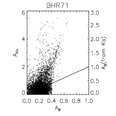
Figure 10: Uncorrected comparison of extinction from NICE method and 8$\mu$m maps for BHR71 (Left) and L483 (Right). Solid line represents the predicted relationship between A_Ks and A₈.

where $A_{Ks}$ is determined from the near-IR extinction measurement. Figure 10 shows the uncorrected relationship between $A_{Ks}$ to $A_{8\mu m}$ for BHR71 and L483. The deviation of the predicted relationship from the observations clearly illustrates the necessity of applying this method to our sample to determine the level of foreground contamination.

Figure 10 clearly indicates that our initial optical depth measurements from Equation (11) needed to be corrected for extra emission. Our near-IR extinction analysis yields the true optical depth from

$$\frac{I_{obs}}{I_{bg}}=e^{-\tau_{8,Ks}}$$ (15)

which is equivalent to

$$\frac{I_{obs}^{\prime}-I_{fg}}{I_{bg}^{\prime}-I_{fg}}=e^{-\tau_{8,Ks}}.$$ (16)

Solving for $I_{fg}$ and some algebraic manipulation give

$$I_{fg}=\frac{I_{bg}^{\prime}(e^{-\tau_{8}^{\prime}}-e^{-\tau_{8,Ks}})}{1-e^{-\tau_{8,Ks}}}.$$ (17)

This relationship assumes that $I_{fg}$ is nearly constant across the envelope, which is a reasonable assumption for the possible sources of foreground given the relatively small angular size of the envelopes.

We have already described how $I_{bg}^{\prime}$ is measured in the previous section. However, $\tau_{8}^{\prime}$ from Equations 11 and 17 requires some special consideration.

Since the near-IR extinction toward these points is determined using stars, there may be point sources detected at the same position in the 8$\mu$m image which will have a negative value in the optical depth map. This is particularly clear in Figure 6 where some background stars are surrounded by a “hole” in the optical depth map. To ensure that our measurements of $\tau_{8}^{\prime}$ from the 8$\mu$m extinction map are mostly unaffected by stars, we measure the average optical depth in an annulus from 4 to 7 pixels around the star at each position. This does introduce some error if a star is very bright at 8$\mu$m, seen in Figure 11 as points with high $A_{Ks}$ but low $A_{8\mu m}$, but for most points in the envelope this method works well. Additional points with high $A_{Ks}$ and low $A_{8\mu m}$ are likely due to the presence of diffuse emission at 8$\mu$m from scattered light in the outflow cavity, outflow knots, and/or a star(s) falling within the measurement annulus. As a test, we compared the average $A_{Ks}$ in a 15^′′ box to the median 8$\mu$m extinction in the same box and the points with high $A_{Ks}$ and low $A_{8\mu m}$ were not present.

We determine $I_{fg}$ by calculating Equation (17) at the position of each near-IR extinction measurement where $A_{Ks}>1$ and $A_{8\mu m}$ is greater than the 1 sigma noise in the uncorrected optical depth map. Then we take the median value of $I_{fg}$ and subtract it from the 8$\mu$m image and recalculate the optical depth map. Then we run the comparison again on the corrected image and $I_{fg}$ should be close to zero; graphically we check to see if the datapoints agree with the predicted relationship, usually $I_{fg}$ will only need to be adjusted slightly from the initial value. We note that the regions of highest $\tau_{8}^{\prime}$/$A_{Ks}$ yield the best value of $I_{fg}$ because the percentage error for these points is the least; there can be significant scatter at low $\tau_{8}^{\prime}$/$A_{Ks}$. As shown in Figure 11, the correction to the optical depth measurements results in reasonable estimates of the foreground contribution. As highlighted in §4 this method lead us to the simplifying conclusion that in all images the darkest part of the envelope is completely opaque within uncertainty limits of the images. This finding enables us to also correct our data which lack near-IR measurements or are not observed against a rich stellar field.

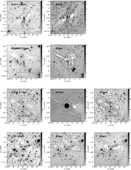
Figure 1: IRAC images of our sample of envelopes with flattened morphology. Left: IRAC 3.6 $\mu$m or Ks-band images which highlight the scattered light cavities in these objects. Middle: IRAC 8.0 $\mu$m images with the 8.0 $\mu$m optical depth contours overlaid. Right: IRAC 8.0 $\mu$m images with SCUBA 850 $\mu$m contours. The line drawn in the left panel corresponds to 0.1 pc at the adopted distance. For HH108, we show the Ks-band image (left), 24$\mu$m image with 24$\mu$m optical depth contours (middle) highlighting structure, and SCUBA 850$\mu$m data overlaid on the Ks-band image (right). The 8.0 $\mu$m optical depth contours correspond to $\tau_{8\mu m}$ values for BHR71: 0.6, 1.28, 2.75; L723: 0.2, 0.3, 0.45; L673: 0.3, 0.6, 1.2; SerpMMS3: 0.75 1.06 1.5; L1157: 0.5, 1.09, 2.4.

Fig. 1 —

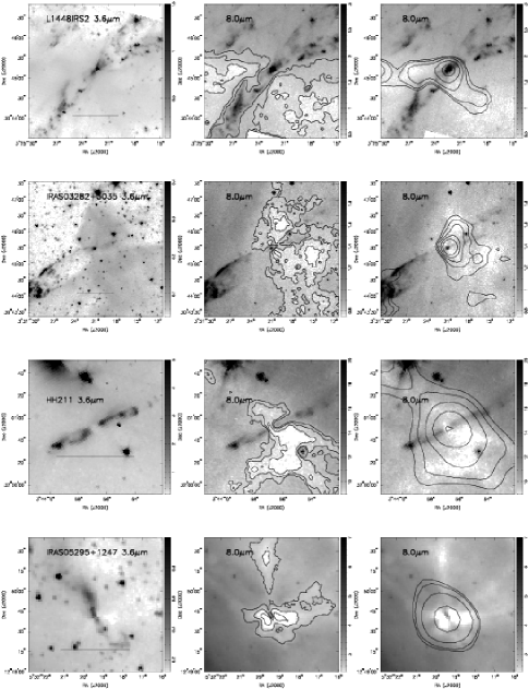
Figure 5: Same as Figure 1 except irregular envelopes are shown. The 8.0 $\mu$m optical depth contours correspond to the following values of $\tau_{8\mu m}$ for L1448 IRS2: 0.6, 1.02, 1.75; IRAS 03282+3035: 0.9, 1.34,2.0; HH211 0.3, 0.57, 1.1; IRAS 05295+1247 0.275, 0.74, 2.0; IRS09449-5052: 0.25, 0.56, 1.25; L483: 0.5, 0.82, 1.35; L1165: 0.3, 0.54, 1.0.

Fig. 5 —

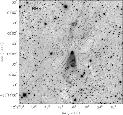
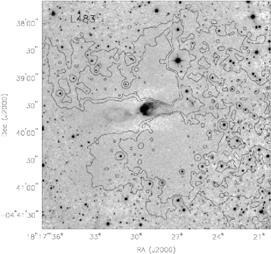
Figure 6: Ks-band images of BHR71 and L483 with the two highest optical depth contours from Figures 1 and 5 overlaid. As detailed in the text and Appendix, a number of background stars in the near-IR can be detected through the dense envelope enabling the correction of the 8$\mu$m optical depth maps. The BHR71 image was taken with ISPI and the smaller PANIC image is inserted at the center. The L483 data was taken with TIFKAM at MDM observatory.

Figure 7: Plots of scale height versus radius for flattened envelopes. The diamonds are the measured scale heights determined by fitting Gaussians to the data, the plus signs are the predicted scale height of an infinite filament with peak surface density computed from the peak optical depth, asterisks are the computed scale heights for a sheet. In the case of filaments and sheets, the scale height computed in §3 does not correspond to the scale height of a Gaussian, to correct for this we integrated through a filament and fit a Gaussian to the surface density profile. The Gaussian scale height is always $\sim$1.5 $\times$ H.

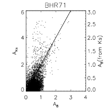
Figure 11: Comparison of extinction from NICE method and corrected 8$\mu$m maps for BHR71 (Left) and L483 (Right). The points with high A_Ks and low A₈ for BHR71 are likely due to a bright 8$\mu$m star at the location of the near-IR measurement or scattered light and outflow emission at 8$\mu$m coincident with the near-IR measurement.

Table 1: Spitzer IRAC Observations

Designation	RA	Dec.	Date(s) Obs.	Int. Time	AORKEY/Program	Near-IR data
	(J2000)	(J2000)		(s)		(Obs./Inst.)
L1448 IRS2	03 25 22.5	$+$30 45 10.5	2005-02-25	900	12250624/P03557
Perseus 5	03 29 51.6	$+$31 39 04	2005-01-29	900	12249344/P03557
IRAS 03282$+$3035	03 31 21.0	$+$30 45 28	2006-09-28	900	18326016/P30516
HH211-mm	03 43 56.8	+32 00 52	2004-08-09	24	5790976
IRAM 04191	04 21 56.9	$+$15 29 46.1	2005-09-18	480	14617856, 14618112
L1521F	04 28 39	$+$26 51 35	2006-03-25	480	14605824, 14605568
L1527	04 35 53.9	$+$26 03 09.7	2004-03-07	90	3963648
IRAS 05295$+$1247	05 32 19.4	$+$12 49 41	2006-10-26	900	18325248/P30516
HH270 VLA1	05 51 34.5	$+$02 56 48	2005-03-25	360	10737920
IRAS 09449-5052	09 46 46.5	-51 06 07	2004-04-29	48	5105152	CTIO/ISPI
BHR71	12 01 37.1	-65 08 54	2004-06-10	150	5107200	Magellan/PANIC, CTIO/ISPI
IRAS 16253-2429	16 28 22.2	-24 36 31	2004-03-29	48	5762816, 5771264
L483	18 17 35	-04 39 48	2004-09-02,03	48	5149184,5149696	MDM/TIFKAM
Serp-MMS3	18 29 09.1	+00 31 28.6	2004-04-05	48	5710848, 5712384
HH108	18 35 44.2	-00 33 15	2007-05-17	Med. Scan	14510336	CTIO/ISPI
L723	19 17 53.2	$+$19 12 16.6	2006-09-27	900	18326528/P30516	MDM/TIFKAM
L673-SMM2	19 20 26.3	+11 20 04	2004-04-30,22	48	5152256, 5151744
L1157	20 39 06.2	$+$68 02 17.3	2006-08-13	900	18324224/P30516	MDM/TIFKAM
L1152	20 35 46.5	$+$67 53 04.2	2004-07-23,28	360	11390976, 11399424	MDM/TIFKAM
CB230	21 17 38.7	$+$68 17 32.9	2004-11-28	60	12548864
L1165	22 06 51.0	$+$59 02 43.5	2004-07-03	48	5165056	MDM/TIFKAM
CB244	23 25 46.5	+74 17 39	2003-12-23	150	4928256	MDM/TIFKAM

Note. —

Table 2: Source Properties

Designation	Distance	Mass	Mass	Mass	Massobs	Lbol	$\sigma\tau$	$\tau_{max}$	$I_{bg}^{\prime}$	$I_{fg}$	Classification	References
	(pc)	($M_{\sun}$)	($M_{\sun}$)	($M_{\sun}$)	($M_{\sun}$)	($L_{\sun}$)			(MJy/sr)	(MJy/sr)		(Mobs, Lbol)
		(r$<$0.15pc)	(r$<$0.1pc)	(r$<$0.05pc)
L1448 IRS2	300	23.0	9.8	2.1	0.86	8.4	0.15	2.35	3.98	3.44	Flattened	13,1
Perseus 5	300	19.2	9.8	3.4	1.24	0.46	0.15	2.3	4.04	3.56	One-sided	3,2
IRAS 03282+3035	300	25.7	14.2	4.0	2.2	1.2	0.3	2.1	2.55	2.26	Irregular	4,2
HH211	300	5.5	3.4	1.8	1.5	3.02	0.15	1.7	10.1	8.57	Irregular	3,3
IRAM 04191	140	9.7	6.1	1.0	…	0.3	0.22	0.9	4.09	3.77	Spheroidal	..,7
L1521F	140	5.9	4.8	2.3	…	0.03	0.35	1.2	4.65	4.35	Spheroidal	..,8
L1527	140	1.9	1.5	0.84	2.4	2.0	0.2	1.5	4.37	4.0	One-sided	5,9
IRAS 05295+1247	400	2.9	2.4	1.5	…	12.5	0.05	3.3	5.2	4.02	Irregular	..,1
HH270 VLA1	420	7.8	5.7	1.9	…	7.0	0.12	2.4	4.2	3.72	One-sided	..,1
IRAS 09449-5052	300?	4.7	3.6	1.8	3.7	3.1	0.25	1.25	2.46	2.1	Irregular	6,6
BHR71	200	24.5	13.8	4.6	2.2	9.0	0.1	2.8	4.36	2.3	Flattened	6,6
IRAS 16253-2429	125	5.63	2.9	0.8	0.98	0.25	0.1	1.4	7.0	4.52	Spheroidal	10,2
L483	200	21.5	13.2	3.5	1.8	11.5	0.25	1.75	2.87	2.35	Irregular	4,1
Serp-MMS3	225	3.1	1.3	0.3	2.2	1.6	0.1	2.20	3.93	1.48	Flattened	2, 15
HH108	300				4.5, 3.6	$\sim$8.0, 1.0					Flattened	14
L723	300	4.0	2.1	0.6	1.6	4.6	0.03	3.1	3.22	2.55	Flattened	4,1
L673-SMM2	300	5.2	3.2	1.0	0.35	2.8	0.1	3.6	9.39	3.33	Flattened	12
L1157	250	12.0	6.0	0.6	2.2	3.0	0.1	2.5	0.71	0.45	Flattened	4,1
L1152	250	14.1	7.8	2.4	12.0	1.3	0.15	1.85	0.32	0.18	Binary Core	5,1
CB230	300	7.2	4.1	1.1	1.1	7.2	0.23	1.9	1.79	1.17	One-sided	11,1
L1165	300	6.9	3.8	1.1	0.32	28	0.1	3.0	3.76	2.6	Irregular	12,12
CB244	250	9.7	7.8	4.1	…	…	0.2	1.75	0.59	0.35	Binary Core	..,..

Note. — For HH108 the quoted values are given for IRS1 and IRS2 respectively. References: (1) This work, (2) Enoch et al. (2009), (3)Enoch et al. (2006), (4) Shirley et al. (2000), (5) Benson & Myers (1989), (6) Bourke et al. (1995), (7) Dunham et al. (2006) (8) Terebey et al. (2009), (9) Tobin et al. (2008), (10) Young et al. (2006), (11) Kauffmann et al. (2008) (12) Visser et al. (2002), (13) O’Linger et al. (1999), (14) Chini et al. (2001), (15) Enoch et al. (2007).

Table 3: Moment of Inertia Ratios

Object	Radius	$I_{\perp}$/$I_{\parallel}$	$I_{\perp,l}$/$I_{\perp,r}$	$I_{\parallel,l}$/$I_{\parallel,r}$
	(pc)
Perseus 5	0.05	1.2	1.2	1.0
L1448 IRS2	0.05	0.6	1.0	1.7
IRAS 03282+3035	0.05	1.2	1.0	0.8
HH211	0.05	2.2	0.2	0.2
L1448-IRS2	0.05	1.7	0.6	1.0
IRAM 04191	0.03	1.5	2.5	1.2
L1521F	0.04	1.3	0.9	1.0
L1527	0.05	3.2	0.1	0.1
IRAS 05295+1247	0.05	1.3	0.5	0.5
HH270 VLA1	0.10	0.6	1.4	2.6
IRAS 09449-5052	0.05	1.7	0.8	1.0
BHR71	0.075	1.6	1.1	0.8
IRAS 16253-2429	0.05	1.1	0.9	1.0
L483	0.05	1.4	1.0	0.9
Serp-MMS3	0.05	1.0	1.9	1.5
L723	0.05	1.2	0.8	0.9
L673-SMM2	0.05	0.9	0.1	0.4
L1157	0.05	3.0	0.9	0.8
L1152	0.05	0.8	1.4	1.5
CB230	0.05	3.4	0.3	0.6
L1165	0.05	2.3	0.5	0.8

Note. — $I_{\perp}$ measures material that is located away from the outflow/rotation axis along the abscissa and $I_{\parallel}$ measures material located along the ordinate axis. CB244 does not appear in this table because most extinction in this system is associated with the neighboring starless core, not the protostar.

References

- Adams et al. (1987) Adams, F. C., Lada, C. J., & Shu, F. H. 1987, ApJ, 312, 788
- Alves et al. (2001) Alves, J. F., Lada, C. J., & Lada, E. A. 2001, Nature, 409, 159
- Andrews & Williams (2007) Andrews, S. M., & Williams, J. P. 2007, ApJ, 659, 705
- Anglada et al. (1989) Anglada, G., Rodriguez, L. F., Torrelles, J. M., Estalella, R., Ho, P. T. P., Canto, J., Lopez, R., & Verdes-Montenegro, L. 1989, ApJ, 341, 208
- Arce & Sargent (2006) Arce, H. G., & Sargent, A. I. 2006, ApJ, 646, 1070
- Bachiller et al. (1993) Bachiller, R., Martin-Pintado, J., & Fuente, A. 1993, ApJ, 417, L45
- Bacmann et al. (2000) Bacmann, A., André, P., Puget, J.-L., Abergel, A., Bontemps, S., & Ward-Thompson, D. 2000, A&A, 361, 555
- Ballesteros-Paredes et al. (1999) Ballesteros-Paredes, J., Hartmann, L., & Vázquez-Semadeni, E. 1999, ApJ, 527, 285
- Ballesteros-Paredes et al. (2007) Ballesteros-Paredes, J., Klessen, R. S., Mac Low, M.-M., & Vazquez-Semadeni, E. 2007, Protostars and Planets V, 63
- Basu & Mouschovias (1994) Basu, S., & Mouschovias, T. C. 1994, ApJ, 432, 720
- Basu & Ciolek (2004) Basu, S., & Ciolek, G. E. 2004, ApJ, 607, L39
- Basu et al. (2009) Basu, S., Ciolek, G. E., Dapp, W. B., & Wurster, J. 2009, New Astronomy, 14, 483
- Ciolek & Basu (2006) Ciolek, G. E., & Basu, S. 2006, ApJ, 652, 442
- Bate et al. (2003) Bate, M. R., Bonnell, I. A., & Bromm, V. 2003, MNRAS, 339, 577
- Benson & Myers (1989) Benson, P. J., & Myers, P. C. 1989, ApJS, 71, 89
- Bertin et al. (2002) Bertin, E., Mellier, Y., Radovich, M., Missonnier, G., Didelon, P., & Morin, B. 2002, Astronomical Data Analysis Software and Systems XI, 281, 228
- Bonnell & Bastien (1993) Bonnell, I., & Bastien, P. 1993, ApJ, 406, 614
- Boss (1995) Boss, A. P. 1995, Revista Mexicana de Astronomia y Astrofisica Conference Series, 1, 165
- Bourke et al. (1995) Bourke, T. L., Hyland, A. R., Robinson, G., James, S. D., & Wright, C. M. 1995, MNRAS, 276, 1067
- Bourke (2001) Bourke, T. L. 2001, ApJ, 554, L91
- Burkert & Bodenheimer (1993) Burkert, A., & Bodenheimer, P. 1993, MNRAS, 264, 798
- Burkert & Hartmann (2004) Burkert, A., & Hartmann, L. 2004, ApJ, 616, 288
- Butler & Tan (2008) Butler, M. J., & Tan, J. C. 2008, arXiv:0812.2882
- Caselli et al. (2002) Caselli, P., Benson, P. J., Myers, P. C., & Tafalla, M. 2002, ApJ, 572, 238
- Chandler & Richer (2000) Chandler, C. J., & Richer, J. S. 2000, ApJ, 530, 851
- Chiang et al. (2008) Chiang, H.-F., Looney, L. W., Tassis, K., Mundy, L. G., & Mouschovias, T. C. 2008, ApJ, 680, 474
- Chiang et al. (2009) Chiang, H., Looney, L. W.,Tobin, J. J., Hartmann, L. 2010, ApJ, in press.
- Chen et al. (2007) Chen, X., Launhardt, R., & Henning, T. 2007, ApJ, 669, 1058
- Chini et al. (2001) Chini, R., Ward-Thompson, D., Kirk, J. M., Nielbock, M., Reipurth, B., & Sievers, A. 2001, A&A, 369, 155
- Di Francesco et al. (2001) Di Francesco, J., Myers, P. C., Wilner, D. J., Ohashi, N., & Mardones, D. 2001, ApJ, 562, 770
- Di Francesco et al. (2008) Di Francesco, J., Johnstone, D., Kirk, H., MacKenzie, T., & Ledwosinska, E. 2008, ApJS, 175, 277
- Draine & Li (2001) Draine, B. T., & Li, A. 2001, ApJ, 551, 807
- Dunham et al. (2006) Dunham, M. M., et al. 2006, ApJ, 651, 945
- Dunham et al. (2008) Dunham, M. M., Crapsi, A., Evans, N. J., II, Bourke, T. L., Huard, T. L., Myers, P. C., & Kauffmann, J. 2008, ApJS, 179, 249
- Dunham et al. (2010) Dunham, M. M., Evans, N. J., Terebey, S., Dullemond, C. P., & Young, C. H. 2010, ApJ, 710, 470
- Djupvik et al. (2006) Djupvik, A. A., André, P., Bontemps, S., Motte, F., Olofsson, G., Gålfalk, M., & Florén, H.-G. 2006, A&A, 458, 789
- Elmegreen (2000) Elmegreen, B. G. 2000, ApJ, 530, 277
- Enoch et al. (2006) Enoch, M. L., et al. 2006, ApJ, 638, 293
- Enoch et al. (2007) Enoch, M. L., Glenn, J., Evans, N. J., II, Sargent, A. I., Young, K. E., & Huard, T. L. 2007, ApJ, 666, 982
- Enoch et al. (2009) Enoch, M. L., Evans, N. J., Sargent, A. I., & Glenn, J. 2009, ApJ, 692, 973
- Evans et al. (2001) Evans, N. J., II, Rawlings, J. M. C., Shirley, Y. L., & Mundy, L. G. 2001, ApJ, 557, 193
- Evans et al. (2003) Evans, N. J., II, et al. 2003, PASP, 115, 965
- Evans et al. (2009) Evans, N. J., et al. 2009, ApJS, 181, 321
- Fatuzzo & Adams (2002) Fatuzzo, M., & Adams, F. C. 2002, ApJ, 570, 210
- Galli & Shu (1993) Galli, D., & Shu, F. H. 1993, ApJ, 417, 220
- Galli et al. (2006) Galli, D., Lizano, S., Shu, F. H., & Allen, A. 2006, ApJ, 647, 374
- Girart et al. (1997) Girart, J. M., Estalella, R., Anglada, G., Torrelles, J. M., Ho, P. T. P., & Rodriguez, L. F. 1997, ApJ, 489, 734
- Goodman et al. (1998) Goodman, A. A., Barranco, J. A., Wilner, D. J., & Heyer, M. H. 1998, ApJ, 504, 223
- Fiedler & Mouschovias (1992) Fiedler, R. A., & Mouschovias, T. C. 1992, ApJ, 391, 199
- Flaherty et al. (2007) Flaherty, K. M., Pipher, J. L., Megeath, S. T., Winston, E. M., Gutermuth, R. A., Muzerolle, J., Allen, L. E., & Fazio, G. G. 2007, ApJ, 663, 1069
- Froebrich (2005) Froebrich, D. 2005, ApJS, 156, 169
- Fuller & Wootten (2000) Fuller, G. A., & Wootten, A. 2000, ApJ, 534, 854
- Fűrész et al. (2006) Fűrész, G., et al. 2006, ApJ, 648, 1090
- Fűrész et al. (2008) Fűrész, G., Hartmann, L. W., Megeath, S. T., Szentgyorgyi, A. H., & Hamden, E. T. 2008, ApJ, 676, 1109
- Furlan et al. (2008) Furlan, E., et al. 2008, ApJS, 176, 184
- Hartmann et al. (1994) Hartmann, L., Boss, A., Calvet, N., & Whitney, B. 1994, ApJ, 430, L49
- Hartmann et al. (1996) Hartmann, L., Calvet, N., & Boss, A. 1996, ApJ, 464, 387
- Hartmann (2002) Hartmann, L. 2002, ApJ, 578, 914
- Hartmann (2009) Hartmann, L. 2009, Accretion processes in star formation / Lee Hartmann. Cambridge, UK ; New York : Cambridge University Press, 2009. (Cambridge astrophysics series ; 47) ISBN 0521531993.,
- Harvey et al. (2003) Harvey, D. W. A., Wilner, D. J., Lada, C. J., Myers, P. C., & Alves, J. F. 2003, ApJ, 598, 1112
- Heitsch et al. (2008a) Heitsch, F., Hartmann, L. W., Slyz, A. D., Devriendt, J. E. G., & Burkert, A. 2008a, ApJ, 674, 316
- Heitsch et al. (2001) Heitsch, F., Mac Low, M.-M., & Klessen, R. S. 2001, ApJ, 547, 280
- Heitsch & Hartmann (2008) Heitsch, F., & Hartmann, L. 2008, ApJ, 689, 290
- Heitsch et al. (2008b) Heitsch, F., Hartmann, L. W., & Burkert, A. 2008b, ApJ, 683, 786
- Indebetouw et al. (2005) Indebetouw, R., et al. 2005, ApJ, 619, 931
- Johnstone et al. (2003) Johnstone, D., Fiege, J. D., Redman, R. O., Feldman, P. A., & Carey, S. J. 2003, ApJ, 588, L37
- Jones et al. (2001) Jones, C. E., Basu, S., & Dubinski, J. 2001, ApJ, 551, 387
- Jørgensen (2004) Jørgensen, J. K. 2004, A&A, 424, 589
- Jørgensen et al. (2007) Jørgensen, J. K., et al. 2007, ApJ, 659, 479
- Kauffmann et al. (2008) Kauffmann, J., Bertoldi, F., Bourke, T. L., Evans, N. J., II, & Lee, C. W. 2008, A&A, 487, 993
- Kirk et al. (2009) Kirk, J. M., Crutcher, R. M., & Ward-Thompson, D. 2009, ApJ, 701, 1044
- Kenyon et al. (1993) Kenyon, S. J., Calvet, N., & Hartmann, L. 1993, ApJ, 414, 676
- Klessen & Burkert (2000) Klessen, R. S., & Burkert, A. 2000, ApJS, 128, 287
- Klessen et al. (2000) Klessen, R. S., Heitsch, F., & Mac Low, M.-M. 2000, ApJ, 535, 887
- Kratter et al. (2009) Kratter, K. M., Matzner, C. D., Krumholz, M. R., & Klein, R. I. 2009, arXiv:0907.3476
- Kunz & Mouschovias (2009) Kunz, M. W., & Mouschovias, T. C. 2009, ApJ, 693, 1895
- Kwon et al. (2009) Kwon, W., Looney, L. W., Mundy, L. G., Chiang, H.-F., & Kemball, A. J. 2009, ApJ, 696, 841
- Lada et al. (1994) Lada, C. J., Lada, E. A., Clemens, D. P., & Bally, J. 1994, ApJ, 429, 694
- Launhardt et al. (2001) Launhardt, R., Sargent, A., & Zinnecker, H. 2001, Science with the Atacama Large Millimeter Array, 235, 134
- Lee et al. (2004) Lee, J.-E., Bergin, E. A., & Evans, N. J., II 2004, ApJ, 617, 360
- Lin et al. (1965) Lin, C. C., Mestel, L., & Shu, F. H. 1965, ApJ, 142, 1431
- Loinard et al. (2002) Loinard, L., Rodríguez, L. F., D’Alessio, P., Wilner, D. J., & Ho, P. T. P. 2002, ApJ, 581, L109
- Lombardi & Alves (2001) Lombardi, M., & Alves, J. 2001, A&A, 377, 1023
- Looney et al. (2000) Looney, L. W., Mundy, L. G., & Welch, W. J. 2000, ApJ, 529, 477
- Looney et al. (2007) Looney, L. W., Tobin, J. J., & Kwon, W. 2007, ApJ, 670, L131
- Luhman (2008) Luhman, K. L. 2008, Handbook of Star Forming Regions, Volume II: The Southern Sky ASP Monograph Publications, Vol. 5. Edited by Bo Reipurth, p.169, 169
- Mac Low & Klessen (2004) Mac Low, M.-M., & Klessen, R. S. 2004, Reviews of Modern Physics, 76, 125
- Meadows et al. (2004) Meadows, V. S., et al. 2004, ApJS, 154, 469
- McClure (2009) McClure, M. 2009, ApJ, 693, L81
- Mink (1999) Mink, D. J. 1999, Astronomical Data Analysis Software and Systems VIII, 172, 498
- Maury et al. (2010) Maury, A. J., et al. 2010, arXiv:1001.3691
- Myers et al. (1991) Myers, P. C., Fuller, G. A., Goodman, A. A., & Benson, P. J. 1991, ApJ, 376, 561
- Myers et al. (1998) Myers, P. C., Adams, F. C., Chen, H., & Schaff, E. 1998, ApJ, 492, 703
- Offner & Krumholz (2009) Offner, S. S. R., & Krumholz, M. R. 2009, ApJ, 693, 914
- O’Linger et al. (1999) O’Linger, J., Wolf-Chase, G., Barsony, M., & Ward-Thompson, D. 1999, ApJ, 515, 696
- Padoan et al. (2001) Padoan, P., Juvela, M., Goodman, A. A., & Nordlund, Å. 2001, ApJ, 553, 227
- Pogge et al. (1998) Pogge, R. W., et al. 1998, Proc. SPIE, 3354, 414
- Padoan & Nordlund (2002) Padoan, P., & Nordlund, Å. 2002, ApJ, 576, 870
- Pagani et al. (2009) Pagani, L., Daniel, F., & Dubernet, M.-L. 2009, A&A, 494, 719
- Pineda et al. (2010) Pineda, J. E., et al. 2010, ApJsubmitted.
- Ragan et al. (2009) Ragan, S. E., Bergin, E. A., & Gutermuth, R. A. 2009, arXiv:0903.2771
- Reach et al. (2005) Reach, W. T., et al. 2005, PASP, 117, 978
- Rieke & Lebofsky (1985) Rieke, G. H., & Lebofsky, M. J. 1985, ApJ, 288, 618
- Román-Zúñiga et al. (2007) Román-Zúñiga, C. G., Lada, C. J., Muench, A., & Alves, J. F. 2007, ApJ, 664, 357
- Ryden (1996) Ryden, B. S. 1996, ApJ, 471, 822
- Seale & Looney (2008) Seale, J. P., & Looney, L. W. 2008, ApJ, 675, 427
- Shirley et al. (2000) Shirley, Y. L., Evans, N. J., II, Rawlings, J. M. C., & Gregersen, E. M. 2000, ApJS, 131, 249
- Shu (1977) Shu, F. H. 1977, ApJ, 214, 488
- Shu et al. (1994) Shu, F., Najita, J., Ostriker, E., Wilkin, F., Ruden, S., & Lizano, S. 1994, ApJ, 429, 781
- Shu et al. (2007) Shu, F. H., Galli, D., Lizano, S., Glassgold, A. E., & Diamond, P. H. 2007, ApJ, 665, 535
- Simon et al. (2006) Simon, R., Jackson, J. M., Rathborne, J. M., & Chambers, E. T. 2006, ApJ, 639, 227
- Spitzer (1968) Spitzer, L., Jr. 1968, Nebulae and interstellar matter. Edited by Barbara M. Middlehurst; Lawrence H. Aller. Library of Congress Catalog Card Number 66-13879. Published by the University of Chicago Press, Chicago, ILL USA, 1968, p.1, 1
- Stark et al. (2006) Stark, D. P., Whitney, B. A., Stassun, K., & Wood, K. 2006, ApJ, 649, 900
- Stutz et al. (2008) Stutz, A. M., et al. 2008, ApJ, 687, 389
- Stutz et al. (2009) Stutz, A. M., et al. 2009, ApJ, in prep.
- Tassis & Mouschovias (2007) Tassis, K., & Mouschovias, T. C. 2007, ApJ, 660, 370
- Terebey et al. (1984) Terebey, S., Shu, F. H., & Cassen, P. 1984, ApJ, 286, 529
- Terebey et al. (2009) Terebey, S., et al. 2009, ApJ, 696, 1918
- Tobin et al. (2007) Tobin, J. J., Looney, L. W., Mundy, L. G., Kwon, W., & Hamidouche, M. 2007, ApJ, 659, 1404
- Tobin et al. (2008) Tobin, J. J., Hartmann, L., Calvet, N., & D’Alessio, P. 2008, ApJ, 679, 1364
- Tobin et al. (2009) Tobin, J. J., Hartmann, L., Furesz, G., Mateo, M., & Megeath, S. T. 2009, arXiv:0903.2775
- van der Bliek et al. (2004) van der Bliek, N. S., et al. 2004, Proc. SPIE, 5492, 1582
- Visser et al. (2002) Visser, A. E., Richer, J. S., & Chandler, C. J. 2002, AJ, 124, 2756
- Walch et al. (2009) Walch, S., Naab, T., Burkert, A., Whitworth, A., & Gritschneder, M. 2009, arXiv:0908.2443
- Weingartner & Draine (2001) Weingartner, J. C., & Draine, B. T. 2001, ApJ, 548, 296
- Whitney & Hartmann (1993) Whitney, B. A., & Hartmann, L. 1993, ApJ, 402, 605
- Whitney et al. (2003) Whitney, B. A., Wood, K., Bjorkman, J. E., & Wolff, M. J. 2003, ApJ, 591, 1049
- Whitney et al. (2005) Whitney, B. A., Robitaille, T. P., Indebetouw, R., Wood, K., Bjorkman, J. E., & Denzmore, P. 2005, Massive Star Birth: A Crossroads of Astrophysics, 227, 206
- Young et al. (2006) Young, K. E., et al. 2006, ApJ, 644, 326