Locating the VHE source in the Galactic Centre with milli-arcsecond accuracy

Abstract

Very high-energy $\gamma$-rays (VHE; E$>$100 GeV) have been detected from the direction of the Galactic Centre up to energies E$>$10 TeV. Up to now, the origin of this emission is unknown due to the limited positional accuracy of the observing instruments. One of the counterpart candidates is the super-massive black hole (SMBH) Sgr A^∗. If the VHE emission is produced within $\approx 10^{15}$ cm $\approx 1000\ r_{G}$ ($r_{G}=GM/c^{2}$ is the Schwarzschild radius) of the SMBH, a decrease of the VHE photon flux in the energy range 100–300 GeV is expected whenever an early type or giant star approaches the line of sight within $\approx$ milli-arcseconds (mas). The dimming of the flux is due to absorption by pair-production of the VHE photons in the soft photon field of the star, an effect we refer to as pair-production eclipse (PPE). Based upon the currently known orbits of stars in the inner arcsecond of the Galaxy we find that PPEs lead to a systematic dimming in the 100–300 GeV band at the level of a few per cent and lasts for several weeks. Since the PPE affects only a narrow energy band and is well correlated with the passage of the star, it can be clearly discriminated against other systematic or even source-intrinsic effects. While the effect is too small to be observable with the current generation of VHE detectors, upcoming high count-rate experiments like the Cherenkov telescope array (CTA) will be sufficiently sensitive. Measuring the temporal signature of the PPE bears the potential to locate the position and size of the VHE emitting region within the inner 1000 $r_{G}$ or in the case of a non-detection exclude the immediate environment of the SMBH as the site of $\gamma$-ray production altogether.

1 Introduction

The central region of our Galaxy harbours a super-massive black hole (SMBH) with a mass $M=(4.31\pm 0.06_{|\,\mathrm{stat}}\pm 0.36_{\,|R_{0}})\times 10^{6}M_{\odot}$ at a distance from Earth of $R_{0}=8.33\pm 0.35$ kpc (Gillessen et al. 2009). Its proximity enables detailed observations with high angular resolution in the radio and, recently by the use of adaptive optics, in the near infrared band (for a review see e.g. Reid 2009). Accurate measurement of the Keplerian orbits of stars in the inner arcsecond of the Galactic Centre (Schödel et al., 2002; Ghez et al., 2003; Eisenhauer et al., 2005; Gillessen et al., 2009) has revealed the presence of a compact massive object co-located with the radio-source Sgr A^∗ (Balick & Brown, 1974; Reid et al., 2007). The astrometry allows for a shift of up to 2 mas (Gillessen et al., 2009) being the upper limit on the systematic error of the position between the radio and near infrared positions of Sgr A^∗.

Recently, very high-energy (VHE; E$>$100 GeV) emission has been detected from the Galactic Centre region (Aharonian et al., 2004; Kosack et al., 2004; Tsuchiya et al., 2004; Albert et al., 2006). A number of different scenarios for particle acceleration and $\gamma$-ray production have been discussed in the literature. Aharonian & Neronov (2005) have considered $\gamma$-ray production both from electrons via curvature radiation as well as from hadronic processes (photo-meson production and proton-proton scattering). The energetic photons can be produced as close as 20 $r_{G}$ without suffering strong absorption via pair-production with the photon field generated by the low-luminosity SMBH ($L<10^{-8}~{}L_{\mathrm{Edd}}$) (Aharonian & Neronov, 2005). In another SMBH-related scenario suggested by Atoyan & Dermer (2004) an assumed relativistic wind injected in the vicinity of the SMBH would lead to the formation of a synchrotron/inverse-Compton nebula similar to pulsar wind generated nebulae. In this case the VHE emission would be produced in the vicinity of the shock that is leading to acceleration of particles at a distance of $\mathcal{O}(10^{16})$ cm to the SMBH. More production scenarios, which are not directly related to the SMBH, have been discussed: The pulsar-wind nebula candidate G359.95-0.04 (Wang et al., 2006), the stellar cluster IRS 13 (Maillard et al., 2004), the low-mass X-ray binary candidate J174540.0-290031, Sgr A East (Aharonian et al., 2006a) or self-annihilating Dark Matter (see e.g. Horns 2005). Fig. 1 shows an X-ray image (0.3–8 keV) derived from 156 hours of archival Chandra observations including the X-ray emission observed from the various counterpart candidates located within the location uncertainty of the VHE source.

Recent improved reconstruction of the location of the VHE-source (Acero et al., 2009) has excluded the emission originating predominantly from Sgr A East, while the other possibilities mentioned above remain viable.

The absence of flux variability in the VHE band during simultaneous observations of Sgr A^∗ by H.E.S.S. (High Energy Stereoscopic Systme) and Chandra seem to disfavour a common origin of the X-ray and the VHE emission, yet such a scenario can not be excluded (Aharonian et al., 2008).

Despite the efforts to reduce the positional error of the VHE source, the current uncertainty of 6 arcsec (syst.) per telescope axis (Acero et al., 2009) is limited to systematic errors. The prospects for a substantial improvement on the systematic uncertainties are limited by the mechanical stability of air Cherenkov telescopes, which would require substantial improvement with respect to the currently used light-weight construction. The Galactic Centre region is too crowded to identify the VHE source reliably. Unless a clear timing signature can be established, this will not change.

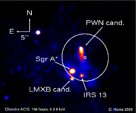
Figure 1: Chandra X-ray image of the Galactic Centre region accumulated from 156 hours of data in the 0.3–8 keV band. The possible sources for the VHE emission are marked, the small circle indicates the position of the H.E.S.S. source ($l=359^{\circ}56^{\prime}41.1^{\prime\prime}\pm 6.4^{\prime\prime}$ (stat.), $b=-0^{\circ}2^{\prime}39.2^{\prime\prime}\pm 5.9^{\prime\prime}$ (stat.)) as reported in Acero et al. (2009). The large white ellipse marks the combined statistical and systematical (6 arcsec) H.E.S.S. positional uncertainty region. The supernova candidate Sgr A East is outside of the image.

In this paper we propose the use of a time-dependent attenuation feature, which provides a novel opportunity to constrain the size and location of the Galactic Centre VHE-source with an accuracy of milli-arcseconds in the case of the VHE emission being produced in the vicinity of Sgr A^∗. We provide a long-term (60 yrs) prediction of flux variations in different energy bands which can be caused by the passage of stars close to the line of sight towards the VHE source.

2 Pair-production eclipses

In the following we assume that VHE $\gamma$-rays originate from a region near the SMBH Sgr A^∗. These VHE photons interact with soft photon fields via the pair-production process ($\gamma_{\mathrm{{VHE}}}+\gamma_{*}\rightarrow e^{+}+e^{-}$). Stars on stable Keplerian orbits in the direct vicinity of Sgr A^∗ ($<1^{\prime\prime}$) provide these (low-energy) photon fields, and pair-production can lead to an energy-dependent dimming of the VHE-flux. Since the position of the star changes, the optical depth $\tau$ for the VHE photon varies along the orbit of the star. In the following we will calculate $\tau$ as a function of time and $\gamma$-ray energy for stars on Keplerian orbits.

2.1 Pair-production

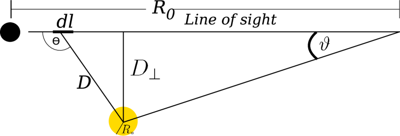
Figure 2: A cartoon of the line of sight integration and the used geometry.

The total cross-section for pair-production (after averaging over polarisation states) is given as

$$\begin{split}\sigma(\varepsilon,E,\theta)&=\frac{3\sigma_{T}}{16}(1-\beta^{2})\\ &\times\left[(3-\beta^{4})\ln\left(\frac{1+\beta}{1-\beta}\right)\ -2\beta(2-\beta^{2})\right],\end{split}$$ (1)

with $\sigma_{T}$ being the Thomson cross-section, $\beta=(1-1/s)^{1/2}$ and $s=\varepsilon E/(2m_{e}^{2}c^{4})(1-\cos\theta)$ the (normalized) centre-of-momentum energy of two photons of energy $\varepsilon$ and $E$ interacting at an angle $\theta$ in the laboratory frame (Gould & Schréder, 1967). We choose the laboratory frame as the system where the VHE source is at rest. The cross-section is strongly energy-dependent and has a maximum for photon energies of

$$E_{\mathrm{max}}=0.9\left(\frac{\varepsilon}{\mathrm{eV}}\right)^{-1}\mathrm{TeV,}$$ (2)

corresponding to a maximal cross-section for a 1 TeV $\gamma$-photon interacting with a 0.9 eV ($\lambda\approx 1.38\ \mathrm{\mu m}$, near infrared) stellar photon. The relative velocities of the observer as well as the star with respect to the VHE source are considered to be small (with respect to the speed of light $c$) and will be neglected in the following. For the considered case we assume the stellar atmosphere of a star with radius $R_{\ast}$ and effective temperature $T_{\mathrm{eff}}$ to be the source of low-energy photons. The differential photon density $dn=n(\varepsilon)~{}d\varepsilon$ at the photosphere of the star can be approximated with a black-body spectrum:

$$n(\varepsilon)=\frac{2\varepsilon^{2}}{h^{3}c^{3}}\left[\exp\left({\frac{\varepsilon}{k_{B}T_{\text{eff}}}}\right)-1\right]^{-1},$$ (3)

with $h$ being Planck’s constant, $c$ the speed of light and $k_{B}$ Boltzmann’s constant. The optical depth for VHE photons with energy $E$ is calculated by integrating along the line of sight subtending a perpendicular distance $D_{\perp}$ to the star (see Fig. 2 for a definition of the geometry):

$$\tau(E)=\int\limits_{0}^{R_{0}}dl\int\limits_{c_{\text{min}}}^{1}d\cos{\Theta}\int\limits_{0}^{2\pi}d\phi\int\limits_{\varepsilon_{\text{min}}}^{\infty}d\varepsilon\ \sigma(\varepsilon,E,\theta)\ n(\varepsilon)\ (1-\cos{\theta}),$$ (4)

with $c_{\mathrm{min}}=\left[1-\left(\frac{R_{\ast}}{D}\right)^{2}\right]^{1/2}$ and $\varepsilon_{\mathrm{min}}=2m_{e}^{2}c^{4}/[E(1-\cos{\theta})]$ being the minimum energy for pair-production to occur (e.g. Dubus, 2006). For $R_{\ast}\ll D$ the integration over the solid angle in Eq. 4 leads to the point-source approximation:

$$\tau(E)=\int\limits_{0}^{R_{0}}dl\int\limits_{\varepsilon_{\mathrm{min}}}^{\infty}d\varepsilon\ \pi\left(\frac{R_{\ast}}{D}\right)^{2}\ \sigma(\varepsilon,E,\theta)\ n(\varepsilon)\ (1-\cos{\theta}).$$ (5)

For the distances examined here this is an appropriate approximation and will be used in the following.

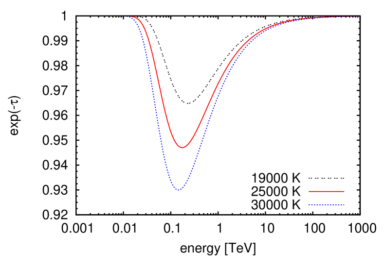
Figure 3: Energy dependence of the absorption $\exp{(-\tau)}$ for a fixed perpendicular angular separation of 1 mas (for a distance $R_{0}=8.33$ kpc). The three curves show the absorption for temperatures $T_{\mathrm{eff}}$ of the star; the stellar radius is adjusted according to the range of stellar types suggested for the well-studied S2 star ($T_{\mathrm{eff}}=19\,000$ K, $R_{\ast}=13.1~{}R_{\odot}$; $T_{\mathrm{eff}}=25\,000$ K, $R_{\ast}=10.7~{}R_{\odot}$; $T_{\mathrm{eff}}=30\,000$ K, $R_{\ast}=9.4~{}R_{\odot}$) (Martins et al., 2008).

In order to demonstrate the uncertainty on the optical depth that results from the uncertainty on the stellar parameters, we calculate the optical depth for the well-studied star “S2”. This star is constrained to have a temperature $19\,000\ \mathrm{K}<T_{\mathrm{eff}}<30\,000\ \mathrm{K}$ and therefore stellar radii $13.1\ R_{\odot}>R_{\ast}>9.4\ R_{\odot}$ (Martins et al., 2008) corresponding to spectral types B0–B2.5V. Fig. 3 shows the result of the calculation of Eq. 5 for a fixed distance $D_{\perp}$ corresponding to a projected angular separation of 1 mas of the VHE source and the star. The absorption shows a pronounced minimum around 200 GeV for $T_{\mathrm{eff}}=19\,000$ K shifting to smaller energies (see also Eq. 2) with increasing stellar temperature. The stellar types have been determined spectroscopically for nearly 50 so-called S-stars. Most stars are early type, B-main-sequence-stars with stellar radii of 10–20 $R_{\odot}$ and effective temperatures of 2–3$\times 10^{4}$ K (Martins et al. 2008).

As shown in Appendix A an additional contribution of cascade radiation coming from the electron/positron pairs produced in the PPE is negligible. The resulting change is similar to the uncertainties resulting from the uncertainties of the orbital elements. Therefore, the effect is generally not of importance.

Another effect which could change the timing signature is a possible change of the accretion flow towards the SMBH induced by the star closely passing Sgr A^∗. Direct wind-driven accretion can lead to an increased accretion rate, but the fast motion of the S-stars does not allow any accretion during periastron passage (Loeb, 2004). Furthermore, the PPE can be treated as independent from accretion induced variability, because it is strongly time- and energy-dependent.

2.2 Stellar orbits and optical depth for VHE photons

The temporal evolution of the optical depth calculated by means of Eq. 5 depends on the position of the star relative to the line of sight, which in turn varies along the orbit of the star. The orbital parameters of 29 stars in the central arcsecond of the Milky Way have been well-measured using both spectroscopy and time-dependent astrometry with unprecedented accuracy utilising the VLT advanced adaptive optics in the near-infrared (K-)band (Eisenhauer et al., 2005; Gillessen et al., 2009).

With the given orbital parameters we derived the three-dimensional position using the known methods described e.g. in Murray & Dermott (1999). The projection of three stellar orbits on the plane of the sky is shown in Fig. 4. The stars S2, S6, and S14 have been selected in particular, because they approach the line of sight closest and therefore are expected to lead to the largest absorption effect. Since the spectral types of these stars are not exactly known, representative values for a B-type main sequence star (similar to the parameters for S2) are used: $R_{\ast}=10.7~{}R_{\odot}$ and $T_{\mathrm{eff}}=2.5\times 10^{4}$ K.

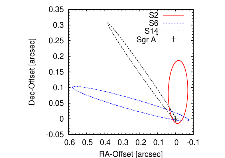
Figure 4: The projected (on the plane of the sky) orbits of three selected S-stars (see text). The cross marks the position of Sgr A^∗.

Table 1: Parameters of selected S-stars: The first 7 columns show the orbital parameters taken from Gillessen et al. (2009), the last two columns list the minimal angular separation of the star to the line of sight $\vartheta$ (in mas) and the resulting maximum absorption $\exp{[-\tau(E)]}$ for $E=200~{}\mathrm{GeV}$.

Star	$a~{}[^{\prime\prime}]$	$e$	$i~{}[^{\circ}]$	$\Omega~{}[^{\circ}]$	$\omega~{}[^{\circ}]$	$t_{P}~{}[yr]$	$T~{}[yr]$	$\vartheta$[mas]	$\exp{(-\tau)}$
S2	$0.123\pm 0.001$	$0.880\pm 0.003$	$135.25\pm 0.47$	$225.39\pm 0.84$	$63.56\pm 0.84$	$2002.32\pm 0.01$	$15.80\pm 0.11$	$10.8\pm 0.4$	$0.9944^{+0.0003}_{-0.0002}$
S6	$0.436\pm 0.153$	$0.886\pm 0.026$	$86.44\pm 0.59$	$83.46\pm 0.69$	$129.5\pm 3.1$	$2063\pm 21$	$105\pm 34$	$3.4\pm 0.9$	$0.966^{+0.002}_{-0.008}$
S14	$0.256\pm 0.010$	$0.963\pm 0.006$	$99.4\pm 1.0$	$227.74\pm 0.70$	$339.0\pm 1.6$	$2000.07\pm 0.06$	$47.3\pm 2.9$	$2.2\pm 0.4$	$0.976^{+0.002}_{-0.003}$

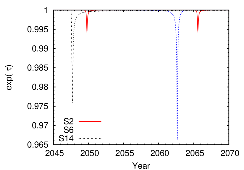
Figure 5: Absorption $\exp[-\tau(E,t)]$ due to pair-production eclipses for three S-stars for VHE photons of energy $E=200$ GeV as function of the calendar year.

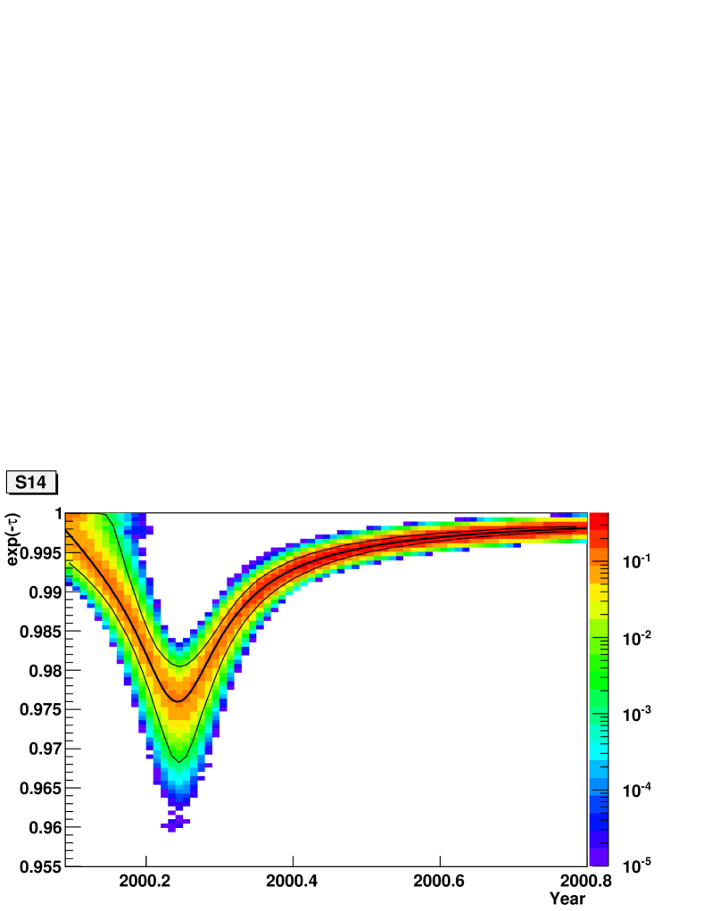
Figure 6: Absorption $\exp[-\tau(E,t)]$ due to pair-production eclipses for the star S14: the curves denote the most likely absorption and the 99 per cent c.l. region. The underlying histogramme indicates the smoothed probability density function resulting from the Monte–Carlo calculations (see text for details).

Table 1 lists the known orbital parameters, their uncertainties, the derived minimal angular separation $\vartheta\approx D_{\perp}/R_{0}$ as well as the correspondingly calculated absorption $\exp(-\tau)$ for VHE photons of energy $E=200$ GeV. The optical depth takes into account the full three-dimensional geometry of the problem. For the three stars considered here the calculated maximum attenuation of the VHE-flux turns out to be 0.5 per cent for S2, 2.4 per cent for S14 and 3.4 per cent for S6. Fig. 5 depicts the predicted absorption of these three stars until the year 2070.

In order to propagate the uncertainties on the orbital parameters into uncertainties on the absorption, a dedicated Monte–Carlo-type simulation has been performed. Since the errors on the different orbital parameters are correlated, we transformed the parameters in the system of the eigenvectors of the covariance matrix and varied these transformed (then uncorrelated) parameters randomly 10 000 times following a normal distribution within the known variance. After back-transforming, we end up with 10 000 orbital parameter-sets tracing the probability density function including the correlation of the parameters.

In order to derive the resulting uncertainty on the absorption effect, we calculated $\exp[-\tau(E,t)]$ for each parameter-set obtained in the Monte–Carlo simulation. As a consequence of the uncertainties of the orbital parameters the time when the minimum of $\exp(-\tau)$ occurs varies considerably. Since we are mainly interested in the uncertainty on the absorption at a fixed time we shifted all curves in time to the mean (best-fitting) value. The most likely attenuation $\exp(-\tau)$ for the star S14 is shown in Fig. 6 together with the 99 per cent confidence interval. For the other stars the uncertainties (68 per cent confidence level) on the minimum of $\exp(-\tau)$ are listed in Table 1. Moreover, the often unknown exact stellar type leads to additional uncertainties on the absorption, which are of similar magnitude as the uncertainties due to the errors on the orbital elements.

2.3 Simulated light curves

The predicted flux modulation due to PPE is at the level of a few per cent (depending on the estimated uncertainties of the orbit and stellar type). In order to investigate the possibility of discovering PPEs measurements of light curves are simulated for future Imaging Air Cherenkov Telescopes (IACTs). For completeness and comparison light curves for the H.E.S.S. telescope system (Hinton, 2004) are simulated as well.

The expected photon rate $R(E_{1},E_{2},t)$ in an energy band $E_{1}$–$E_{2}$ is calculated:

$$R(E_{1},E_{2},t)=\int\limits_{E_{1}}^{E_{2}}dE\ A_{\mathrm{eff}}(E)\phi(E)\ \exp{[-\tau(E,t)]}$$ (6)

with $A_{\mathrm{eff}}(E)$ the effective area of the IACT, $\phi(E)$ the differential VHE photon spectrum from the Galactic Centre, and $\tau(E,t)$ the optical depth calculated by means of Eq. 5. The photon spectrum $\phi(E)$ is assumed to follow a power-law with photon index $2.25$ (Aharonian et al., 2006a). The recently published finding of an exponential cut-off in the energy spectrum at $\approx 16$ TeV (Aharonian et al., 2009) changes the predicted rate between 1 and 10 TeV only marginally and is therefore neglected here.

The effective areas assumed (see Fig. 7) are parameterised based upon Aharonian et al. (2006b) for H.E.S.S. and Punch (2005) for H.E.S.S. II (see Appendix B for further details). For a next generation telescope-system (like the planned CTA, see e.g. Hermann et al. 2008) we generically assumed an increase of the effective area by a factor of 25 with respect to the H.E.S.S. collection area as well as a lower energy threshold of about 10 GeV.

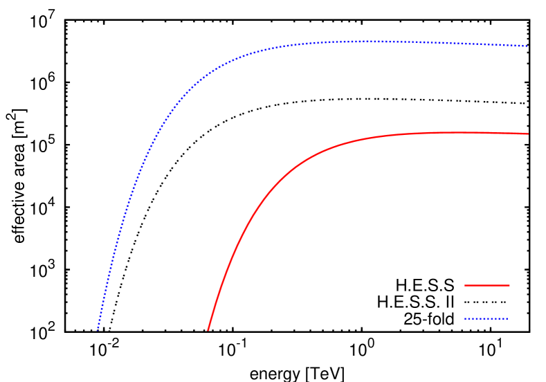
Figure 7: Effective areas for different IACTs used in the simulation of the light curves.

In the following three separate energy bands are considered: the very low energy (10–50 GeV) band, the low energy band (100–300 GeV), and the high energy band (1–10 TeV). Given the energy dependence of the PPE, most of the attenuation will affect the low energy band, whereas the adjacent energy bands remain without attenuation.

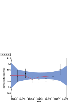
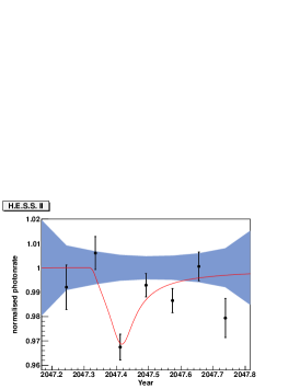
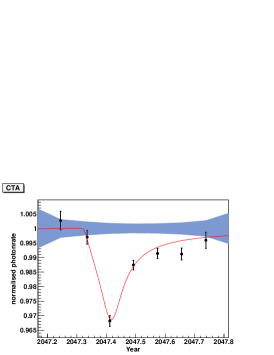
Figure 8: Simulated light-curves for the star S14 for 3 different experiments. The red curve shows the calculated absorption for $E=200$ GeV, the points show the normalised photon-rate in the low energy band (100–300 GeV) where the effect has its maximum. The shaded area marks the photon-rate and its statistical uncertainty without absorption in the combined high (1–10 TeV) and very low (10–50 GeV) energy band. In this band the expected absorption is negligible (see Fig. 3). From left to right: H.E.S.S., H.E.S.S. II, CTA (note: change in scale of the three panels y-axis).

The available observation time is calculated for a site at the Tropic of Capricorn taking into account the dark (moon-less) visibility time of the Galactic Centre between roughly March to September. For each new moon period, the number of detected photons is estimated in the three energy bands by calculating $N_{\mathrm{ph}}(E_{1},E_{2})=R\ t_{\mathrm{vis}}$, with $t_{\mathrm{vis}}$ being the actual observation time available until the Galactic Centre reaches an altitude smaller than 30^∘. The variance on the number of observed photons is estimated under the assumption of Poissonian statistics, and the expected value $N_{\mathrm{ph}}$ is sampled following a normal distribution. This is done separately for the three energy bands. The resulting simulated light curve for the passage of S14 in the year 2047 (normalised to the unattenuated light curve) for the low-energy band for the three IACT setups is shown in the three panels of Fig. 8. In addition to the attenuated low-energy band, the other two energy bands are combined into a comparison measurement marked by the shaded region. This comparison measurement allows the elimination of systematic effects due to observational artefacts or even source intrinsic, broad band variability of the source. It should be noted that the variation of the collection area for different zenith angles has not been included in the calculation. In principle, for smaller altitude angles, the lowest energy band will not be accessible any more. However, this will be compensated by an increase of the collection area at larger energies not altering the conclusions drawn here.

The large uncertainty of the time of the closest approach to the line of sight for S14 ($\approx 3$ yrs) leaves us freedom to shift the light-curve in time. The time of the closest approach is shifted slightly with respect to the best-fit value by 2 months to the middle of the year 2047. In this way the maximum observation time available for Cherenkov telescopes is in phase with the time of the closest approach. Additionally, we assumed the largest possible attenuation of the flux within the orbital uncertainties (see Table 1). Fig. 8 shows that a state of the art IACT like H.E.S.S. (left graph) is not able to detect a PPE within the measurement errors. Under the favourable assumptions used H.E.S.S. II (middle graph) will be able to discover a PPE within the errors. A next generation IACT-system like the planned CTA (right graph) will discover PPEs even under unfavourable conditions.

3 Summary and discussion

Under the assumption that a compact emission region ($<~{}1000~{}r_{G}$) in the vicinity of Sgr A^∗ is the dominant source of the $\gamma$-rays, pair-production eclipses can lead to a time- and energy-dependent dimming of the $\gamma$-ray flux from the direction of the Galactic Centre. Here, we have calculated for the first time the effect of PPEs for the Galactic Centre and provide predictions for the next few decades.

For the currently known orbits of S-stars the effect will be detectable with future IACTs. The next close approach to the line of sight causing a dimming $>$ 1 per cent will be around the year 2047. At the moment, S-stars to a limiting magnitude of $m_{K}=18$ (K-band) are tracked within $2^{\prime\prime}$ around Sgr A^∗ with the VLT (Gillessen et al., 2009), resulting in a total number of 109 stars routinely followed. It is therefore expected that the orbital parameters of these, and even fainter stars, will be determined in the future; some of these stars may lead to even stronger PPEs at an earlier time.

So far, we have neither considered the effect of binary systems nor of non main sequence (e.g. giant) stars leading to a possibly larger absorption effect.

A detection of a PPE has the potential to resolve the current source confusion at the Galactic Centre. It could constrain the $\gamma$-ray emitting region to the direct vicinity of the SMBH Sgr A^∗ within roughly $1000\ r_{G}$, excluding the other possible VHE emitters in the region (the pulsar-wind nebula candidate, the stellar cluster or the low-mass X-ray binary system). Moreover, the position of a VHE emitting region could be reconstructed with milli-arcsecond accuracy for the first time. A non-detection could exclude the inner $\sim 1000\ r_{G}$ around Sgr A^∗ to be the dominant source of the $\gamma$-emission from the direction of the Galactic Centre.

The effect of PPEs can therefore be used to probe the location of particle acceleration processes in the environment of a quiescent super-massive black hole.

Appendix A Re-scattered photons from inverse-Compton cascades

In the following we calculate the re-scattered flux $f_{\nu}^{\rm casc}$, which is observed in addition to the attenuated $\gamma$-ray flux from Sgr A^∗:

$$f_{\nu}^{\rm obs}=f_{\nu}\exp(-\tau)+f_{\nu}^{\rm casc},$$ (7)

where $f_{\nu}$ labels the initial flux from Sgr A^∗. Since we are mainly concerned with the effect of the re-scattered photons on the pair-production eclipse, the calculation will only consider the first generation of cascade photons produced after pair-production and inverse Compton up-scattering. While the cascade may continue, the subsequent scatterings will shift the mean energy of emerging photons well below the energies where the pair-eclipse can be observed until eventually the energy threshold for pair production is not surpassed any more. The remaining electrons and positrons will continue to cool. For reasons of simplified notation, we use in the following energy in units of rest mass of electron. Adapting the notation in the main body of the text for the high energy photon $E=\epsilon_{1}m_{e}c^{2}$, for the soft (stellar) photon $\varepsilon=\epsilon_{2}m_{e}c^{2}$, and for the electron/positrons $E_{e}=\gamma m_{e}c^{2}$.

Given the fact, that the mean free path length for inverse Compton scattering ($\mathcal{O}(>\,10^{16})$ cm) is considerably larger than the gyro-radius in $\mu{\rm G}$ magnetic fields ($\mathcal{O}(<10^{14})$ cm), the electron/positron pair is quickly isotropised, so that the cascade acts like an optically thin diffusor and wave-length shifter, replacing the incoming photon of energy $\epsilon_{1}$ by two isotropically emitted photons of lower energy. One of the two re-emitted photons produced by inverse Compton scattering of the leading electron/positron carries a substantial fraction of the energy of the incoming photon. We choose to model the radiation transport by assuming that the $\gamma$-rays are emitted isotropically from the $\gamma$-ray photosphere around the SMBH, which we define to be the region where $\tau\approx 1$ corresponding to the surface of a sphere of radius $\approx 20\ r_{G}$. During the eclipse a fraction $1-\exp[-\tau(\epsilon_{1})]$ of photons of energy $\epsilon_{1}$ is absorbed along the line of sight subtending an angle $\alpha^{\prime}$ with respect to the line connecting the SMBH and the star. The pairs produced are then isotropised before upscattering photons from the star to lower energies $\epsilon_{1}^{\prime}$. The effect of cascading is thus a shift of energy from $\epsilon_{1}$ to $\epsilon_{1}^{\prime}$. Quantitatively, we calculate the probability $P(\epsilon_{1}^{\prime}|\epsilon_{1})$ for a given photon of energy $\epsilon_{1}$ to be re-emitted as a photon of energy $\epsilon_{1}^{\prime}$. The geometry of the system can be simplified by assuming that the cascade takes place at the point where the line of sight is closest to the stellar surface. This simplification is justified as the probability for pair production is highest where the photon density is largest. In order to estimate the fraction of the re-scattered flux we also assume the SMBH as a point source. The resulting re-scattered flux can therefore be written in the following way (see Fig. 9 for a sketch of the underlying geometry):

$$\begin{split}f_{\nu}^{\rm casc}(\epsilon_{1}^{\prime})&=\int d\epsilon_{1}\,P(\epsilon_{1}^{\prime}|\epsilon_{1})f_{\nu}(\epsilon_{1})\\ &\times\int d\phi\int d\alpha\,R^{2}\sin{\alpha}\ \frac{1-\exp\left[-\tau(\alpha^{\prime},\epsilon_{1})\right]}{4\pi D^{\prime 2}},\end{split}$$ (8)

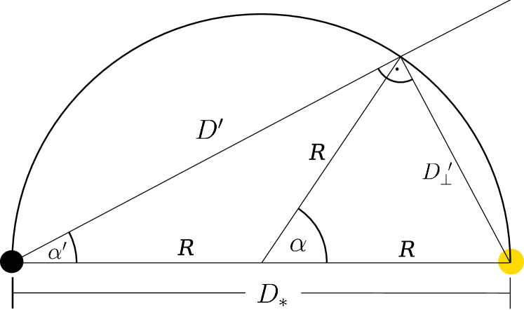
Figure 9: Geometry used for the calculation of the observed flux of re-scattered photons.

where the integration over the sphere $R=D_{*}/2$ incorporates all isotropically re-scattered components of the emission from the SMBH as seen by the observer. To account for the energy shift the integral has to be convolved with $P(\epsilon_{1}^{\prime}|\epsilon_{1})$. Integrating over $\phi$ and using the geometric relations $D^{\prime}=D_{*}\cos\alpha^{\prime}$ and $\alpha^{\prime}=\alpha/2$ reveals

$$\begin{split}f_{\nu}^{\rm casc}(\epsilon_{1}^{\prime})=&\frac{1}{2}\int d\epsilon_{1}P(\epsilon_{1}^{\prime}|\epsilon_{1})f_{\nu}(\epsilon_{1})\\ \times&\int\limits_{\alpha_{\mathrm{min}}}^{\alpha_{\mathrm{max}}}d\alpha^{\prime}\tan\alpha^{\prime}\left(1-\exp\left[-\tau(\alpha^{\prime},\epsilon_{1})\right]\right).\end{split}$$ (9)

The limit $\alpha_{\mathrm{min}}$ is given by the radius of the star while $\alpha_{\mathrm{max}}$ is defined by the $\gamma$-photosphere of the SMBH. The geometric effect results in a factor of $\approx 5\times 10^{-3}$ for VHE photons of energy $200\ {\rm GeV}$.

In order to evaluate the re-distribution kernel $P(\epsilon_{1}^{\prime}|\epsilon_{1})$, we use the differential pair-production cross section $d\sigma/d\gamma$ in the kinematically accessible range: $\epsilon_{1}(1-\sqrt{1-(\epsilon_{1}\epsilon_{2})^{-1})}<2\gamma<\epsilon_{1}(1+\sqrt{1-(\epsilon_{1}\epsilon_{2})^{-1})}$. This cross section is conveniently approximated (Agaronyan et al., 1983):

$$\begin{split}\frac{d\sigma}{d\gamma}(\epsilon_{1},\epsilon_{2},\gamma)=&\frac{3\sigma_{T}}{32\epsilon_{1}^{3}\epsilon_{2}^{2}}\left[\frac{4\epsilon_{1}^{2}}{\gamma(\epsilon_{1}-\gamma)}\ln\left(\frac{4\epsilon_{2}\gamma(\epsilon_{1}-\gamma)}{\epsilon_{1}}\right)-\right.\\ 8\epsilon_{1}\epsilon_{2}+&\left.\frac{2\epsilon_{1}^{2}(2\epsilon_{1}\epsilon_{2}-1)}{\gamma(\epsilon_{1}-\gamma)}-\left(1-\frac{1}{\epsilon_{1}\epsilon_{2}}\right)\frac{\epsilon_{1}^{4}}{\gamma^{2}(\epsilon_{1}-\gamma)^{2}}\right].\end{split}$$ (10)

This cross-section is accurate to the level of a few per cent in the limiting case of $\epsilon_{1}\gg\epsilon_{2}$ (see also discussion by Boettcher et al. (1997)). The assumption of isotropy underlying this approximation is not entirely justified. However, when evaluating the total cross section and the corresponding optical depth for the chosen geometry, the relative differences to the line of sight integration of the angle dependent cross section is a few per cent only. In order to evaluate $P$, the differential cross section is normalised such that

$$\begin{split}\frac{dn_{e}}{d\gamma}(\epsilon_{1},\epsilon_{2},\gamma)&=\frac{d\sigma}{d\gamma}(\epsilon_{1},\epsilon_{2},\gamma)\\ &\times\left(0.5\int d\epsilon\,n(\epsilon)\int d\gamma^{\prime}\frac{d\sigma}{d\gamma^{\prime}}(\epsilon_{1},\epsilon,\gamma^{\prime})\right)^{-1},\end{split}$$ (11)

taking into account that a pair of particles is produced. The inverse Compton scattering cross section has been taken from Blumenthal & Gould (1970)

$$\begin{split}\frac{d\sigma}{d\epsilon_{1}^{\prime}}(\epsilon_{1}^{\prime},\epsilon_{2},\gamma)&=\frac{3\sigma_{T}}{4\epsilon_{2}\gamma^{2}}\left[1+\frac{z^{2}}{2(1-z)}+\frac{z}{b(1-z)}-\right.\\ \frac{2z^{2}}{b^{2}(1-z)^{2}}&+\left.\frac{z^{3}}{2b(1-z)^{2}}-\frac{2z\ln(b(1-z)/z)}{b(1-z)}\right],\end{split}$$ (12)

with $z=\epsilon_{1}^{\prime}/\gamma$ and $b=4\epsilon_{2}\gamma$. Again, this differential cross section is normalised,

$$\begin{split}\frac{dn}{d\epsilon_{1}^{\prime}}(\epsilon_{1}^{\prime},\epsilon_{2},\gamma)&=\frac{d\sigma}{d\epsilon_{1}^{\prime}}(\epsilon_{1}^{\prime},\epsilon_{2},\gamma)\\ &\times\left(\int d\epsilon\,n(\epsilon)\int d\epsilon_{1}^{\prime}\frac{d\sigma}{d\epsilon_{1}^{\prime}}(\epsilon_{1}^{\prime},\epsilon,\gamma)\right)^{-1},\end{split}$$ (13)

so that finally

$$P(\epsilon_{1}^{\prime}|\epsilon_{1})=\int d\gamma\int d\epsilon\,n(\epsilon)\frac{dn}{d\epsilon_{1}^{\prime}}(\epsilon_{1}^{\prime},\epsilon,\gamma)\int d\epsilon^{\prime}\,n(\epsilon^{\prime})\frac{dn_{e}}{d\gamma}(\epsilon_{1},\epsilon^{\prime},\gamma).$$ (14)

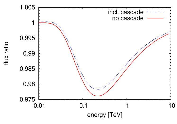
Figure 10: Flux ratio $f^{\mathrm{obs}}_{\nu}/f_{\nu}$ for the star S14 at the time of the largest absorption effect with (dashed blue) and without (solid red) the contribution of the photons from the cascade.

In Fig. 10 we display the effect of the cascade by showing the ratio of the observed flux to the initial flux with and without the additional cascade component. The result indicates a small increase of the flux when including the first generation cascade. The resulting change is similar to the uncertainties resulting from the uncertainties of the orbital elements. The slight bump due to the isotropic cascade radiation could in principle be observed even during the passage of a star far away from the line of sight (thus leading to no absorption effect). The effect is however at the level of 0.1 per cent and therefore not easily observable.

The additional feature (pile-up) in the energy spectrum at energies below the main absorption peak has a timing signature shifted with respect to the time-dependent absorption due to the cooling time of the electrons, which is in $\mathcal{O}(20)\ {\rm d}$. The resulting (time-dependent) emission spectrum of electrons cooling in the Klein-Nishina regime could in principle be calculated using the approach suggested by Manolakou et al. (2007). Given the smallness of the effect however, we consider it of little interest here.

Appendix B Parametrisation for the effective areas

For the effective areas $A_{\mathrm{eff}}(E)$ used in the simulation of the light-curves (Eq. 6) we used the following parametrisation:

$$A_{\mathrm{eff}}(E)=g_{1}\left(\frac{E}{\mathrm{MeV}}\right)^{-g_{2}}\exp\left(-\frac{g_{3}}{E}\right).$$ (15)

The parameters for the three different IACTs are given in Table 2. For H.E.S.S. and H.E.S.S. II the curve is based upon the effective area from Aharonian et al. (2006b) and Punch (2005) respectively. For CTA we assume the effective area to increase by a factor of 25 as given in Hermann et al. (2008).

Table 2: Parameters used for the calculation of the effective area for the three different IACTs.

	H.E.S.S.	H.E.S.S. II	CTA
$g_{1}$	$6.85\times 10^{9}\,\mathrm{cm}^{2}$	$2.05\times 10^{10}\,\mathrm{cm}^{2}$	$1.71\times 10^{11}\,\mathrm{cm}^{2}$
$g_{2}$	0.0891	0.0891	0.0891
$g_{3}$	$5\times 10^{5}\,\mathrm{MeV}$	$1\times 10^{5}\,\mathrm{MeV}$	$1\times 10^{5}\,\mathrm{MeV}$

References

- Acero et al. (2009) Acero F., et al., 2009, MNRAS, in press
- Agaronyan et al. (1983) Agaronyan F. A., Atoyan A. M., Nagapetyan A. M., 1983, Astrophysics, 19, 187
- Aharonian et al. (2004) Aharonian F., et al., 2004, A&A, 425, L13
- Aharonian et al. (2006a) Aharonian F., et al., 2006a, Physical Review Letters, 97, 221102
- Aharonian et al. (2006b) Aharonian F., et al., 2006b, A&A, 457, 899
- Aharonian et al. (2008) Aharonian F., et al., 2008, A&A, 492, L25
- Aharonian et al. (2009) Aharonian F., et al., 2009, A&A, 503, 817
- Aharonian & Neronov (2005) Aharonian F., Neronov A., 2005, ApJ, 619, 306
- Albert et al. (2006) Albert J., et al., 2006, ApJ, 638, L101
- Atoyan & Dermer (2004) Atoyan A., Dermer C. D., 2004, ApJ, 617, L123
- Balick & Brown (1974) Balick B., Brown R. L., 1974, ApJ, 194, 265
- Blumenthal & Gould (1970) Blumenthal G. R., Gould R. J., 1970, Reviews of Modern Physics, 42, 237
- Boettcher et al. (1997) Boettcher M., Mause H., Schlickeiser R., 1997, A&A, 324, 395
- Dubus (2006) Dubus G., 2006, A&A, 451, 9
- Eisenhauer et al. (2005) Eisenhauer F., Genzel R., Alexander T., Abuter R., Paumard T., 2005, ApJ, 628, 246
- Ghez et al. (2003) Ghez A. M., et al., 2003, ApJ, 586, L127
- Gillessen et al. (2009) Gillessen S., Eisenhauer F., Trippe S., Alexander T., Genzel R., Martins F., Ott T., 2009, ApJ, 692, 1075
- Gould & Schréder (1967) Gould R. J., Schréder G. P., 1967, Physical Review, 155, 1404
- Hermann et al. (2008) Hermann G., Hofmann W., Schweizer T., Teshima M., 2008, in Caballero R., et al. eds, Proc. 30th Int. Cosmic Ray Conf. Vol. 3, Cherenkov Telescope Array: The next-generation ground-based gamma-ray observatory. Mexico City, pp 1313–1316
- Hinton (2004) Hinton J. A., 2004, New Astronomy Review, 48, 331
- Horns (2005) Horns D., 2005, Physics Letters B, 607, 225
- Kosack et al. (2004) Kosack K., Badran H. M., Bond I. H., et al., 2004, ApJ, 608, L97
- Loeb (2004) Loeb A., 2004, MNRAS, 350, 725
- Maillard et al. (2004) Maillard J. P., Paumard T., Stolovy S. R., Rigaut F., 2004, A&A, 423, 155
- Manolakou et al. (2007) Manolakou K., Horns D., Kirk J. G., 2007, A&A, 474, 689
- Martins et al. (2008) Martins F., Gillessen S., Eisenhauer F., Genzel R., Ott T., Trippe S., 2008, ApJ, 672, L119
- Murray & Dermott (1999) Murray C. D., Dermott S. F., 1999, Solar System Dynamics. Cambridge University Press, Cambridge
- Punch (2005) Punch M., 2005, in Derange B., ed., Proc. Towards a network of Atmospheric Cherenkov Detectors VII p. 379
- Reid (2009) Reid M. J., 2009, International Journal of Modern Physics D, 18, 889
- Reid et al. (2007) Reid M. J., Menten K. M., Trippe S., Ott T., Genzel R., 2007, ApJ, 659, 378
- Schödel et al. (2002) Schödel R., et al., 2002, Nature, 419, 694
- Tsuchiya et al. (2004) Tsuchiya K., et al., 2004, ApJ, 606, L115
- Wang et al. (2006) Wang Q. D., Lu F. J., Gotthelf E. V., 2006, MNRAS, 367, 937