Features of ion acoustic waves in collisional plasmas

Abstract: The effects of friction on the ion acoustic (IA) wave in fully and partially ionized plasmas are studied. In a quasi-neutral electron-ion plasma the friction between the two species cancels out exactly and the wave propagates without any damping. If the Poisson equation is used instead of the quasi-neutrality, however, the IA wave is damped and the damping is dispersive. In a partially ionized plasma, the collisions with the neutrals modify the IA wave beyond recognition. For a low density of neutrals the mode is damped. Upon increasing the neutral density, the mode becomes first evanescent and then reappears for a still larger number of neutrals. A similar behavior is obtained by varying the mode wave-length. The explanation for this behavior is given. In an inhomogeneous plasma placed in an external magnetic field, and for magnetized electrons and un-magnetized ions, the IA mode propagates in any direction and in this case the collisions make it growing on the account of the energy stored in the density gradient. The growth rate is angle dependent. A comparison with the collision-less kinetic density gradient driven IA instability is also given.

PACS No: 52.35.Fp; 52.30.Ex

1 Introduction

Multi-component plasmas comprise different species that, in the presence of waves, may be in the state of relative macroscopic motion. In such a situation, friction between the species may lead to wave damping (though not always, as we are going to show in the forthcoming text). For example, neutrals in a weakly ionized plasma represent a barrier for electron and ion motion in a wave field. A similar friction appears in a fully ionized plasma when the electron and ion components do not share the same momentum. The interaction is described by a friction force $\vec{F}_{j}=m_{j}n_{j}\nu_{jl}(\vec{v}_{j}-\vec{v}_{l})$ in the momentum equation for the species $j$. Momentum conservation implies that for its counterpart $l$, $\vec{F}_{l}=m_{l}n_{l}\nu_{lj}(\vec{v}_{l}-\vec{v}_{j})$, where $m_{j}n_{j}\nu_{jl}=m_{l}n_{l}\nu_{lj}$. If the two species $j$ and $l$ have a large mass difference, the friction response of the heavier component is typically omitted as negligible in the literature. However, this may yield completely wrong results as we shall demonstrate in the forthcoming text using the ion acoustic (IA) mode as an example.

In the presence of high frequency waves $\omega\gg\Omega_{i}=eB_{0}/m_{i}$ in a plasma placed in an external magnetic field $\vec{B}_{0}=B_{0}\vec{e}_{z}$, ions will follow nearly straight lines regardless of the direction of the wave-number vector $\vec{k}$ and the magnetic field vector. For electrons, in view of the mass difference, the opposite may hold, $\omega\ll\Omega_{e}=eB_{0}/m_{e}$, hence they will behave as magnetized and their perpendicular and parallel dynamics will be essentially different [1]. Ions can behave as un-magnetized in the perturbed state also in case of collisions provided that $\nu_{i}>\Omega_{i}$ even if at the same time $\Omega_{i}>\omega$, or for short wavelengths $\lambda<\rho_{i}$, $\rho_{i}=v_{{\scriptscriptstyle T}i}/\Omega_{i}$, $v_{{\scriptscriptstyle T}i}^{2}=\kappa T_{i}/m_{i}$. In the case of an inhomogeneous equilibrium, with a density gradient perpendicular to the magnetic field vector, in the unperturbed state the ions may behave as un-magnetized in case of a low temperature, when their diamagnetic drift velocity becomes negligible as compared to electrons [for singly charged ions $v_{*i}/v_{*e}=T_{i}/T_{e}$, where $v_{*j}=\kappa T_{j}n_{j0}^{\prime}/(q_{j}B_{0}n_{j0})$, and $n_{j}^{\prime}=dn_{j}/dx$ denotes the equilibrium density gradient]. The same holds in the presence of numerous collisions as above, $\nu_{i}>\Omega_{i}$, when their diamagnetic effects are absent too.

In all these situations, and neglecting the electron polarization drift (inertia-less limit), the wave will still have the basic properties of the IA mode. Within the two-fluid theory such a mode in an inhomogeneous plasma [that may be called ion-acoustic-drift (IAD) mode] may in fact become growing [1]-[3] in the simultaneous presence of collisions and the mentioned equilibrium density gradient perpendicular to $\vec{B}_{0}$.

Within the kinetic theory the mode is also growing in the presence of the same density gradient and this even without collisions (due to purely kinetic effects), and the physics of the growth rate is similar to the standard drift wave instability [4]. It requires that the wave frequency is below the electron diamagnetic drift frequency $\omega_{*e}=v_{*e}k_{\bot}$.

On the other hand, keeping the electron inertia results in the instability of the lower-hybrid-drift (LHD) type [5]-[8]. In some other limits the effects of the same density gradient yield growing ion plasma (Langmuir) oscillations [5], or growing electron-acoustic oscillations [6].

In the present manuscript the friction force effects on the IA wave are discussed, both for fully and partially ionized un-magnetized plasmas, and for inhomogeneous plasmas with magnetized electrons. The latter implies growing modes within both the fluid and kinetic descriptions, and in the manuscript these two instabilities are compared.

2 IA wave in fully and partially ionized collisional plasmas

The equations used further in this section are the momentum equations for the ions, the electrons and the neutral particles, respectively:

$$m_{i}n_{i}\left(\frac{\partial}{\partial t}+\vec{v}_{i}\cdot\nabla\right)\vec{v}_{i}=-en_{i}\nabla\phi-\kappa T_{i}\nabla n_{i}-m_{i}n_{i}\nu_{ie}(\vec{v}_{i}-\vec{v}_{e})-m_{i}n_{i}\nu_{in}(\vec{v}_{i}-\vec{v}_{n}),$$ (1)

$$m_{e}n_{e}\left(\frac{\partial}{\partial t}+\vec{v}_{e}\cdot\nabla\right)\vec{v}_{e}=en_{e}\nabla\phi-\kappa T_{e}\nabla n_{e}-m_{e}n_{e}\nu_{ei}(\vec{v}_{e}-\vec{v}_{i})-m_{e}n_{e}\nu_{en}(\vec{v}_{e}-\vec{v}_{n}),$$ (2)

and

$$m_{n}n_{n}\left(\frac{\partial}{\partial t}+\vec{v}_{n}\cdot\nabla\right)\vec{v}_{n}=-\kappa T_{n}\nabla n_{n}-m_{n}n_{n}\nu_{ni}(\vec{v}_{n}-\vec{v}_{i})-m_{n}n_{n}\nu_{ne}(\vec{v}_{n}-\vec{v}_{e}),$$ (3)

and the continuity equation

$$\frac{\partial n_{j}}{\partial t}+\nabla\cdot(n_{j}\vec{v}_{j})=0,\quad{j=e,i,n}.$$ (4)

This set of equations is closed either by using the quasi-neutrality or the Poisson equation. The differences between the two cases are discussed below.

2.1 Friction in electron-ion plasma

The continuity equation (4) yields

$$v_{i1}=\omega n_{i1}/(kn_{0}),\quad v_{e1}=\omega n_{e1}/(kn_{0}),$$ (5)

so that the velocity difference in the friction term $v_{e}-v_{i}\equiv 0$ if the quasi-neutrality is used. The IA mode propagates without any damping. Hence, the friction force in a fully ionized plasma in this limit cancels out exactly even without using the momentum balance. The physical reason for this is the assumed exact balance of the perturbed densities: what one plasma component loses the other component receives, this is valid at every position in the wave and no momentum is lost.

A typical mistake seen in the literature is to take the friction force term for electrons only, in the form $m_{e}n_{e}\nu_{ei}\vec{v}_{e}$. This comes with the excuse of the large mass difference, so that the displacement of the much heavier ion fluid, caused by the electron friction is neglected. In the case of a fully ionized electron-ion plasma this yields a false damping of the IA mode within the quasi-neutrality limit:

$$\omega=\pm k(c_{s}^{2}+v_{{\scriptscriptstyle T}i}^{2})^{1/2}-\nu_{ei}/2.$$ (6)

On the other hand, if the Poisson equation is used instead of the quasi-neutrality, one obtains [9]

$$\omega=\pm kv_{s}\left(1-r_{de}^{2}k^{2}\frac{\nu_{ie}^{2}r_{de}^{2}}{v_{s}^{2}}\right)^{1/2}-i\nu_{ie}r_{de}^{2}k^{2}.$$ (7)

Here, we have used the momentum conservation $\nu_{ie}=m_{e}\nu_{ei}/m_{i}$ and $v_{s}^{2}=c_{s}^{2}+v_{{\scriptscriptstyle T}i}^{2}$, $r_{de}=v_{{\scriptscriptstyle T}e}/\omega_{pe}$. The physical reason for damping in the present case is the fact that the detailed balance $n_{i1}=n_{e1}$ does not hold, because of the electric field which takes part for small enough wave-lengths. It can easily be seen that for any realistic parameters the second term in the real part of the frequency in Eq. (7) is much below unity and the mode is never evanescent. However, in partially ionized plasmas (see below) this may be completely different.

2.2 Friction and collisions in partially ionized plasma

Keeping the quasi-neutrality limit, we now discuss the IA wave damping in plasmas comprising neutrals as well. In view of the results presented above, the electron-ion friction terms in Eqs. (1) and (2) will cancel each other out and in a few steps one derives the following dispersion equation containing the collisions of plasma species with neutrals and vice versa:

$$\omega^{3}+i\omega^{2}\left(\nu_{en}\frac{m_{e}}{m_{i}}+\nu_{in}\right)\left(1+\frac{m_{i}}{m_{n}}\frac{n_{0}}{n_{n0}}\right)-k^{2}c_{s}^{2}\,\omega$$

$$-ik^{2}c_{s}^{2}\,\frac{m_{e}}{m_{n}}\frac{n_{0}}{n_{n0}}\left(\nu_{en}+\frac{m_{i}}{m_{e}}\nu_{in}\right)=0.$$ (8)

In the derivation, the ion and neutral thermal terms are neglected. The ion thermal terms would give the modified mode frequency $\omega^{2}=k^{2}c_{s}^{2}(1+T_{i}/T_{e})$. Hence, even if $T_{e}=T_{i}$ the wave frequency is only modified by a factor $2^{1/2}$. The neutral thermal terms are discussed further in the text.

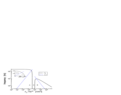
Figure 1: Frequency $\omega_{r}$ and absolute value of the IA mode damping $|\gamma|$ in terms of the number density of neutrals. Details of the mode behavior in the region A are better seen in the linear scale (small figure inside).

Note that in deriving Eq. (8), the momentum conservation condition $\nu_{ie}=m_{e}\nu_{ei}/m_{i}$ is nowhere used: the e-i and i-e friction terms exactly vanish in view of Eq. (5).

Equation (8) is solved numerically for a plasma containing electrons, protons, and neutral hydrogen atoms using the following set of parameters: $T_{e}=4\;$eV, $n_{0}=10^{18}\;$m^-3, $k=10\;$m^-1, with [10] $\sigma_{en}=1.14\cdot 10^{-19}\;$m^-2. The neutral density is varying in the interval $10^{16}-10^{23}\;$m^-3. The ion and hydrogen temperatures are taken $T_{i}=T_{n}=T_{e}/20$, satisfying the condition of their small thermal effects. This also gives [11], $\sigma_{in}=2.24\cdot 10^{-18}\;$m^-2. The results are presented in Fig. 1. The IA mode propagates in two distinct regions A and B.

Only a limited left part of the region A would correspond to the ’standard’ IA wave behavior in a collisional plasma: the mode is damped and the damping is proportional to the neutral number density. Hence, in this region it may be more or less appropriate to use the approximate expressions for the friction force, like (in the case of electrons) $F_{e}\simeq m_{e}n_{0}\nu_{en}v_{e1}$. However, this domain is very limited because in the rest of the domain the frequency drops and the mode becomes non-propagating for $n_{n0}\geq 3.8\cdot 10^{19}\;$m^-3 (this is the lower limit of the region C in Fig. 1).

Increasing the neutral number density, after some critical value (in the present case this is around $n_{n0}\simeq 10^{20}\;$m^-3) the IA mode reappears again in the region B, with a frequency starting from zero. For even larger neutrals number densities, the mode damping in fact vanishes completely and the wave propagates freely but with a frequency that is many orders of magnitude below the ideal case $kc_{s}\simeq 196\;$kHz. This behavior can be explained in the following manner. For a relatively small number of collisions the IA mode is weakly damped because initially neutrals do not participate in the wave motion and do not share the same momentum. Increasing the number of neutrals, the damping may become so strong that the wave becomes evanescent. However, for much larger collision frequencies (i.e., for a lower ionization ratio), the tiny population of electrons and ions is still capable of dragging neutrals along and all three components move together. The plasma and the neutrals become so strongly coupled that the two essentially different fluids participate in the electrostatic wave together. In this regime, the stronger the collisions are, the less wave damping there is! Yet, this a bit counter-intuitive behavior comes with a price: the wave frequency and the wave energy flux becomes reduced by several orders of magnitude.

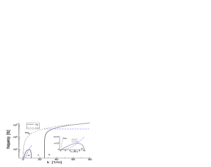
Figure 2: Frequency $\omega_{r}$ and absolute value of the IA mode damping $|\gamma|$ in terms of the wave number. The line $kc_{s}$ shows part of the graph of the ideal mode. Details of the domain $a$ are better seen in the linear scale (small figure inside).

Similar effects may be expected by varying the wave-length. The previous role of the varying density of neutrals is now replaced by the the ratio of the mean free path of a species $\lambda_{fj}=v_{{\scriptscriptstyle T}j}/\nu_{j}$ (with respect to their collision with neutrals) and the wavelength. This ratio now determines the coupling between the plasma and the neutrals. The mode behavior is directly numerically checked by fixing $n_{n0}=10^{20}\;$m^-3, $n_{0}=10^{18}\;$m^-3, and for other parameters same as above. For these parameters we have $\lambda_{fe}=v_{{\scriptscriptstyle T}e}/\nu_{en}=0.09$ m, and $\lambda_{fi}=v_{{\scriptscriptstyle T}i}/\nu_{in}=0.004$. The numerical results are presented in Fig. 2 for $k$ varying in the interval $0.2-80\;$m^-1. The mode vanishes in the interval $c$, between $k\simeq 10\;$m^-1 and $k\simeq 25.6\;$m^-1. The explanation is similar as before. Note that for $k=0.2\;$m^-1 (in the region $a$) we have $\omega_{r}\simeq 390\;$Hz, and this is about one order below $kc_{s}$. Compared to the mode behavior in Fig. 1, this implies that the mode in the present domain $a$ is in the regime equivalent to the domain B from Fig. 1; here, in Fig. 2, these large wave-lengths imply well coupled plasma-neutrals, where the frequency is reduced and the damping is small. The region $a$ is also given separately in linear scale together with the dotted line describing the ideal mode $kc_{s}$. Clearly, in general the realistic behavior of the wave is beyond recognition and completely different as compared to the ideal case.

Figure 3: The two lines give the lower and upper values of the neutrals’ density $n_{n0}$ between which, for the given plasma density $n_{0}$, the IA mode does not propagate.

After checking for various sets of plasma densities, it appears that the evanescence region reduces and vanishes for larger plasma densities $n_{0}$. This is presented in Fig. 3 for the same parameters as above, by taking $k=10\;$m^-1, but for a varying plasma density $n_{0}$. The two lines represent boundary values of the number densities of neutrals, for the given plasma density, at which the IA mode vanishes; for the neutrals densities between the two lines the IA mode does not propagate. The symbols $*$ on the two lines denote the boundaries of the region $C$ from Fig. 1. It is seen that for the given case the IA mode propagates without evanescence for the plasma densities above $n_{0}=3.8\cdot 10^{18}\;$m^-3. Physical reason for a larger non-propagating domain for low plasma density is obvious, namely the tiny plasma population is less efficient in inducing a synchronous motion of neutrals. In the other limit, the opposite happens and the forbidden region eventually vanishes.

Figure 4: Values of the wave-number, in terms of the plasma density, for which the IA wave becomes evanescent. In the region between the lines the mode does not propagate.

A similar check is done by varying the wave-number and the plasma density, and the result is presented in Fig. 4 for a fixed $n_{n0}=10^{20}\;$m^-3. The lines represent the values $(n_{0},k)$ at which the IA wave becomes evanescent. There can be no wave in the region between the lines. On the other hand, there is no evanescence for the plasma density above $n_{0}=1.2\cdot 10^{19}\;$m^-3. Here $*$ denote the boundaries of the region $c$ from Fig. 2.

All these results clearly indicate that in practical measurements in laboratory and space plasmas, the IA mode can hardly be detected and recognized as the IA mode unless collisions are correctly taken into account (using full friction terms), and the mode is sought in the corresponding domain which follows from our Eq. (8).

2.3 Thermal effects of neutrals

Keeping the pressure terms for ions and neutrals yields the following dispersion equation

$$\omega^{4}+i\omega^{3}\left(\nu_{in}+\nu_{en}\frac{m_{e}}{m_{i}}\right)\left(1+\frac{m_{i}}{m_{n}}\frac{n_{0}}{n_{n0}}\right)-k^{2}\left(v_{s}^{2}+v_{{\scriptscriptstyle T}n}^{2}\right)\omega^{2}$$

$$-i\omega k^{2}\left[\frac{n_{0}}{n_{n0}}\frac{m_{i}}{m_{n}}v_{s}^{2}\left(\nu_{in}+\nu_{en}\frac{m_{e}}{m_{i}}\right)+\nu_{in}v_{{\scriptscriptstyle T}n}^{2}\right]+k^{4}v_{{\scriptscriptstyle T}n}^{2}v_{s}^{2}=0.$$ (9)

Here, $v_{s}^{2}=c_{s}^{2}+v_{{\scriptscriptstyle T}i}^{2}$. Without collisions, this yields two independent modes, viz. the ion-acoustic mode and the gas thermal (GT) mode, $(\omega^{2}-k^{2}v_{{\scriptscriptstyle T}n}^{2})(\omega^{2}-k^{2}v_{s}^{2})=0$. The collisions couple the two modes, and in order to compare with the previous cases we solve Eq. (9) for $k=10\;$m^-1, $n_{0}=10^{18}\;$m^-3, $T_{e}=4\;$eV, $T_{i}=T_{e}/20$, and in terms of the density and temperature of neutrals. For a low thermal contribution of neutrals (i.e., a low neutral temperature, or/and heavy neutral atoms) the previous results remain valid. Larger values of $v_{{\scriptscriptstyle T}n}$ introduce new effects, this is checked by varying the temperature $T_{n}$. The ion thermal terms do not make much difference, as explained earlier. The real part of the frequency $\omega_{g}$ of the gas thermal mode is presented in Fig. 5, and this only in a limited region that includes the evanescence area $C$ from Fig. 1. The damping is not presented but the mode is in fact heavily damped.

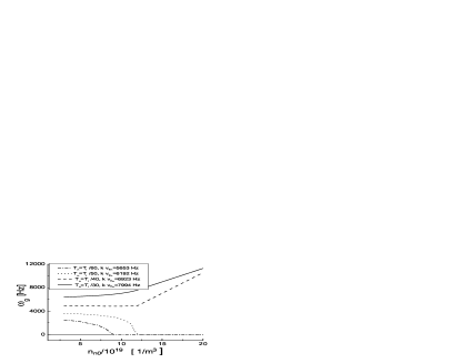
Figure 5: The real part of the frequency of damped gas thermal mode in terms of the number density of neutrals and for several temperatures of the neutrals gas.

The explanation of the figure is as follows. The starting solution for $T_{n}=0$ is in fact the line $\omega_{g}=0$, and this case would correspond to the the IA mode from Fig. 1. For some finite $T_{n}$ there appears the GT mode. For a low gas temperature the mode becomes evanescent for a higher density of neutrals (the dot and dash-dot lines in Fig. 5). This evanescence is accompanied with the previously discussed evanescence and re-appearance of the IA mode (described earlier and no need to be presented here again). However, for still larger $T_{n}$, the IA and GT modes become indistinguishable and propagate as one single mode. This is presented by the two upper (the full and dashed) lines in Fig. 5, that go up for large enough $n_{n0}$. Also given are the corresponding ideal values $kv_{{\scriptscriptstyle T}n}$ that appear to be much above the actual wave frequency $\omega_{g}$ in such a collisional plasma, but this remains so only until the neutral density $n_{n0}$ exceeds some critical value. After that the wave in fact behaves as less and less collisional and the wave frequency is increased.

3 IA wave instability in inhomogeneous partially ionized plasma

3.1 Fluid description in collisional plasma

In the previous text, collisions were shown to yield damping of the IA mode. However, if the plasma is inhomogeneous, implying the presence of source of free energy in the system, a drift-type instability of the IA wave may develop if there is a magnetic field $\vec{B}_{0}=B_{0}\vec{e}_{z}$ present, and the electrons (ions) are magnetized (un-magnetized). The magnetic field introduces a difference in the parallel and perpendicular dynamics of the magnetized species so that the continuity condition in this case can be written as

$$\frac{\partial n_{j1}}{\partial t}+n_{j0}\nabla\cdot\vec{v}_{j1}+\vec{v}_{j1}\cdot\nabla n_{j0}=0.$$ (10)

Here, $\nabla\equiv\nabla_{\bot}+\nabla_{z}$. For the un-magnetized species the direction of the wave plays no role so that $\nabla\rightarrow i\vec{k}$, $k^{2}=k_{y}^{2}+k_{z}^{2}$. On the other hand, for the equilibrium gradient along the $x$-axis and for perturbations of the form $\sim f(x)\exp(-i\omega t+ik_{y}y+ik_{z}z)$, where $|(df/dx)/f|,|(dn_{j0}/dx)/n_{0}|\ll k_{y}$, we apply a local approximation, and for ions the last term in Eq. (10) vanishes because of the assumed geometry. The ions’ dynamics is basically the same as in the previous sections.

The electron momentum equation (2) will now include the Lorentz force term $-en_{e}\vec{v}_{e}\times\vec{B}$. Repeating the derivation from Ref. [3], the total perpendicular electron velocity can be written as

$$v_{e\bot}=\frac{1}{1+\nu_{en}^{2}\alpha^{2}/\Omega_{e}^{2}}\left[\frac{1}{B_{0}}\vec{e}_{z}\times\nabla_{\bot}\phi+\frac{\nu_{en}\alpha}{\Omega_{e}}\frac{\nabla_{\bot}\phi}{B_{0}}-\frac{v_{\scriptscriptstyle{T}e}^{2}\nu_{en}\alpha}{\Omega_{e}^{2}}\frac{\nabla_{\bot}n_{e}}{n_{e}}-\frac{v_{\scriptscriptstyle{T}e}^{2}}{\Omega_{e}}\vec{e}_{z}\times\frac{\nabla_{\bot}n_{e}}{n_{e}}\right].$$ (11)

In the direction along the magnetic field vector, the perturbed electron velocity is

$$v_{ez1}=\frac{ik_{z}v_{{\scriptscriptstyle T}e}^{2}}{\nu_{en}}\frac{\omega^{2}+\nu_{ne}^{2}}{\omega^{2}-i\nu_{ne}\omega}\left(\frac{e\phi_{1}}{\kappa T_{e}}-\frac{n_{e1}}{n_{0}}\right).$$ (12)

Here, $\alpha=\omega/(\omega+i\nu_{ne})$, and for magnetized electrons, $|\nu_{en}^{2}\alpha^{2}/\Omega_{e}^{2}|\ll 1$ in the denominator in Eq. (11). Using these equations in the continuity condition (10) for electrons one obtains

$$\frac{n_{e1}}{n_{0}}=\frac{\omega_{*e}+iD_{p}+iD_{z}(\omega^{2}+\nu_{ne}^{2})/(\omega^{2}-i\nu_{ne}\omega)}{\omega+iD_{p}+iD_{z}(\omega^{2}+\nu_{ne}^{2})/(\omega^{2}-i\nu_{ne}\omega)}\frac{e\phi_{1}}{\kappa T_{e}},$$ (13)

$$D_{p}=\nu_{en}\alpha k_{y}^{2}\rho_{e}^{2},\quad D_{z}=k_{z}^{2}v_{{\scriptscriptstyle T}e}^{2}/\nu_{en},\quad\rho_{e}=v_{{\scriptscriptstyle T}e}/\Omega_{e}.$$

The term $D_{p}$ describes the effects of collisions on the electron perpendicular dynamics and is usually omitted in the literature. However, as shown in a recent study [3], it can strongly modify the growth rate of the drift and IA-drift wave instability in the limit of small parallel wave-number $k_{z}$.

Neglecting the neutral dynamics is equivalent to setting $\nu_{ne}=0$. This yields $\alpha=1$, and Eq. (13) becomes identical to the corresponding expression in Refs. [2, 12]. For a negligible $D_{p}$, Eq. (13) becomes the same as the corresponding equation from Ref. [13]. For negligible ion thermal effects, the final dispersion equation reads

$$\frac{k^{2}c_{s}^{2}}{\omega^{2}}=\frac{\omega_{*e}+iD_{p}+iD_{z}(\omega^{2}+\nu_{ne}^{2})/(\omega^{2}-i\nu_{ne}\omega)}{\omega+iD_{p}+iD_{z}(\omega^{2}+\nu_{ne}^{2})/(\omega^{2}-i\nu_{ne}\omega)}.$$ (14)

Equation (14) can be solved numerically keeping in mind a number of conditions used in their derivations, like smallness of the plasma beta to remain in electrostatic limit, smallness of the parallel phase velocity as compared to the electron thermal speed because of the massless electrons limit, also the ratio $D_{p}/D_{z}$ should be kept not too big or too small in order to have the assumed effects of electron collisions in perpendicular direction. We plan to compare this collisional instability with the kinetic instability due to the presence of the density gradient. Therefore, the wave frequency should be below the electron diamagnetic frequency etc.

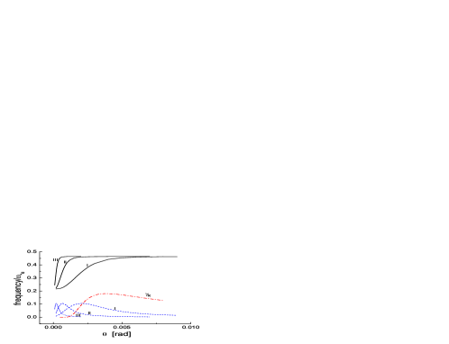
Figure 6: Real part of the frequency from Eq. (14) (full lines) and the corresponding growth rates (dashed lines), both normalized to the electron diamagnetic drift frequency, for three values of neutral number density. The lines I, II, III correspond (respectively) to $n_{n0}=10^{19},\,10^{18},\,10^{17}\;$m^-3. The line $\gamma_{k}$ is the kinetic growth-rate from Eq. (19) (for the same parameters as line II).

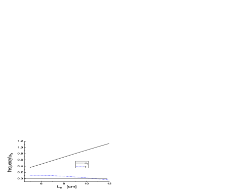
Figure 7: The real and imaginary parts of the frequency for the line II from Fig. 6, in terms of the characteristic density inhomogeneity scale length $L_{n}=(dn_{0}/dx)^{-1}$, and for the angle $\theta$ at the maximum on Fig. 6.

We solve Eq. (14) for an electron-argon plasma in the presence of parental argon atoms. As an example we take $T_{e}=4\;$eV, $T_{i}=T_{n}=T_{e}/30$, $n_{0}=10^{15}\;$m^-3, $B_{0}=1.2\cdot 10^{-2}\;$T, $k=500\;$m^-1, $L_{n}=0.05\;$m, and take several values for the density of neutrals. The result in terms of the angle of the propagation $\theta=\arctan(k_{z}/k_{y})$ is presented in Fig. 5. The three lines (full for the real part of the frequency, and dashed for the growth rates) are for $n_{n0}=10^{19},\,10^{18},\,10^{17}\;$m^-3. It is seen that i) the instability is angle dependent and there exists an angle of preference and an instability window in terms of $\theta$ within which the mode is most easily excited, ii) this angle of preference is shifted towards smaller values for lower values of the neutral density, and iii) in the same time the instability window becomes considerably reduced. This shows an interesting possibility of launching the IA-drift wave in a certain direction by simply varying the pressure of the neutral gas.

Varying the density scale length $L_{n}=(dn_{0}/dx)^{-1}$ the wave frequency may become above $\omega_{*e}$ and in this case the instability vanishes. As an example, this is demonstrated in Fig. 7 for the parameters corresponding to the line II from Fig. 6 and for the angle $\theta$ at the maximum growth rate. The growth rate changes the sign for $\omega\simeq\omega_{*e}$.

3.2 Comparison with collision-less kinetic gradient-driven IA wave instability

Keeping the same model of magnetized (un-magnetized) electrons (ions), within the kinetic theory the perturbed number density for electrons can be written as [14]

$$\frac{n_{e1}}{n_{0}}=\frac{e\phi_{1}}{\kappa T_{e}}\left\{1+i\left(\frac{\pi}{2}\right)^{1/2}\frac{\omega-\omega_{*e}}{k_{z}v_{{\scriptscriptstyle T}e}}\exp\left[-\omega^{2}/(2k_{z}^{2}v_{{\scriptscriptstyle T}e}^{2})\right]\right\}.$$ (15)

In the derivation of Eq. (15) the electron Larmor radius corrections are neglected in terms of the type $I_{n}(b)\exp(-b)$, $b=k_{\bot}^{2}\rho_{e}^{2}$, where $I_{n}$ denotes the modified Bessel function of the first kind, order $n$, and only $n=0$ terms are kept for the present case of frequencies much below the gyro-frequency.

The ion number density can be calculated using the kinetic description for un-magnetized species, the derivation is straight-forward and it yields [15]

$$\frac{n_{i1}}{n_{i0}}=-\frac{e\phi_{1}}{m_{i}v_{{\scriptscriptstyle T}i}^{2}}\left[1-J_{+}\left(\frac{\omega_{i}}{kv_{{\scriptscriptstyle T}i}}\right)\right].$$ (16)

Here, $J(\eta)=[\eta/(2\pi)^{1/2}]\int_{c}d\zeta\exp(-\zeta^{2}/2)/(\eta-\zeta)$ is the plasma dispersion function, and $\zeta=v/v_{{\scriptscriptstyle T}i}$. In the case $|\eta|\gg 1$, and assuming $|Re(\eta)|\gg Im(\eta)$, an expansion is used for $J(\eta)$. This together with the quasi-neutrality yields the kinetic dispersion equation for the IA-drift wave:

$$\Delta(\omega,k)\equiv 1-\frac{k^{2}c_{s}^{2}}{\omega^{2}}-\frac{3k^{4}v_{{\scriptscriptstyle T}i}^{2}c_{s}^{2}}{\omega^{4}}$$

$$+i(\pi/2)^{1/2}\left\{\frac{\omega-\omega_{*e}}{k_{z}v_{{\scriptscriptstyle T}e}}\exp\left[-\omega^{2}/(2k_{z}^{2}v_{{\scriptscriptstyle T}e}^{2})\right]+\frac{T_{e}}{T_{i}}\frac{\omega}{kv_{{\scriptscriptstyle T}i}}\exp\left[-\omega^{2}/(2k^{2}v_{{\scriptscriptstyle T}i}^{2})\right]\right\}.$$ (17)

The real part of Eq. (17) yields the spectrum

$$\omega_{k}^{2}=\frac{k^{2}c_{s}^{2}}{2}\left[1+\left(1+12T_{i}/T_{e}\right)^{1/2}\right].$$ (18)

The kinetic growth rate is given by

$$\gamma_{k}\simeq-Im\Delta/(\partial Re\Delta/\partial\omega)=-\frac{(\pi/2)^{1/2}\omega_{k}^{3}}{2k^{2}c_{s}^{2}}\times$$

$$\times\left\{\frac{\omega_{k}-\omega_{*e}}{k_{z}v_{{\scriptscriptstyle T}e}}\exp\left[-\omega_{k}^{2}/(2k_{z}^{2}v_{{\scriptscriptstyle T}e}^{2})\right]+\frac{T_{e}}{T_{i}}\frac{\omega_{k}}{kv_{{\scriptscriptstyle T}i}}\exp\left[-\omega_{k}^{2}/(2k^{2}v_{{\scriptscriptstyle T}i}^{2})\right]\right\}.$$ (19)

Here, the index $k$ is used to denote kinetic expressions. The electron contribution in Eq. (19) yields a kinetic instability provided that $\omega_{k}<\omega_{*e}$.

Equation (19) is solved numerically and compared with the growth rate obtained from the collisional IA-drift mode (8). For a fixed $k=500\;$m^-1 as in Figs. 6 and 7, the normalized frequency $\omega_{k}/\omega_{*e}=0.485$, and the result for the growth rate is presented by the line $\gamma_{k}$ in Fig. 6 for the parameters corresponding to the line II from the fluid analysis (i.e., for $n_{n0}=10^{18}\;$m^-3). The larger kinetic growth rate appears also to be angle dependent, yet with a much wider instability window as compared to the collisional gradient driven instability obtained from the fluid theory.

4 Summary

The analysis of the ion acoustic wave presented here shows the importance of collisions in describing the wave behavior. Without a proper analytical description, the identification of the mode in the laboratory and space observations may be rather difficult because one might fruitlessly search for the wave in a very inappropriate domain, as can be concluded from the graphs presented here, and in particular from Fig. 2. Not only the wave frequency may become orders of magnitude below an expected ideal value, but also the mode may completely vanish. A similar analysis of the effects of collisions may be performed for other plasma modes as well, like the Alfvén wave etc, as predicted long ago in classic Ref. [16]. The impression is that these effects are frequently overlooked in the literature, hence the necessity for the quantitative analysis given in the present work that can be used as a good starting point for an eventual experimental check of the wave behavior in collisional plasmas. Particularly interesting for experimental investigations may be the angle dependent mode behavior given in Sec. 3, where it is shown that the strongly growing mode may be expected within a given narrow instability window in terms of the angle of propagation. Comparison with the kinetic theory shows a less pronounced angle dependent peak, yet this kinetic effect can effectively be smeared out in the presence of numerous collisions, that are known to reduce kinetic effects in any case, and the sharp angle dependence that follow from pure fluid effects should become experimentally detectable.

Acknowledgements:

The results presented here are obtained in the framework of the projects G.0304.07 (FWO-Vlaanderen), C 90347 (Prodex), GOA/2009-009 (K.U.Leuven). Financial support by the European Commission through the SOLAIRE Network (MTRN-CT-2006-035484) is gratefully acknowledged.

References

- [1] N. A. Krall, in Advances in Plasma Physics, ed. A Simon and W. B. Thompson (Interscience, New York, 1968), vol. 1, p. 195.
- [2] A. B. Mikhailovskii, Theory of Plasma Instabilities (Consultants Bureau, New York, 1974), vol. 2, p. 192.
- [3] J. Vranjes and S. Poedts, Phys. Plasmas 16, 022101 (2009).
- [4] N. A. Krall and D. Book, Phys. Rev. Lett. 23, 574 (1969); ibid., Phys. Fluids 12, 347 (1969).
- [5] N. A. Krall and P. C. Liewer, Phys. Rev. A 4, 2094 (1971).
- [6] M. Mohan and M. Y. Yu, J. Plasma Phys. 29, 127 (1983).
- [7] M. Bose and S. Guha, Phys. Scripta 34, 63 (1986).
- [8] J. D. Huba, A. B. Hassam, and D. Winske, Phys. Fluids B 2, 1676 (1990).
- [9] J. Vranjes, M. Kono, S. Poedts, and M. Y. Tanaka, Phys. Plasmas 15, 092107 (2008).
- [10] B. Bedersen and L. J. Kiefer, Rev. Mod. Phys. 43, 601 (1971).
- [11] P. S. Krstic and D. R. Schultz, J. Phys. B: Mol. Opt. Phys. 32, 3485 (1999).
- [12] J. Vranjes, D. Petrovic, B. P. pandey, and S. Poedts, Phys. Plasmas 15, 072104 (2008).
- [13] J. Vranjes and S. Poedts, Phys. Plasmas 15, 034504 (2008).
- [14] J. Weiland, Collective Modes in Inhomogeneous Plasmas (Institute of Physics Pub., Bristol, 2000) p. 59.
- [15] J. Vranjes and S. Poedts, Eur. Phys. J. D 40, 257 (2006).
- [16] B. S. Tanenbaum and D. Mintzer, Phys. Fluids 5, 1226 (1962).