Effective low-energy Hamiltonians for interacting nanostructures

Abstract

We present a functional renormalization group (fRG) treatment of trigonal graphene nanodiscs and composites thereof, modeled by finite-size Hubbard-like Hamiltonians with honeycomb lattice structure. At half filling, the noninteracting spectrum of these structures contains a certain number of half-filled states at the Fermi level. For the case of trigonal nanodiscs, including interactions between these degenerate states was argued to lead to a large ground state spin with potential spintronics applications Ezawa (2009). Here we perform a systematic fRG flow where the excited single-particle states are integrated out with a decreasing energy cutoff, yielding a renormalized low-energy Hamiltonian for the zero-energy states that includes effects of the excited levels. The numerical implementation corroborates the results obtained with a simpler Hartree-Fock treatment of the interaction effects within the zero-energy states only. In particular, for trigonal nanodiscs the degeneracy of the one-particle-states with zero-energy turns out to be very robust against influences of the higher levels. As an explanation, we give a general argument that within this fRG scheme the zero-energy degeneracy remains unsplit under quite general conditions and for any size of the trigonal nanodisc. We furthermore discuss the differences in the effective Hamiltonian and their ground states of single nanodiscs and composite bow-tie-shaped systems.

I Introduction

Graphene-nanodiscs (GNDs) are nanostructures consisting of a finite bipartite honeycomb-lattice. Among them a large variety of shapes is possible. Of particular interest are GNDs with a large ground state degeneracy where interaction effects can lead to the formation of a high spin state with relatively long lifetime that could be used in spintronics applications Ezawa (2009); Fernández-Rossier and Palacios (2007); Wang et al. (2009). In a tight-binding-description metallic GNDs with half-filled zero-energy-states are very rare Ezawa (2007). As shown in Fajtlowicz et al. (2005) the emergence of zero-energy-states is related to the morphology of the honeycomb-lattice. The number of these states $\eta$ is equal to the difference $\eta=\alpha-\beta$, where $\alpha$ and $\beta$ are the maximum numbers of nonadjacent vertices and edges. Following a classification in Ref. Wang et al. (2008) we distinguish between GNDs where $\eta$ is equal to the sublattice-imbalance $|L_{B}-L_{A}|$ of the bipartite honeycomb-lattice consisting of the two sublattices A and B and GNDs where $\eta>|L_{B}-L_{A}|$. $L_{A}$ and $L_{B}$ are the numbers of lattice sites on sublattice A and B.

One example for the first class are trigonal zigzag-GNDs (cf. Fig. 1.a) which are characterised by the size-parameter $N$. The sublattice-imbalance is $N=L_{B}-L_{A}$ and $\eta$ is equal to $N$. In contrast, bow-tie-shaped nanostructures (cf. Fig. 1.b) represent the second class with zero sublattice-mismatch but with $\eta>0$.

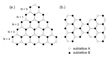
Figure 1: Two different kinds of graphene-nanodiscs: (a.) Trigonal zigzag-nanodiscs, that can be characterized by the size-parameter $N$. Here the zero-energy-degeneracy $\eta$ is equal to the sublattice-imbalance $L_{B}-L_{A}=N$ (b.) bow-tie-shaped nanostructure with zero sublattice mismatch and $\eta=2$.

To describe electron-electron-interactions in graphene nanodiscs it is common to take a $p_{z}$-band Hubbard-like model of the form

$$\hat{H}=-t\sum_{\langle i,j\rangle,\sigma}c^{{\dagger}}_{i,\sigma}c_{j,\sigma}+U\sum_{i}\hat{n}_{i,\uparrow}\hat{n}_{i,\downarrow}+\frac{V_{1}}{2}\sum_{\langle i,j\rangle,\sigma,\sigma^{\prime}}\hat{n}_{i,\sigma}\hat{n}_{j,\sigma^{\prime}}$$ (1)

where the sum goes over all nearest neighboring sites $\langle i,j\rangle$. The operators $c_{i,\sigma}^{{\dagger}}$ and $c_{i,\sigma}$ create and annihilate electrons with spin $\sigma$ on site $i$. The nearest-neighbor hopping-amplitude $t$ is of the order of 3$eV$.

For nearest-neighbor interaction $V_{1}=0$ an exact theorem by Lieb Lieb (1989) exists stating that the ground state spin of a repulsive Hubbard model on a bipartite lattice with sublattice site numbers $L_{A}$ and $L_{B}$ and $L_{A}+L_{B}$ even is equal to $S=\frac{1}{2}|L_{B}-L_{A}|$. From this it can be expected that the electron-spins of trigonal zigzag-GNDs prefer ferromagnetic order, while in bow-tie-shaped structures they adopt a total-spin-zero state. Of course, this argument is restricted to onsite interactions, and one might wonder if the spin state changes for more general interactions. In an extended Hartree-Fock-approximation Ezawa (2008) for the zero-energy-states of trigonal zigzag-GNDs one finds a large negative exchange energy that gives rise to ferromagnetic order for any small $N$. This remains valid in the case of non-local interactions. It also allowed the author to estimate the spin excitation energies to be of the order of several hundred $meV$s. Hence the ground state spin seems to be rather robust. However, in this analysis, the interaction effects are treated only within the subspace of zero-energy states. The question whether the empty or filled excited single-particle levels not included in Ezawa’s treatment lift the ground state degeneracy through virtual excitations. This splitting would then compete with the Hund’s rule or exchange term. In addition, the interactions between the degenerate states will be altered by virtual processes through the excited levels. Quite generally, it would be desirable to derive an effective low-energy Hamiltonian by integrating out the higher excitation levels in a renormalization procedure rather than just neglecting these levels.

In the following we will use the functional RG formalism to accomplish this task within reasonable approximations. The fRG formalism has already proven useful in the study of two-dimensional Hubbard-like bulk systems, mainly for the search of instabilities in Fermi liquids Zanchi and Schulz (1998, 2000); Halboth and Metzner (2000); Honerkamp et al. (2001). Furthermore, it has been applied in real space to many one- and zero-dimensional mesoscopic systems, giving very good descriptions of boundary exponents in the density of states Andergassen et al. (2004) and transport properties Meden et al. (2008). Here we show how one can use the fRG in order to derive an effective theory for the zero-energy-state-sector of GNDs. We test the method at two examples: the first one are trigonal nanodiscs as in Ezawa’s papers. Interestingly, we find that within our fRG treatment at half filling, the single-particle levels at zero energy do not split up at all while the interaction parameters get renormalized by integrating out the excited levels. Taking these changes into account, the ground state properties are qualitatively unchanged compared to Ezawa’s results. We then present an argument showing that the degeneracy of the zero-energy levels is indeed conserved to all orders in perturbation theory that are generated during the fRG-flow. The essential ingredient for this argument is the imbalance in the numbers of sublattice sites. Next we move on to bow-tie nanostructures which, on a bare level, also feature zero-energy states. In this case however, the number of $A$ and $B$-sublattice sites is equal, and previous works have argued that the spins form a total singlet. Using the fRG we derive an effective Hamiltonian for the low-lying states. Now the zero-energy states are no longer protected and split up. The essential term in the effective Hamiltonian that favors singlet formation is a generalized pair-hopping term rather than a straightforward exchange term. Hence we conclude that only zero-energy states protected by sublattice number imbalance are robust under integration of the excited states while in other cases, for predicting the spin ground state, the effective splitting needs to be compared with the interaction parameters.

II Effective action

Our aim is to describe the GNDs and related structures within an effective theory for the low-lying single-particle states, in this case zero-energy-states, only. In this section we describe how to derive an effective theory for states near the Fermi energy by using the functional renormalization group for one-particle-irreducible vertices (for a derivation for bosonic field theories, see Morris (1994)).

We study a model described by a fermionic action $S(\{\bar{\psi}\},\{\psi\})$ of the form

$$S(\{\bar{\psi}\},\{\psi\})=\left(\bar{\psi},\mathcal{G}_{0}^{-1}\psi\right)-V(\{\bar{\psi}\},\{\psi\})$$ (2)

with Grassmann fermion fields $\psi$ and $\bar{\psi}$ depending on some quantum numbers (e.g. level index, Matsubara frequency, spin, etc., not written out here), the free propagator $\mathcal{G}_{0}$ containing hopping terms, chemical potential and Matsubara frequencies. $V$ denotes the interaction which will later be assumed to be of quartic order in the fermion fields. We split the propagator $\mathcal{G}_{0}$ in two parts

$$\mathcal{G}_{0}=\mathcal{G}_{0}^{\textbf{1}}+\mathcal{G}_{0}^{\textbf{2}},$$ (3)

and parameterise them by a matrix $\chi$

$$\mathcal{G}_{0}^{\textbf{1}} =\left(\mathbbm{1}-\chi\right)\mathcal{G}_{0}$$ (4)

$$\mathcal{G}_{0}^{\textbf{2}} =\chi\mathcal{G}_{0}.$$ (5)

At first $\chi$ is arbitrary and will be specified later, e.g. by dividing the single-particle spectrum into low $(\textbf{1})$ and high energy $(\textbf{2})$ states. Then $\chi$ will be a function of the single-particle energy $\epsilon$, almost zero for $\epsilon$ smaller than a threshold $\Lambda$, and almost 1 for $\epsilon>\Lambda$. The partition function can then be split in the following form Salmhofer (1999)

$$\mathcal{Z}= \frac{1}{\mathcal{Z}_{0}}\int\mathcal{D}[\bar{\psi},\psi]\exp\left[S(\{\bar{\psi}\},\{\psi\})\right]$$

$$= \frac{1}{\mathcal{Z}_{0}^{\textbf{1}}}\int\mathcal{D}[\bar{\psi}^{\textbf{1}},\psi^{\textbf{1}}]\exp\left[(\bar{\psi}^{\textbf{1}},[\mathcal{G}_{0}^{\textbf{1}}]^{-1}\psi^{\textbf{1}})\right]\underbrace{\frac{1}{\mathcal{Z}_{0}^{\textbf{2}}}\int\mathcal{D}[\bar{\psi}^{\textbf{2}},\psi^{\textbf{2}}]\exp\left[(\bar{\psi}^{\textbf{2}},[\mathcal{G}_{0}^{\textbf{2}}]^{-1}\psi^{\textbf{2}})-V\left(\{\psi^{\textbf{1}}+\psi^{\textbf{2}}\},\{\bar{\psi}^{\textbf{1}}+\bar{\psi}^{\textbf{2}}\}\right)\right]}_{\exp\left[-\mathcal{V}_{\textrm{eff}}\left(\{\bar{\psi}^{\textbf{1}}\},\{\psi^{\textbf{1}}\}\right)\right]}$$ (6)

Here, $\mathcal{Z}_{0}=\int\mathcal{D}[\bar{\psi},\psi]\exp\left[(\bar{\psi},\mathcal{G}_{0}^{-1}\psi)\right]$ is the non-interacting partition function, or its analogue in the case with superscripts. Obviously, $\mathcal{V}_{\textrm{eff}}\left(\{\bar{\psi}^{\textbf{1}}\},\{\psi^{\textbf{1}}\}\right)$ is the object we are interested in: the non-trivial part of the action of the remaining 1-modes after the 2-modes have been integrated out. Note that both types of fields, $\psi^{\textbf{1}}$ and $\psi^{\textbf{2}}$, carry the same quantum numbers and the association, which degrees of freedom (e.g. high or low energy) they correspond to primarily is implemented through the choice of the cutoff $\chi$ in the bare propagators. By the substitution $\psi^{\textbf{2}}\rightarrow\psi^{\textbf{2}}-\psi^{\textbf{1}}$ and $\bar{\psi}^{\textbf{2}}\rightarrow\bar{\psi}^{\textbf{2}}-\bar{\psi}^{\textbf{1}}$ we get

$$\exp\left[-\mathcal{V}_{\textrm{eff}}\left(\{\bar{\psi}^{\textbf{1}}\},\{\psi^{\textbf{1}}\}\right)\right]= \exp\left[(\bar{\psi}^{\textbf{1}},[\mathcal{G}_{0}^{\textbf{2}}]^{-1}\psi^{\textbf{1}})\right]\frac{1}{\mathcal{Z}_{0}^{\textbf{2}}}\int\mathcal{D}[\bar{\psi}^{\textbf{2}},\psi^{\textbf{2}}]\exp\left[(\bar{\psi}^{\textbf{2}},[\mathcal{G}_{0}^{\textbf{2}}]^{-1}\psi^{\textbf{2}})-V\left(\{\psi^{\textbf{2}}\},\{\bar{\psi}^{\textbf{2}}\}\right)\right]$$

$$\times\exp\left[-\left([[\mathcal{G}_{0}^{\textbf{2}}]^{-1}]^{T}\bar{\psi}^{\textbf{1}},\psi^{\textbf{2}}\right)-\left(\bar{\psi}^{\textbf{2}},[\mathcal{G}_{0}^{\textbf{2}}]^{-1}\psi^{\textbf{1}}\right)\right]$$ (7)

Now we define the effective action by

$$S_{\textrm{eff}}\left(\{\bar{\psi}^{\textbf{1}}\},\{\psi^{\textbf{1}}\}\right) =\left(\bar{\psi}^{\textbf{1}},\left[\mathcal{G}_{0}^{\textbf{1}}\right]^{-1}\psi^{\textbf{1}}\right)-\mathcal{V}_{\textrm{eff}}\left(\{\bar{\psi}^{\textbf{1}}\},\{\psi^{\textbf{1}}\}\right)$$

$$=\left(\bar{\psi}^{\textbf{1}},\left[\left[\mathcal{G}_{0}^{\textbf{1}}\right]^{-1}+\left[\mathcal{G}_{0}^{\textbf{2}}\right]^{-1}\right]\psi^{\textbf{1}}\right)$$

$$+\mathcal{W}^{\textbf{2}}\left(\left\{\left[\mathcal{G}_{0}^{\textbf{2}}\right]^{-1}\psi^{\textbf{1}}\right\},\left\{\left[\left[\mathcal{G}_{0}^{\textbf{2}}\right]^{-1}\right]^{T}\bar{\psi}^{\textbf{1}}\right\}\right)$$ (8)

Here we have absorbed the integral part in (7) into the functional $\mathcal{W}^{\textbf{2}}$, which under inspection turns out to be the generating functional for the connected Green functions with free propagator $\mathcal{G}_{0}^{\textbf{2}}$ and source-fields $\left[\mathcal{G}_{0}^{\textbf{2}}\right]^{-1}\psi^{\textbf{1}}$ and $\left[\left[\mathcal{G}_{0}^{\textbf{2}}\right]^{-1}\right]^{T}\bar{\psi}^{\textbf{1}}$. The superscript ${}^{\textbf{2}}$ indicates that this function includes the contribution from the 2-modes. Later the 2 will be replaced by an energy scale $\Lambda$, then the superscript ^Λ stands for ”includes renormalizations from everything down to scale $\Lambda$”.

Quite generally, the effective action derived this way contains arbitrarily high powers of the $\psi^{\textbf{1}}$, $\bar{\psi}^{\textbf{1}}$-fields. In order to develop a physical picture it is most appropriate to expand the effective action in powers of the fields. The quadratic term then represents the renormalized free part, while the fourth-order term is the effective interaction . Here we will not consider higher order contributions. They are absent initially, and if the interactions are reasonably small, they should not play a decisive role. However, we note that this truncation issue has not been explored in much detail. If we now expand $\mathcal{W}^{\textbf{2}}$ with respect to the source-fields, the quadratic part of the effective action is given by

$$S_{\textrm{eff}}^{(2)}= \left(\bar{\psi}^{\textbf{1}},\left[\left[\mathcal{G}_{0}^{\textbf{1}}\right]^{-1}+\left[\mathcal{G}_{0}^{\textbf{2}}\right]^{-1}\right]\psi^{\textbf{1}}\right)$$

$$-\left(\left[\left[\mathcal{G}_{0}^{\textbf{2}}\right]^{-1}\right]^{T}\bar{\psi}^{\textbf{1}},\mathcal{G}^{\textbf{2}}\left[\mathcal{G}_{0}^{\textbf{2}}\right]^{-1}\psi^{\textbf{1}}\right)$$

$$= \left(\bar{\psi}^{\textbf{1}},\left[\left[\mathcal{G}_{0}^{\textbf{1}}\right]^{-1}-\Sigma_{\textrm{red}}^{\textbf{2}}\right]\psi^{\textbf{1}}\right)$$ (9)

$\Sigma^{\textbf{2}}_{\textrm{red}}$ is the reducible selfenergy, defined by $\mathcal{G}^{\textbf{2}}=\mathcal{G}^{\textbf{2}}_{0}+\mathcal{G}^{\textbf{2}}_{0}\Sigma^{\textbf{2}}_{\textrm{red}}\mathcal{G}^{\textbf{2}}_{0}$. From the Dyson-equation we get the relation $\Sigma_{\textrm{red}}^{\textbf{2}}=\Sigma^{\textbf{2}}\left(\mathbbm{1}-\mathcal{G}_{0}^{\textbf{2}}\Sigma^{\textbf{2}}\right)^{-1}$, where $\Sigma^{\textbf{2}}$ is the irreducible selfenergy. The quadratic part of the effective action is then

$$S^{(2)}_{\textrm{eff}}= \left(\bar{\psi}^{\textbf{1}},\left[\left[\mathcal{G}_{0}^{\textbf{1}}\right]^{-1}-\Sigma^{\textbf{2}}\left(\mathbbm{1}-\mathcal{G}_{0}^{\textbf{2}}\Sigma^{\textbf{2}}\right)^{-1}\right]\psi^{\textbf{1}}\right)$$

$$= \left(\bar{\psi}^{\textbf{1}},\left[\mathcal{G}_{0}^{-1}\left(\mathbbm{1}-\chi\right)^{-1}-\Sigma^{\textbf{2}}\left(\mathbbm{1}-\mathcal{G}_{0}\chi\Sigma^{\textbf{2}}\right)^{-1}\right]\psi^{\textbf{1}}\right)$$ (10)

In the next step we specify the matrix $\chi$. In the eigenbasis of $\mathcal{G}_{0}$, $\chi$ is given by

$$\chi\left(\epsilon_{i}\right)=\begin{cases}0^{+}&\quad\text{if}\quad\epsilon_{i}<\Lambda\\ 1-0^{+}&\quad\text{if}\quad\epsilon_{i}>\Lambda\end{cases}$$ (11)

with a scale-parameter $\Lambda$. $\epsilon_{i}$ are the eigenenergies of the free Hamiltonian $\hat{H}_{0}$. This sharp division means that degrees of freedom with $\epsilon_{i}>\Lambda$ are solely represented by the 2-fields, while the low-energy degrees of freedom with $\epsilon_{i}<\Lambda$ are taken into account via the 1-fields. But in principle softer and also completely different definitions of $\chi$ would be possible, resulting in different effective theories.

In the eigenbasis of $\mathcal{G}_{0}$ the matrix $M=\mathbbm{1}-\mathcal{G}_{0}\chi\Sigma^{\textbf{2}}$ is not necessarily diagonal as the selfenergy can in principle have non-diagonal entries, e.g. in cases without translational invariance as the nanodiscs considered here. $M_{ij}=M_{><}$ would denote a component where the left index belongs to a state $i$ with $\epsilon_{i}>\Lambda$, and the right index to a state $j$ with $\epsilon_{j}<\Lambda$. Using the cutoff-definition in (11), $M$ has the structure

$$M= \left[\begin{array}[]{c|c|c}&>\Lambda&<\Lambda\\ \hline\cr>\Lambda&\mathbbm{1}-\left[\mathcal{G}_{0}\right]_{>>}\Sigma^{\textbf{2}}_{>>}&-[\mathcal{G}_{0}]_{>>}\Sigma^{\textbf{2}}_{><}\\ \hline\cr<\Lambda&0&\mathbbm{1}\end{array}\right]$$ (15)

$$\rightarrow M^{-1}= \left[\begin{array}[]{c|c|c}&>\Lambda&<\Lambda\\ \hline\cr>\Lambda&\left(\mathbbm{1}-\left[\mathcal{G}_{0}\right]_{>>}\Sigma^{\textbf{2}}_{>>}\right)^{-1}&\left(\mathbbm{1}-\left[\mathcal{G}_{0}\right]_{>>}\Sigma^{\textbf{2}}_{>>}\right)^{-1}\left[\mathcal{G}_{0}\right]_{>>}\Sigma^{\textbf{2}}_{><}\\ \hline\cr<\Lambda&0&\mathbbm{1}\end{array}\right]$$ (19)

We now (formally) redefine the fields by

$$\psi^{\textbf{1}}\rightarrow\tilde{\psi}^{\textbf{1}}=\left(\mathbbm{1}-\chi\right)^{-1/2}\psi^{\textbf{1}}$$ (20)

$$\bar{\psi}^{\textbf{1}}\rightarrow\tilde{\bar{\psi}}^{\textbf{1}}=\left(\mathbbm{1}-\chi\right)^{-1/2}\bar{\psi}^{\textbf{1}}$$ (21)

Then the quadratic part of the effective action becomes

$$S_{\textrm{eff}}^{(2)} =\big{(}\tilde{\bar{\psi}}^{\textbf{1}},\underbrace{\left[\mathcal{G}_{0}^{-1}-\left(\mathbbm{1}-\chi\right)^{1/2}\Sigma^{\textbf{2}}M^{-1}\left(\mathbbm{1}-\chi\right)^{1/2}\right]}_{\mathcal{G}_{\textrm{eff}}^{-1}}\tilde{\psi}^{\textbf{1}}\big{)}$$ (22)

with, after again using (11),

$$\left[\mathcal{G}_{\textrm{eff}}^{-1}\right]_{>>} =\left[\mathcal{G}_{0}^{-1}\right]_{>>},$$ (23)

$$\left[\mathcal{G}_{\textrm{eff}}^{-1}\right]_{><} =0$$ (24)

$$\left[\mathcal{G}_{\textrm{eff}}^{-1}\right]_{<>} =0$$ (25)

$$\left[\mathcal{G}_{\textrm{eff}}^{-1}\right]_{<<} =\left[\mathcal{G}_{0}^{-1}\right]_{<<}-\Sigma^{\textbf{2}}_{<<}-\Sigma^{\textbf{2}}_{<>}\mathcal{G}_{>>}\Sigma^{\textbf{2}}_{><}.$$ (26)

Next we consider the effective interactions. The quartic part of the effective action is given by

$$S_{\textrm{eff}}^{(4)}= \frac{1}{4}\sum_{k_{1},k_{2},k_{1}^{\prime},k_{2}^{\prime}}\left[\left([\mathcal{G}_{0}^{\textbf{2}}]^{-1}\right)^{T}\bar{\psi}^{\textbf{1}}\right]_{k_{1}^{\prime}}\left[\left([\mathcal{G}_{0}^{\textbf{2}}]^{-1}\right)^{T}\bar{\psi}^{\textbf{1}}\right]_{k_{2}^{\prime}}$$

$$\times G^{c,\textbf{2}}_{2}(k_{1}^{\prime},k_{2}^{\prime};k_{1},k_{2})\left[[\mathcal{G}_{0}^{\textbf{2}}]^{-1}\psi^{\textbf{1}}\right]_{k_{2}}\left[[\mathcal{G}_{0}^{\textbf{2}}]^{-1}\psi^{\textbf{1}}\right]_{k_{1}}$$ (27)

By the Dyson-series and the relation $\mathcal{G}_{2}^{c,\textbf{2}}\left(k_{1}^{\prime},k_{2}^{\prime};k_{1},k_{2}\right)\\ =-\sum_{q_{1}^{\prime},q_{2}^{\prime},q_{1},q_{2}}\mathcal{G}^{\textbf{2}}_{k_{1}^{\prime},q_{1}^{\prime}}\mathcal{G}^{\textbf{2}}_{k_{2}^{\prime},q_{2}^{\prime}}\gamma_{2}^{\textbf{2}}\left(q_{1}^{\prime},q_{2}^{\prime};q_{1},q_{2}\right)\mathcal{G}^{\textbf{2}}_{q_{2},k_{2}}\mathcal{G}^{\textbf{2}}_{q_{1},k_{1}}$ with the two-particle-vertex $\gamma_{2}^{\textbf{2}}$, it follows

$$S_{\textrm{eff}}^{(4)}= -\frac{1}{4}\bar{\psi}_{\alpha}^{\textbf{1}}\bar{\psi}_{\beta}^{\textbf{1}}\left[\left[\mathcal{G}_{0}^{\textbf{2}}\right]^{-1}\mathcal{G}^{\textbf{2}}\right]_{\alpha q_{1}^{\prime}}\left[\left[\mathcal{G}_{0}^{\textbf{2}}\right]^{-1}\mathcal{G}^{\textbf{2}}\right]_{\beta q_{2}^{\prime}}$$

$$\times\gamma_{2}^{\textbf{2}}(q_{1}^{\prime},q_{2}^{\prime};q_{1},q_{2})\left[\mathcal{G}^{\textbf{2}}\left[\mathcal{G}_{0}^{\textbf{2}}\right]^{-1}\right]_{q_{2}\gamma}$$

$$\times\left[\mathcal{G}^{\textbf{2}}\left[\mathcal{G}_{0}^{\textbf{2}}\right]^{-1}\right]_{q_{1}\delta}\psi_{\gamma}^{\textbf{1}}\psi_{\delta}^{\textbf{1}}$$

$$= -\frac{1}{4}\bar{\psi}_{\alpha}^{\textbf{1}}\bar{\psi}_{\beta}^{\textbf{1}}\left[\mathbbm{1}+\Sigma^{\textbf{2}}\mathcal{G}_{0}^{\textbf{2}}+...\right]_{\alpha q_{1}^{\prime}}\left[\mathbbm{1}+\Sigma^{\textbf{2}}\mathcal{G}_{0}^{\textbf{2}}+...\right]_{\beta q_{2}^{\prime}}$$

$$\times\gamma_{2}^{\textbf{2}}(q_{1}^{\prime},q_{2}^{\prime};q_{1},q_{2})\left[\mathbbm{1}+\mathcal{G}_{0}^{\textbf{2}}\Sigma^{\textbf{2}}+...\right]_{q_{2}\gamma}$$

$$\times\left[\mathbbm{1}+\mathcal{G}_{0}^{\textbf{2}}\Sigma^{\textbf{2}}+...\right]^{-1}_{q_{1}\delta}\psi_{\gamma}^{\textbf{1}}\psi_{\delta}^{\textbf{1}}$$ (28)

Here and in the rest of the section we used the Einstein summation convention. Again we scale the fields by (20) and parameterise the propagators by the matrix $\chi$. It follows

$$S_{\textrm{eff}}^{(4)}= -\frac{1}{4}\tilde{\bar{\psi}}_{\alpha}^{\textbf{1}}\tilde{\bar{\psi}}_{\beta}^{\textbf{1}}\left(\mathbbm{1}-\chi\right)^{1/2}_{\alpha}\left(\mathbbm{1}-\chi\right)^{1/2}_{\beta}\left[\mathbbm{1}+\Sigma^{\textbf{2}}\mathcal{G}_{0}\chi+...\right]_{\alpha q_{1}^{\prime}}$$

$$\times\left[\mathbbm{1}+\Sigma^{\textbf{2}}\mathcal{G}_{0}\chi+...\right]_{\beta q_{2}^{\prime}}\gamma_{2}^{\textbf{2}}(q_{1}^{\prime},q_{2}^{\prime};q_{1},q_{2})$$

$$\times\left[\mathbbm{1}+\mathcal{G}_{0}\chi\Sigma^{\textbf{2}}+...\right]_{q_{2}\gamma}\left[\mathbbm{1}+\mathcal{G}_{0}\chi\Sigma^{\textbf{2}}+...\right]_{q_{1}\delta}$$

$$\times\left(\mathbbm{1}-\chi\right)^{1/2}_{\gamma}\left(\mathbbm{1}-\chi\right)^{1/2}_{\delta}\tilde{\psi}_{\gamma}^{\textbf{1}}\tilde{\psi}_{\delta}^{\textbf{1}}.$$ (29)

In the following we neglect the frequency-dependence of the selfenergy and the two-particle-vertex. We also neglect the third term in (26) and the higher orders in the external legs of $S_{\textrm{eff}}^{(4)}$ which are at least linear in selfenergy matrix-elements that couple zero-energy-states to higher energy-levels. This approximation is allowed, if such matrix elements are small. In the examples described below this can be checked explicitly and turns out to be true.

After this the effective action has the form

$$S_{\textrm{eff}}=\left(\tilde{\bar{\psi}}^{\textbf{1}},\mathcal{G}_{\textrm{eff}}^{-1}\tilde{\psi}^{\textbf{1}}\right)-\frac{1}{4}\tilde{\bar{\psi}}_{\alpha}^{\textbf{1}}\tilde{\bar{\psi}}_{\beta}^{\textbf{1}}V_{\textrm{eff}}(\alpha,\beta;\gamma,\delta)\tilde{\psi}_{\gamma}^{\textbf{1}}\tilde{\psi}_{\delta}^{\textbf{1}}$$ (30)

where

$$\mathcal{G}_{\textrm{eff}}^{-1}= \left[\begin{array}[]{c|c|c}&>\Lambda&<\Lambda\\ \hline\cr>\Lambda&\left[\mathcal{G}^{-1}_{0}\right]_{>>}&0\\ \hline\cr<\Lambda&0&\left[\mathcal{G}^{-1}_{0}\right]_{<<}-\Sigma^{\textbf{2}}_{<<}\end{array}\right]$$ (34)

and

$$V_{\textrm{eff}}(\alpha,\beta;\gamma,\delta)=\begin{cases}\gamma_{2}^{\textbf{2}}(\alpha,\beta;\gamma,\delta)\quad&\textrm{if $\epsilon_{\alpha},\epsilon_{\beta},\epsilon_{\gamma},\epsilon_{\delta}<\Lambda$}\\ 0&\textrm{otherwise}\end{cases}$$ (35)

In (34) and (35) the zero-energy-states are fully decoupled from the excited single-particle-states. Therefore we can map the effective action (30) into an effective Hamiltonian for the zero-energy-states only. This step is possible because we neglected the frequency dependence of the vertex-functions.

The two ingredients needed for the effective action are the (one-particle) irreducible selfenergy and the two-particle-vertex. These quantities can be efficiently computed with the functional renormalization group for the 1PI vertices Wetterich (1993); Salmhofer and Honerkamp (2001) described briefly in the next section.

III Functional renormalization group

To derive the selfenergy $\Sigma^{\textbf{2}}\equiv\Sigma^{\Lambda}$ and the two-particle-vertexfunction $\gamma_{2}^{\textbf{2}}\equiv\gamma_{2}^{\Lambda}$ we use a functional Renormalization Group (fRG) scheme, with decreasing energy-cutoff in the free propagator. In the eigenbasis of the free Hamiltonian, the diagonal propagator reads

$$\mathcal{G}_{0}^{\Lambda}=\left[\begin{array}[]{cccc}\left[\mathcal{G}_{0}\right]_{11}\chi^{\Lambda}\left(\epsilon_{1}\right)&&&\\ &\left[\mathcal{G}_{0}\right]_{22}\chi^{\Lambda}\left(\epsilon_{2}\right)&&\\ &&\ddots&\\ &&&\left[\mathcal{G}_{0}\right]_{nn}\chi^{\Lambda}\left(\epsilon_{n}\right)\end{array}\right]$$ (40)

According to the preceding section, the cutoff-function should be a sharp cutoff like (11), but due to numerical reasons we have chosen a cutoff-matrix of the form

$$\chi^{\Lambda}\left(\epsilon_{i}\right)=\frac{1}{1+\exp\left(\tilde{\beta}(\Lambda-|\epsilon_{i}|)\right)}.$$ (41)

where the step width of the Fermi function, $1/\tilde{\beta}$, has to be small enough to make sure that in the end of the flow the zero-energy-states are not integrated out.

The one-particle-irreducible-(1PI)-vertex-functions on scale $\Lambda$ can be calculated by an infinite set of exact flow-equationsWetterich (1993); Salmhofer and Honerkamp (2001). The equations for the selfenergy $\Sigma^{\Lambda}$ and the two-particle vertex-function $\gamma_{2}^{\Lambda}$ are

$$\dot{\Sigma}^{\Lambda}(k^{\prime};k) =-\textrm{Sp}\left[S^{\Lambda}\gamma_{2}^{\Lambda}(k^{\prime},.;k,.)\right]$$ (42)

$$\dot{\gamma}_{2}^{\Lambda}(k_{1}^{\prime},k_{2}^{\prime};k_{1},k_{2}) =\textrm{Sp}\left[S^{\Lambda}\gamma_{3}^{\Lambda}(k_{1}^{\prime},k_{2}^{\prime},.;k_{1},k_{2},.)\right]$$

$$- \textrm{Sp}\left[S^{\Lambda}\gamma_{2}^{\Lambda}(.,.;k_{1},k_{2})[\mathcal{G}^{\Lambda}]^{T}\gamma_{2}^{\Lambda}(k_{1}^{\prime},k_{2}^{\prime};.,.)\right]$$

$$- \textrm{Sp}\left[S^{\Lambda}\gamma_{2}^{\Lambda}(k_{1}^{\prime},.;k_{1},.)\mathcal{G}^{\Lambda}\gamma_{2}^{\Lambda}(k_{2}^{\prime},.;k_{2},.)\right]$$

$$- [k_{1}^{\prime}\leftrightarrow k_{2}^{\prime}]-[k_{1}\leftrightarrow k_{2}]+[k_{1}^{\prime}\leftrightarrow k_{2}^{\prime},k_{1}\leftrightarrow k_{2}]$$ (43)

in which $\mathcal{G}^{\Lambda}$ is the full propagator and $S^{\Lambda}$ is the so called single-scale propagator defined by

$$S^{\Lambda}=\mathcal{G}^{\Lambda}\frac{d}{d\Lambda}\left([\mathcal{G}_{0}^{\Lambda}]^{-1}\right)\,\mathcal{G}^{\Lambda}$$ (44)

To solve these equations we neglect the flow of the three-particle-vertex $\gamma_{3}^{\Lambda}\equiv 0$ and all higher vertex-functions and take $\gamma_{2}^{\Lambda}$ as frequency-independent. In this approximation $\Sigma^{\Lambda}$ is also frequency-independent. We arrive at a finite and closed set of flow equations that can be solved numerically. The truncated flow equations and the evaluation of the Matsubara sums can be found in the Appendix.

IV Numerical results for trigonal and bow-tie structures

Here we describe the results obtained by the numerical solution of the fRG flow equations for trigonal nanodiscs and bow-tie-shaped structures obtained by connecting two nanodiscs, as shown in Fig. 1. We start with the bare Hamiltonian as given in Eq. (1) for the particle-hole symmetric case. By integrating out the higher energy single-particle levels down to a scale $\Lambda$, symmetric around zero energy we calculate the parameters of the effective action for the zero-energy-states of the quadratic part of the bare Hamiltonian. By taking the flowing irreducible selfenergy $\Sigma^{\Lambda}$ and the 1PI-vertices $\gamma_{2}^{\Lambda}$ as frequency independent (which we already assumed in our truncation scheme of the vertex-functions) we can interpret them as matrix elements of an effective Hamiltonian for the zero-energy-sector of the free bare Hamiltonian,

$$\hat{H}_{\textrm{eff}}=\sum_{\overset{i_{1}^{\prime},i_{1}}{\sigma_{1},\sigma_{1}^{\prime}}}\left[\hat{H}_{0}+\Sigma^{\Lambda}\right]_{i_{1}^{\prime}\sigma_{1}^{\prime},i_{1}\sigma_{1}}a^{{\dagger}}_{i_{1}^{\prime},\sigma_{1}^{\prime}}a_{i_{1},\sigma_{1}}$$

$$+\frac{1}{4}\sum_{\overset{i_{1}^{\prime},i_{2}^{\prime},i_{1},i_{2}}{\sigma_{1},\sigma_{2},\sigma_{1}^{\prime},\sigma_{2}^{\prime}}}\left[\gamma_{2}^{\Lambda}\right]_{i_{1}^{\prime}\sigma_{1}^{\prime},i_{2}^{\prime}\sigma_{2}^{\prime},i_{1}\sigma_{1},i_{2}\sigma_{2}}a^{{\dagger}}_{i_{1}^{\prime}\sigma_{1}^{\prime}}a^{{\dagger}}_{i_{2}^{\prime}\sigma_{2}^{\prime}}a_{i_{2}\sigma_{2}}a_{i_{1}\sigma_{1}}$$

The indices $i_{j}$ run over all unperturbed single-particle states in the zero-energy sector, $\sigma_{i}$ are the spin $z$-components. The eigenvalues of $\hat{H}_{0}+\Sigma^{\Lambda}$ are the effective single-particle levels, while the second part represents the effective interaction. If we assume spin-rotation-invariance the selfenergy $\Sigma^{\Lambda}$ is diagonal in spin-space and the two-particle 1PI vertex-function with a general nonlocal form can be parameterized by Salmhofer and Honerkamp (2001)

$$\gamma_{2} \left((x_{1}^{\prime},\sigma_{1}^{\prime}),(x_{2}^{\prime},\sigma_{2}^{\prime});(x_{1},\sigma_{1}),(x_{2},\sigma_{2})\right)=$$

$$\tilde{V}\left(x_{1}^{\prime},x_{2}^{\prime};x_{1},x_{2}\right)\delta_{\sigma_{1},\sigma_{1}^{\prime}}\delta_{\sigma_{2},\sigma_{2}^{\prime}}$$

$$-V\left(x_{1}^{\prime},x_{2}^{\prime};x_{1},x_{2}\right)\delta_{\sigma_{1},\sigma_{2}^{\prime}}\delta_{\sigma_{1}^{\prime},\sigma_{2}}$$ (46)

From the antisymmetry of $\gamma_{2}\left(k_{1}^{\prime},k_{2}^{\prime};k_{1},k_{2}\right)$ under the permutations $k_{1}^{\prime}\leftrightarrow k_{2}^{\prime}$ and $k_{1}\leftrightarrow k_{2}$, it follows, that the coupling-functions $V$ and $\tilde{V}$ obey the relation

$$\tilde{V}\left(x_{1}^{\prime},x_{2}^{\prime};x_{1},x_{2}\right) =V\left(x_{1}^{\prime},x_{2}^{\prime};x_{2},x_{1}\right)$$

$$=V\left(x_{2}^{\prime},x_{1}^{\prime};x_{1},x_{2}\right).$$ (47)

For this reason we can simplify the effective Hamiltonian to

$$\hat{H}_{\textrm{eff}}= \sum_{\overset{i_{1}^{\prime},i_{1}}{\sigma_{1}}}\left[\hat{H}_{0}+\Sigma^{\Lambda}\right]_{i_{1}^{\prime},i_{1}}a^{{\dagger}}_{i_{1}^{\prime},\sigma_{1}}a_{i_{1},\sigma_{1}}$$

$$+\frac{1}{2}\sum_{\overset{i_{1}^{\prime},i_{2}^{\prime},i_{1},i_{2}}{\sigma_{1},\sigma_{2}}}V^{\Lambda}_{i_{1}^{\prime},i_{2}^{\prime};i_{2},i_{1}}a^{{\dagger}}_{i_{1}^{\prime},\sigma_{1}}a^{{\dagger}}_{i_{2}^{\prime},\sigma_{2}}a_{i_{2},\sigma_{2}}a_{i_{1},\sigma_{1}}$$ (48)

The zero-energy-states in trigonal GNDs can be chosen as eigenstates of the rotation operator $R_{2\pi/3}$ such that $R_{2\pi/3}|k,n\rangle=\exp(ik)|k,n\rangle$ with $k=0,\pm 2\pi/3$ and $S|k=+2\pi/3,n\rangle=|k=-2\pi/3,n\rangle$, where S is the reflection operator at one symmetry axis of the nanodisc. Because the states $|k=\pm 2\pi/3,n\rangle$ are connected by a symmetry operation, they are degenerate in energy, while energy-singlets can be characterized by k=0. The number of possible coupling functions is then reduced due to $V^{\Lambda}\left(i_{1^{\prime}},i_{2^{\prime}};i_{1},i_{2}\right)=V^{\Lambda}\left(i_{1^{\prime}},i_{2^{\prime}};i_{1},i_{2}\right)\delta_{k_{1}+k_{2},k_{1^{\prime}}+k_{2^{\prime}}}$ where the notation $i_{j}=(k_{j},n_{j})$ is used for the quantum numbers. Analogous the zero-energy-states in the bow-tie-shaped nanostructure are chosen as eigenstates of the rotation operator $R_{\pi}$ with $R_{\pi}|k,n\rangle=\exp(ik)|k,n\rangle$ and $k=0,\pi$.

First let us discuss the results for the trigonal zigzag-nanodiscs with $N=2$, $3$ or $4$ where $\eta$ is equal to the sublattice-imbalance $L_{B}-L_{A}=N$. Here, the first observation by diagonalizing the quadratic part of the effective Hamiltonian of the unperturbed zero-energy states is that the flow of the selfenergy remains zero for all zero-energy states. Hence, in these trigonal GNDs, the zero-energy single-particle states of the bare dispersion remain unsplit in the effective theory as well. For $N=2$ and $N=3$ particle-hole symmetry and the geometrical symmetry can be used to understand that there is no splitting. For $N=2$ the two states are distinguished by the quantum number $k=\pm 2\pi/3$ and hence are degenerated. Due to particle-hole symmetry they cannot move away from zero energy. For $N=3$ there is an additional state with $k=0$, which is also pinned to zero energy by particle-hole symmetry. However, for $N=4$ there are two states with $k=0$ and one pair with $k=\pm 2\pi/3$. The two $k=0$-states could be expected to split up to positive and negative energies, and our numerical finding of a robust degeneracy is surprising in the first place. In the next section we will give an analytical explanation for the protected nature of these states for arbitrary $N$ and show in general under which conditions a splitting of the zero-energy-states will not occur.

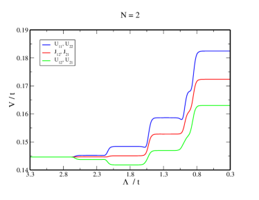
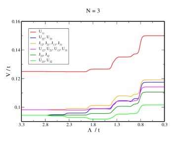
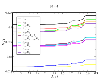
Figure 2: (color online) Flow of the coupling-functions in the zero-energy-sector of trigonal nanodiscs with $N=$2,3,4 down to a small scale around the zero-energy-states. For the parameters of the Hamiltonian (1) we set $U=3t$ and $V_{1}=2t$. The kinks of the flowing coupling-functions result from integrating out the discrete energy-levels of $\hat{H}_{0}$. In the end of the flow the coupling-functions can be interpretated as matrix elements of an effective Hamiltonian for the zero-energy-states.

Besides the single-particle energies, the parameters of the effective interaction between the zero energy states have to be determined. Here, the main parts of the Hamiltonian $\hat{H}_{\textrm{eff}}$ can be ascribed to a direct and to an exchange part. These are given by

$$\hat{H}_{\textrm{eff}}^{\textrm{dir}}= \frac{1}{2}\sum_{i_{1},i_{2}}U_{i_{1},i_{2}}\hat{n}_{i_{1}}\hat{n}_{i_{2}}$$ (49)

$$\hat{H}_{\textrm{eff}}^{\textrm{ex}}= -\sum_{\overset{i_{1},i_{2}}{i_{1}\neq i_{2}}}J_{i_{1},i_{2}}\left(\hat{\vec{S}}_{i_{1}}\hat{\vec{S}}_{i_{2}}+\frac{1}{4}\hat{n}_{i_{1}}\hat{n}_{i_{2}}\right)$$ (50)

with the matrix elements $U_{i_{1},i_{2}}=V^{\Lambda}_{i_{1},i_{2},i_{2},i_{1}}$ and $J_{i_{1},i_{2}}=V^{\Lambda}_{i_{1},i_{2},i_{1},i_{2}}$ and the spin-operators $\hat{\vec{S}}_{i}=\frac{1}{2}a^{{\dagger}}_{i,s}\vec{\sigma}_{s,s^{\prime}}a_{i,s^{\prime}}$. In Fig. 2 we show the flow of $U_{i_{1},i_{2}}$ and $J_{i_{1},i_{2}}$ as functions of the flow-parameter $\Lambda$. As can be seen these matrix elements do not change drastically during the fRG-flow, particularly for the $N=4$ system. The initial values correspond to the parameters used in the analysis of Ezawa Ezawa (2007, 2008, 2009). For $N=2$, there is a simple hierarchy. The largest couplings are the intraorbital repulsions between electrons forming a singlet in the same state. The next largest term is the spin exchange coupling, i.e. the Hund’s rule coupling, and then the interorbital repulsion. This hierarchy lets us already expect that for half filling of the zero energy levels, singly occupied orbitals are preferred and that the spins in this orbitals form the maximal total spin. For $N=3$ the picture remains similar, although now the three zero energy states consist of two states connected by the discrete rotational symmetry and another state that is strongly localized at the edges. Hence the couplings of this state (labeled ’1’) in Fig. 2. are larger than the ones that do not involve this narrow state. For a given pair of zero-energy states the hierarchy intraorbital repulsion $>$ Hund’s rule coupling $>$ interorbital repulsion is still visible. For $N=4$ the picture is more complicated. Besides these intraorbital, Hund’s rule and interorbital couplings there are other terms in $\hat{H}_{\textrm{eff}}$ that show a rather mild flow as well. By this analysis of the small nanodiscs we see that the Hartree-Fock analysis in Ezawa (2008) is already a good description of the zero-energy-sector. The problematic situation where a renormalization or splitting of the low-energy levels competes with the Hund’s rule interactions between these states does not occur. The basic aspects are captured well by ignoring the effects of the excited single-particle levels.

We can go one step further and solve the effective Hamiltonian exactly . Written as a matrix in Fock space, the effective Hamiltonian $\hat{H}_{\textrm{eff}}$ with all renormalized couplings included can be readily diagonalized. As a result we find that in trigonal zigzag-GNDs with sizes $N=2$, $3$ and $4$ the ground-state spin at half filling is equal to $S=\frac{N}{2}=\frac{L_{B}-L_{A}}{2}$. This is perfectly consistent with Lieb’s theorem. Note however that our data were obtained for nonzero nearest-neighbor interactions which is already outside the strict validity range of Lieb’s theorem.

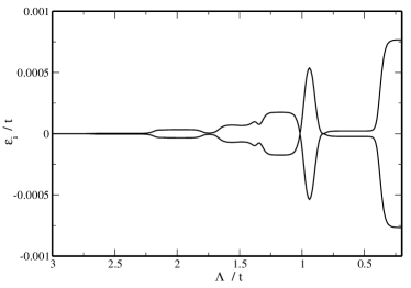
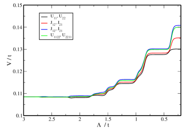
Figure 3: (color online) Flow of the one-particle-energies (upper plot) and various coupling functions (lower plot) for the bow-tie-shaped nanostructure with $\eta=2$ for $U=3t$, $V_{1}=2t$.

The situation is different in the bow-tie-shaped structures. Here the zero-energy-states split up in the fRG flow. This can be seen in the upper plot of Fig. 3. The splitting is rather small of the order of $10^{-3}t$ for our parameters. The groundstate of the free part of the effective Hamiltonian is now found to be a spin-singlet, where the single-particle state that has been renormalized down to negative energy is doubly occupied. In principle, this degeneracy-lifting of the single-particle levels due to the excited levels could compete with the effective interactions between the formerly degenerate states, in particular if there was a stronger Hund’s rule coupling between the two single-particle levels as in the $N=2$ trigonal nanodisc studied before.

Hence it is instructive and important to compare the effective Hamiltonians of the bow-tie-shaped structure and the trigonal $N=2$ nanodisc. We will see that the bow-tie ground state is indeed a singlet, but because of additional interaction terms and not because of the level splitting in the effective free part discussed just above. In both cases there are two single-particle orbitals $|1\rangle$ and $|2\rangle$. In the trigonal GND they can be distinguished by $k=\pm 2\pi/3$ while in the bow-tie-shape their $k$-indices are $k=0,\pi$ corresponding to even and odd combinations of the wavefunctions localized on primarily one side of the bow-tie whose energies are slightly split up when integrating the fRG-flow, whereat the $k=0$ state goes down in energy compared to the $k=\pi$ state.

The two-particle spin-triplet-states have the form $|\psi_{t}\rangle=\frac{1}{\sqrt{2}}\left(|1\rangle|2\rangle-|2\rangle|1\rangle\right)\chi_{t}$. In trigonal $N=2$ nanodiscs $|\psi_{t}\rangle$ forms the ground-state and the first excited states are the two degenerated singlet-states $|\psi^{1}_{sg}\rangle=|1\rangle|1\rangle\chi_{sg}$ and $|\psi^{2}_{sg}\rangle=|2\rangle|2\rangle\chi_{sg}$. The responsible term in the effective Hamiltonian is the ferromagnetic Hund’s rule-$J_{12}$ between the zero-energy states. This $J$-coupling is also positive for the bow-tie structure, as can be seen in the lower plot of Fig. 3. However, the strongest couplings that develop during the fRG-flow are however pair-hopping terms denoted by $U_{1122}$ or $U_{2211}$ of the form $\sum_{i,j}U_{iijj}a^{{\dagger}}_{i,\sigma}a^{{\dagger}}_{i,\sigma^{\prime}}a_{j,\sigma^{\prime}}a_{j,\sigma}$ in the effective Hamiltonian, and the interorbital repulsions $U_{12}=U_{21}$. Due to the latter, the spin singlet states with two electrons in the same orbital now become compatible in energy with the singly occupied states in the bow-tie-shaped structures. But the interorbital repulsion alone is not sufficient to overcome the energy gain from the Hund’s rule $J_{12}$. It is the pair-hopping term that now splits the symmetric and antisymmetric combinations of the spin singlet states $|\psi^{s}_{sg}\rangle=\frac{1}{\sqrt{2}}\left(|\psi^{1}_{sg}\rangle+|\psi^{2}_{sg}\rangle\right)$ and $|\psi^{as}_{sg}\rangle=\frac{1}{\sqrt{2}}\left(|\psi^{1}_{sg}\rangle-|\psi^{2}_{sg}\rangle\right)$, and pushes the symmetric combination $|\psi^{s}_{sg}\rangle$ below the Hund’s rule triplet $|\psi_{t}\rangle$, making the singlet the energetically most favorable spin configuration. So, instead of being exchange-driven, the singlet formation is a consequence of a pair-hopping term in the effective Hamiltonian. Note that such a pair hopping term does not occur in the effective Hamiltonian of the trigonal nanodiscs because there it is not compatible with the conservation of the $k$-quantum number characterizing the rotational symmetry of the zero-energy-states. Furthermore, if we had done the exact diagonalization without taking into account the effects of the excited single-particle levels via the fRG, the combined effects of interorbital repulsion plus pair-hopping favoring the singlet and the intraorbital repulsion plus Hund’s rule coupling would just equalize each other. This can be seen from the initial conditions for the fRG-flow of these couplings in Fig. 3, they all have the same values. This would have led us to a ground state with fluctuating total spin. Hence the bow-tie structure is a useful example that including quantum corrections by higher levels into the low-energy Hamiltonian can make a difference.

V Robustness of the zero-energy states

In the previous chapter we have seen numerically that in trigonal nanodiscs the zero-energy-states remain unsplit during the fRG-flow, while the zero-energy-states in bow-tie-shaped structures split. This can be understood more generally by an analysis of the structure of the flow equations for the selfenergy and the two-particle-vertex,

$$\Sigma^{\Lambda}\left(i_{1}^{\prime};i_{1}\right)= -\frac{1}{\beta}\sum_{i_{2},i_{2}^{\prime}}\sum_{i\omega_{n}}S^{\Lambda}_{i_{2},i_{2}^{\prime}}\left(i\omega_{n}\right)\gamma_{2}^{\Lambda}\left(i_{1}^{\prime},i_{2}^{\prime};i_{1},i_{2}\right)$$ (51)

$$\dot{\gamma}^{\Lambda}_{2}\left(i_{1}^{\prime},i_{2}^{\prime};i_{1},i_{2}\right)= \frac{1}{\beta}\sum_{i_{3},i_{3}^{\prime},i_{4},i_{4}^{\prime}}\bigg{[}\frac{1}{2}\mathcal{L}_{pp}^{\Lambda}\left(i_{3},i_{3}^{\prime};i_{4},i_{4}^{\prime}\right)$$

$$\gamma_{2}^{\Lambda}\left(i_{3}^{\prime},i_{4}^{\prime};i_{1},i_{2}\right)\gamma_{2}^{\Lambda}\left(i_{1}^{\prime},i_{2}^{\prime};i_{3},i_{4}\right)$$

$$-\mathcal{L}_{ph}^{\Lambda}(i_{3},i_{3}^{\prime};i_{4},i_{4}^{\prime})$$

$$\big{\{}\gamma_{2}^{\Lambda}\left(i_{1}^{\prime},i_{4}^{\prime};i_{1},i_{3}\right)\gamma_{2}^{\Lambda}\left(i_{3}^{\prime},i_{2}^{\prime};i_{4},i_{2}\right)$$

$$+\gamma_{2}^{\Lambda}\left(i_{2}^{\prime},i_{4}^{\prime};i_{1},i_{3}\right)\gamma_{2}^{\Lambda}\left(i_{3}^{\prime},i_{1}^{\prime};i_{4},i_{2}\right)\big{\}}\bigg{]}.$$ (52)

The loops on the right hand side are given in the appendix, Eq. (161). Furthermore, the analysis relies on a set of properties of the electronic spectrum of the free part of the Hamiltonian $\hat{H}_{0}=-t\sum_{\langle i,j\rangle,\sigma}\left(c^{{\dagger}}_{i,\sigma}c_{j,\sigma}+h.c.\right)$.

Let $|A\rangle$ and $|B\rangle$ denote states that have only nonzero weight on $A$ and $B$ sublattice, respectively. Then a realspace-operator $\mathcal{O}$ shall be denoted as odd if it has only nonzero matrix elements of the form $\langle A|\mathcal{O}|B\rangle$ or $\langle B|\mathcal{O}|A\rangle$. Similarly, an operator $\mathcal{E}$ that has only nonzero matrix elements of the form $\langle A|\mathcal{E}|A\rangle$ or $\langle B|\mathcal{E}|B\rangle$ is denoted as even. Note, that an odd operator with real matrix elements is particle-hole-symmetric, i.e. invariant under the transformation $a_{i}\rightarrow\xi_{i}a^{{\dagger}}_{i}$ with $\xi_{i}=1$ if the site i belongs to sublattice A and $\xi_{i}=-1$ if the site i belongs to sublattice B. The free Hamiltonian $\hat{H_{0}}$ is odd. Therefore the rank of the matrix $\hat{H_{0}}$ is at most $2L_{A}$ and the nullity of $\hat{H_{0}}$, which is equal to the number of zero-energy-states, is $\eta=L_{A}+L_{B}-\text{rank}\left(\hat{H_{0}}\right)\geq L_{B}-L_{A}$ Lieb (1989), which is consistent with the statements about the number of zero-energy-states given before. Note, that there are at least $L_{B}-L_{A}$ zero-energy-states resulting from the sublattice-imbalance. Let $|E\rangle=|A\rangle+|B\rangle$ be one of the remaining $2L_{A}$ eigenvectors of $\hat{H_{0}}$ with energy $E$ (whereat the case $E=0$ is also possible). Then $|-E\rangle=|A\rangle-|B\rangle$ is also an eigenvector of $\hat{H_{0}}$ with energy $-E$. Therefore the remaining energies come in pairs $\pm E$. The symmetric and antisymmetric linear combinations $|s\rangle=\frac{1}{\sqrt{2}}(|E\rangle+|-E\rangle)$ and $|as\rangle=\frac{1}{\sqrt{2}}(|E\rangle-|-E\rangle)$ are fully sublattice-polarized, i.e. $|s\rangle\in A$ and $|as\rangle\in B$. The symmetric and antisymmetric combinations that can be formed from the $L_{B}-L_{A}$ zero-energy-states resulting from the sublattice-imbalance either vanish or are fully sublattice-polarized on sublattice $B$, because the $L_{A}$ symmetric states form a basis for the states on sublattice $A$ and the zero-energy-states are linearly independent on them.

In the following we assume that there are no initial interactions of the form $V(i\in A,j\in A;k\in A,l\in B)$ or $V(i\in B,j\in B;k\in B,l\in A)$ (and cyclic), which is the case in the Hamiltonian (1). By this we show that the selfenergy that is odd initially remains odd under the fRG-flow and the zero-energy degeneracy resulting from the sublattice-imbalance is conserved.

The transformation matrix from the eigenbasis of $\hat{H_{0}}$ into the basis of the symmetric and antisymmetric states is given by

$$V_{0}=\left[\begin{array}[]{c|c|c|c}&+&-&0\\ \hline\cr s&\frac{1}{\sqrt{2}}\mathbbm{1}&\frac{1}{\sqrt{2}}\mathbbm{1}&\\ \hline\cr as&\frac{1}{\sqrt{2}}\mathbbm{1}&-\frac{1}{\sqrt{2}}\mathbbm{1}&\\ \hline\cr 0&&&\mathbbm{1}\end{array}\right]$$ (57)

where ”+”, ”-” and ”0” denote the sector of positive, negative and zero energies. Empty fields are filled with zero matrices of appropriate size. The transformation matrix from this (s/as)-space into the real space has the form

$$W_{0}=\left[\begin{array}[]{c|c|c|c}&s&as&0\\ \hline\cr A&&\ast&\\ \hline\cr B&\ast&&\ast\end{array}\right].$$ (61)

where ”$\ast$” represent an arbitrary matrix block. The general form of odd and even matrices in the (s/as)-space is

$$\mathcal{E}_{s/as}=\left[\begin{array}[]{c|c|c|c}&s&as&0\\ \hline\cr s&\ast&&\ast\\ \hline\cr as&&\ast&\\ \hline\cr 0&\ast&&\ast\end{array}\right],\mathcal{O}_{s/as}=\left[\begin{array}[]{c|c|c|c}&s&as&0\\ \hline\cr s&&\ast&\\ \hline\cr as&\ast&&\ast\\ \hline\cr 0&&\ast&\end{array}\right]$$ (70)

In the eigenbasis of $\hat{H_{0}}$ the cutoff-matrix $\chi^{\Lambda}$ has the form

$$\chi^{\Lambda}=\left[\begin{array}[]{c|c|c|c}&+&-&0\\ \hline\cr+&\chi^{\Lambda}_{++}&&\\ \hline\cr-&&\chi^{\Lambda}_{--}&\\ \hline\cr 0&&&\ast\end{array}\right],$$ (75)

with diagonal matrices $\chi^{\Lambda}_{++}=\chi^{\Lambda}_{--}$. By transforming this matrix into the (s/as)-space $\chi^{\Lambda}_{s/as}=V_{0}\chi^{\Lambda}V_{0}^{{\dagger}}$ has the same form as $\mathcal{E}_{s/as}$ and is therefore even. Analogously it follows that $\left(\chi^{\Lambda}\right)^{1/2}$ and $\dot{\chi}^{\Lambda}\left(\chi^{\Lambda}\right)^{-1}=\tilde{\beta}\left(\mathbbm{1}-\chi^{\Lambda}\right)$ are even.

In the following we will first show that the frequency-integrated single-scale propagator (see (44) and (A)) is odd if we assume that the selfenergy is odd. From the structure of the flow equation (51) it can be seen that the selfenergy remains odd during the fRG-flow if no two-particle-vertices of the form $\gamma^{\Lambda}_{2}\left(i\in A,j\in A;k\in A,l\in B\right)$ or $\gamma^{\Lambda}_{2}\left(i\in B,j\in B;k\in B,l\in A\right)$ (and cyclic) are generated in the flow equations (51). In a second step we show that these vertices will not occur, if there are no initial interactions of this form (as is assumed further above).

Step 1: Analysis of the frequency integrated single-scale propagator

If we assume that the selfenergy $\Sigma^{\Lambda}$ is odd, the matrix $\hat{H}_{0}+\left(\chi^{\Lambda}\right)^{1/2}\Sigma^{\Lambda}\left(\chi^{\Lambda}\right)^{1/2}$ is odd and has a symmetric spectrum. Analogue to the case of $\hat{H}_{0}$ we can transform its eigenstates into symmetrized and antisymmetrized states. The transformation-matrices $W$ and $V$ have the same structure as $W_{0}$ and $V_{0}$.

The first term of the frequency-integrated single-scale propagator (A) is

$$\left(\chi^{\Lambda}\right)^{1/2}\dot{\chi}^{\Lambda}\left(\chi^{\Lambda}\right)^{-1}UFU^{\dagger}\left(\chi^{\Lambda}\right)^{1/2}$$

$$= \left(\chi^{\Lambda}\right)^{1/2}\dot{\chi}^{\Lambda}\left(\chi^{\Lambda}\right)^{-1}WF_{s/as}W^{\dagger}\left(\chi^{\Lambda}\right)^{1/2},$$ (76)

with the matrix $F$ given by

$$F_{a,b}=\left(n_{F}(E_{a})-\frac{1}{2}\right)\delta_{a,b}$$ (77)

In the eigenspace of $\hat{H}_{0}+\left(\chi^{\Lambda}\right)^{1/2}\Sigma^{\Lambda}\left(\chi^{\Lambda}\right)^{1/2}$ the matrix $F$ has the form

$$F=\left[\begin{array}[]{c|c|c|c}&+&-&0\\ \hline\cr+&F_{++}&&\\ \hline\cr-&&F_{--}&\\ \hline\cr 0&&&\end{array}\right],$$ (82)

with $F_{++}=-F_{--}$. In the (s/as)-space $F_{s/as}=VFV^{{\dagger}}$ has the same structure as $\mathcal{O}_{s/as}$ and is therefore odd. Since the remaining matrices in (V) are even, the first term of the frequency-integrated single-scale propagator is odd.

The second term of the frequency-integrated single-scale propagator is

$$\left(\chi^{\Lambda}\right)^{1/2}UCU^{\dagger}\left(\chi^{\Lambda}\right)^{1/2}$$

$$= \left(\chi^{\Lambda}\right)^{1/2}WC_{s/as}W^{\dagger}\left(\chi^{\Lambda}\right)^{1/2},$$

with the matrix C given by

$$C_{a,b}=\mathcal{F}^{+}_{a,b}\left[U^{\dagger}\tilde{D}U\right]_{a,b}$$ (83)

where $\tilde{D}=\left(\chi^{\Lambda}\right)^{1/2}\Sigma^{\Lambda}\left(\chi^{\Lambda}\right)^{1/2}\dot{\chi}^{\Lambda}\left(\chi^{\Lambda}\right)^{-1}$

In the eigenspace of $\hat{H}_{0}+\left(\chi^{\Lambda}\right)^{1/2}\Sigma^{\Lambda}\left(\chi^{\Lambda}\right)^{1/2}$ the matrix $\mathcal{F}^{+}$ has the structure

$$\mathcal{F}^{+}=\left[\begin{array}[]{c|c|c|c}&+&-&0\\ \hline\cr+&\mathcal{F}^{+}_{++}&\mathcal{F}^{+}_{+-}&\mathcal{F}^{+}_{+0}\\ \hline\cr-&\mathcal{F}^{+}_{-+}&\mathcal{F}^{+}_{--}&\mathcal{F}^{+}_{-0}\\ \hline\cr 0&\mathcal{F}^{+}_{0+}&\mathcal{F}^{+}_{0-}&\ast\end{array}\right],$$ (88)

with $\mathcal{F}^{+}_{++}=\mathcal{F}^{+}_{--}$, $\mathcal{F}^{+}_{+-}=\mathcal{F}^{+}_{-+}$, $\mathcal{F}^{+}_{0+}=\mathcal{F}^{+}_{0-}$ and $\mathcal{F}^{+}_{+0}=\mathcal{F}^{+}_{-0}$.

The matrix $\tilde{D}=\left(\chi^{\Lambda}\right)^{1/2}\Sigma^{\Lambda}\left(\chi^{\Lambda}\right)^{1/2}\dot{\chi}^{\Lambda}\left(\chi^{\Lambda}\right)^{-1}$ is odd and therefore the matrix $D=U^{\dagger}\tilde{D}U$ has the structure

$$D=\left[\begin{array}[]{c|c|c|c}&+&-&0\\ \hline\cr+&D_{++}&D_{+-}&D_{+0}\\ \hline\cr-&D_{-+}&D_{--}&D_{-0}\\ \hline\cr 0&D_{0+}&D_{0-}&\end{array}\right]$$ (93)

where $D_{++}=-D_{--}$, $D_{+-}=-D_{-+}$, $D_{0+}=-D_{0-}$ and $D_{+0}=-D_{-0}$. So $D$ has the same form as $V\mathcal{O}_{s/as}V^{{\dagger}}$ and is therefore odd.

The structure of the matrix $C$ in the eigenspace of $\hat{H}_{0}+\left(\chi^{\Lambda}\right)^{1/2}\Sigma^{\Lambda}\left(\chi^{\Lambda}\right)^{1/2}$ is then

$$C=\left[\begin{array}[]{c|c|c|c}&+&-&0\\ \hline\cr+&C_{++}&C_{+-}&C_{+0}\\ \hline\cr-&C_{-+}&C_{--}&C_{-0}\\ \hline\cr 0&C_{0+}&C_{0-}&\end{array}\right],$$ (98)

with $C_{++}=-C_{--}$, $C_{+-}=-C_{-+}$, $C_{0+}=-C_{0-}$ and $C_{+0}=-C_{-0}$. The matrix $C_{s/as}=VCV^{{\dagger}}$ has the same structure as $\mathcal{O}_{s/as}$ and is therefore odd. By this we see that the second summand of the frequency-integrated single-scale propagator is also odd.

In summary it follows that the single-scale propagator (A) is odd, when we assume that the selfenergy is odd.

Step 2: Analysis of the flow equation for the two-particle-vertex

In the second step of our proof, we will now show that no two-particle-vertices of the form $\gamma^{\Lambda}_{2}\left(i\in A,j\in A;k\in A,l\in B\right)$ or $\gamma^{\Lambda}_{2}\left(i\in B,j\in B;k\in B,l\in A\right)$ (and cyclic) are generated in the flow equations (52). We assume that there are no initial interactions of the form $V(i\in A,j\in A;k\in A,l\in B)$ or $V(i\in B,j\in B;k\in B,l\in A)$ (and cyclic). From the structure of the flow equations (52) it can be seen, that no vertices of the indicated form are generated, if there are no Matsubara-sums (161) of the form $\mathcal{L}^{\Lambda}_{pp/ph}\left(q\in A,q^{\prime}\in A;k\in A,k^{\prime}\in B\right)$ or $\mathcal{L}^{\Lambda}_{pp/ph}\left(q\in B,q^{\prime}\in B;k\in B,k^{\prime}\in A\right)$ (and cyclic).

The Matsubara-sum of the particle-hole-channel can be written in the form

$$\mathcal{L}^{\Lambda}_{ph}(q,q^{\prime};k,k^{\prime})= -\sum_{i\omega_{n}}\bigg{\{}\dot{\mathcal{G}}^{\Lambda}_{k,k^{\prime}}(i\omega_{n})\mathcal{G}^{\Lambda}_{q,q^{\prime}}(i\omega_{n})$$

$$+\dot{\mathcal{G}}^{\Lambda}_{q,q^{\prime}}(i\omega_{n})\mathcal{G}^{\Lambda}_{k,k^{\prime}}(i\omega_{n})\bigg{\}}$$

$$= -\frac{\textrm{d}}{\textrm{d}\Lambda}\sum_{i\omega_{n}}\mathcal{G}^{\Lambda}_{k,k^{\prime}}(i\omega_{n})\mathcal{G}^{\Lambda}_{q,q^{\prime}}(i\omega_{n}).$$ (99)

By achieving the Matsubara-sum we get

$$\mathcal{L}^{\Lambda}_{ph}(q,q^{\prime};k,k^{\prime})= \beta\frac{\textrm{d}}{\textrm{d}\Lambda}\sum_{a,b}\left[\left(\chi^{\Lambda}\right)^{1/2}U\right]_{k,a}\left[\left(\chi^{\Lambda}\right)^{1/2}U\right]_{q,b}$$

$$\mathcal{F}^{+}_{a,b}\left[U^{\dagger}\left(\chi^{\Lambda}\right)^{1/2}\right]_{a,k^{\prime}}\left[U^{\dagger}\left(\chi^{\Lambda}\right)^{1/2}\right]_{b,q^{\prime}}$$

$$= \beta\frac{\textrm{d}}{\textrm{d}\Lambda}\sum_{a,a^{\prime},b,b^{\prime}}\left[\left(\chi^{\Lambda}\right)^{1/2}U\right]_{k,a}\left[\left(\chi^{\Lambda}\right)^{1/2}U\right]_{q,b}$$

$$\overbrace{\mathcal{F}^{+}_{a,b}\delta_{a,a^{\prime}}\delta_{b,b^{\prime}}}^{\tilde{\mathcal{F}}_{a,b,a^{\prime},b^{\prime}}^{+}}$$

$$\left[U^{\dagger}\left(\chi^{\Lambda}\right)^{1/2}\right]_{a^{\prime},k^{\prime}}\left[U^{\dagger}\left(\chi^{\Lambda}\right)^{1/2}\right]_{b^{\prime},q^{\prime}}$$

$$= \beta\frac{\textrm{d}}{\textrm{d}\Lambda}\sum_{\alpha,\alpha^{\prime},\beta,\beta^{\prime}}\left[\left(\chi^{\Lambda}\right)^{1/2}W\right]_{k,\alpha}$$

$$\left[\left(\chi^{\Lambda}\right)^{1/2}W\right]_{q,\beta}\left[\tilde{\mathcal{F}}^{+}_{s/as}\right]_{\alpha,\beta,\alpha^{\prime},\beta^{\prime}}$$

$$\left[W^{\dagger}\left(\chi^{\Lambda}\right)^{1/2}\right]_{\alpha^{\prime},k^{\prime}}\left[W^{\dagger}\left(\chi^{\Lambda}\right)^{1/2}\right]_{\beta^{\prime},q^{\prime}}.$$ (100)

In the (s/as)-space $\tilde{\mathcal{F}}^{+}_{s/as}$ has the form

$$\begin{array}[]{lll}\left[\tilde{\mathcal{F}}^{+}_{s/as}\right]_{.,.,s,s}=&\left[\tilde{\mathcal{F}}^{+}_{s/as}\right]_{.,.,s,as}=&\left[\tilde{\mathcal{F}}^{+}_{s/as}\right]_{.,.,s,0}=\\ \left[\begin{array}[]{c|c|c|c}&s&as&0\\ \hline\cr s&\ast&&\\ \hline\cr as&&\ast&\\ \hline\cr 0&&&\end{array}\right]&\left[\begin{array}[]{c|c|c|c}&s&as&0\\ \hline\cr s&&\ast&\\ \hline\cr as&\ast&&\\ \hline\cr 0&&&\end{array}\right]&\left[\begin{array}[]{c|c|c|c}&s&as&0\\ \hline\cr s&&&\ast\\ \hline\cr as&&&\\ \hline\cr 0&&&\end{array}\right]\\ &&\\ \left[\tilde{\mathcal{F}}^{+}_{s/as}\right]_{.,.,as,s}=&\left[\tilde{\mathcal{F}}^{+}_{s/as}\right]_{.,.,as,as}=&\left[\tilde{\mathcal{F}}^{+}_{s/as}\right]_{.,.,as,0}=\\ \left[\begin{array}[]{c|c|c|c}&s&as&0\\ \hline\cr s&&\ast&\\ \hline\cr as&\ast&&\\ \hline\cr 0&&&\end{array}\right]&\left[\begin{array}[]{c|c|c|c}&s&as&0\\ \hline\cr s&\ast&&\\ \hline\cr as&&\ast&\\ \hline\cr 0&&&\end{array}\right]&\left[\begin{array}[]{c|c|c|c}&s&as&0\\ \hline\cr s&&&\\ \hline\cr as&&&\ast\\ \hline\cr 0&&&\end{array}\right]\\ &&\\ \left[\tilde{\mathcal{F}}^{+}_{s/as}\right]_{.,.,0,s}=&\left[\tilde{\mathcal{F}}^{+}_{s/as}\right]_{.,.,0,as}=&\left[\tilde{\mathcal{F}}^{+}_{s/as}\right]_{.,.,0,0}=\\ \left[\begin{array}[]{c|c|c|c}&s&as&0\\ \hline\cr s&&&\\ \hline\cr as&&&\\ \hline\cr 0&\ast&&\end{array}\right]&\left[\begin{array}[]{c|c|c|c}&s&as&0\\ \hline\cr s&&&\\ \hline\cr as&&&\\ \hline\cr 0&&\ast&\end{array}\right]&\left[\begin{array}[]{c|c|c|c}&s&as&0\\ \hline\cr s&&&\\ \hline\cr as&&&\\ \hline\cr 0&&&\ast\end{array}\right],\end{array}$$ (145)

which can be easily seen by a transformation with V. In the realspace the matrix has the form

$$\begin{array}[]{ll}\left[\tilde{\mathcal{F}}_{pos}^{+}\right]_{.,.,A,A}=\left[\begin{array}[]{c|c|c}&A&B\\ \hline\cr A&\ast&\\ \hline\cr B&&\ast\end{array}\right]&\left[\tilde{\mathcal{F}}_{pos}^{+}\right]_{.,.,A,B}=\left[\begin{array}[]{c|c|c}&A&B\\ \hline\cr A&&\ast\\ \hline\cr B&\ast&\end{array}\right]\\ \left[\tilde{\mathcal{F}}_{pos}^{+}\right]_{.,.,B,A}=\left[\begin{array}[]{c|c|c}&A&B\\ \hline\cr A&&\ast\\ \hline\cr B&\ast&\end{array}\right]&\left[\tilde{\mathcal{F}}_{pos}^{+}\right]_{.,.,B,B}=\left[\begin{array}[]{c|c|c}&A&B\\ \hline\cr A&\ast&\\ \hline\cr B&&\ast\end{array}\right].\end{array}$$ (160)

We see that there are no expressions of the indicated form and hence no vertexfunctions of the form $\gamma^{\Lambda}_{2}\left(i\in A,j\in A;k\in A,l\in B\right)$ or $\gamma^{\Lambda}_{2}\left(i\in B,j\in B;k\in B,l\in A\right)$ (and cyclic) are generated in the flow equations (52). The analysis of the particle-particle-channel is analogous.

In summary we have seen that when we neglect the frequency dependence of the vertexfunctions and truncate the fRG-equations (as usual) by setting $\gamma_{\geq 3}^{\Lambda}\equiv 0$, the selfenergy remains odd during the fRG-flow and the high zero-energy-degeneracy, following from the sublattice imbalance is conserved. This result is not restricted to a special geometry or size of the GNDs. For the bow-tie-shaped structure, the sublattice imbalance is zero and therefore there are no protected single-particle levels with zero energy. Note, that within this approximation the calculated selfenergy is particle-hole-symmetric, although the initial interactions do not have to be particle-hole-symmetric. A nearest-neighbor interaction like in (1) is for example not particle-hole-symmetric, but anyway the corresponding initial conditions contain no coupling-functions of the form $V(i\in A,j\in A;k\in A,l\in B)$ or $V(i\in B,j\in B;k\in B,l\in A)$ (and cyclic).

VI Conclusions

We have described a general fRG framework to to derive effective Hamiltonians for the low-lying states of finite-size or nanostructured lattice systems. It allows one to assess the influence of empty or filled single-particle states away from the Fermi level on the spectrum and the interactions of the degrees of freedom near the Fermi level. With the resulting effective Hamiltonian at hand, we have then performed exact diagonalization studies of the effective Hamiltonians in order to determine the ground-state spin of trigonal nanodiscs and bow-tie-shaped structures. Of course, other properties like transport can also be studied using the effective description delivered by the fRG.

The application of the fRG scheme to different smaller nanodiscs showed that there are two classes of nanodiscs (assuming nearest-neighbor hopping only). One class has nonzero sublattice imbalance equal to the number of zero-energy states $\eta$. Here the zero-energy single-particle levels are protected under integrating out the excited single-particle levels. The results in the literatureEzawa (2007, 2008, 2009) that were obtained by neglecting the renormalizations by the higher levels are hence found to be valid. The protection of the zero-energy levels can be understood analytically for arbitrary $N$ and also holds for other geometries with sub-lattice imbalance. If the zero-energy states occur for zero sublattice-imbalance, as for the bow-tie nanodisc, they can split up under the fRG flow, and at least in principle the splitting may influence the low-energy picture, in particular if it gets large compared to the effective interactions between these states. In the cases studied here, the splitting on the single-particle level remained small and was clearly dominated by interaction effects.

In our applications of the method to trigonal nanodiscs the inclusion of the excited states turned out to be at most a quantitative effect. Here, the large-spin ground state discussed in the literature is not altered by the renormalization. Also, the small degeneracy lifting of the single-particle levels in the bow-tie structures $\sim 10^{-3}t\sim 2meV$ is in principle observable but it will be dominated by interaction effects. The renormalization of the effective interactions is also quite moderate. Nevertheless, our analysis of the bow-tie structures shows that integrating out the excited levels in the fRG flow tips the balance in the effective interactions toward a spin singlet rather than selecting the Hund’s rule triplet. The fRG flow of the pair-hopping term between the effective orbitals turns out to be stronger than that of the spin-exchange interaction. This nicely demonstrates the usefulness of the renormalization group in situations of competing trends.

The numerical implementation of the functional renormalization group scheme to these small systems is straightforward and one could imagine many other fields of applications. Another possible example with interesting low-energy states are conducting edge states of wires with gapped bulk spectrum, where the bulk states could be integrated out yielding the nontrivial effective description of the edge states only. However, for larger systems than the ones studied here, the effective interactions should be truncated in range or parameterized differently, otherwise the numerical effort becomes significant.

We thank Sabine Andergassen, Fakher Assaad, Motohiko Ezawa, Volker Meden, Manfred Salmhofer, Jacob Schmiedt for useful discussions, and Björn Trauzettel for drawing our attention to graphene nanodiscs.

Appendix A Evalulation of Matsubara-sums

The truncated flowequations for the vertexfunctions $\Sigma^{\Lambda}$ and $\gamma_{2}^{\Lambda}$ are given in the main text, eqs. (52). Here

$$\mathcal{L}_{pp}^{\Lambda}\left(i_{3},i_{3}^{\prime};i_{4},i_{4}^{\prime}\right)= \sum_{i\omega_{n}}\bigg{[}S^{\Lambda}_{i_{4},i_{4}^{\prime}}\left(i\omega_{n}\right)\mathcal{G}^{\Lambda}_{i_{3},i_{3}^{\prime}}\left(-i\omega_{n}\right)$$

$$+S^{\Lambda}_{i_{3},i_{3}^{\prime}}\left(i\omega_{n}\right)\mathcal{G}^{\Lambda}_{i_{4},i_{4}^{\prime}}\left(-i\omega_{n}\right)\bigg{]}$$

$$\mathcal{L}_{ph}^{\Lambda}\left(i_{3},i_{3}^{\prime};i_{4},i_{4}^{\prime}\right)= \sum_{i\omega_{n}}\bigg{[}S^{\Lambda}_{i_{4},i_{4}^{\prime}}\left(i\omega_{n}\right)\mathcal{G}^{\Lambda}_{i_{3},i_{3}^{\prime}}\left(i\omega_{n}\right)$$

$$+S^{\Lambda}_{i_{3},i_{3}^{\prime}}\left(i\omega_{n}\right)\mathcal{G}^{\Lambda}_{i_{4},i_{4}^{\prime}}\left(i\omega_{n}\right)\bigg{]}$$ (161)

The Matsubara-sums in (51) and (161) can be calculated analytically. Therefore we write the Single-Scale-Propagator as

$$S^{\Lambda}\left(i\omega_{n}\right)= -\bigg{\{}\left(\chi^{\Lambda}\right)^{1/2}\dot{\chi}^{\Lambda}\left(\chi^{\Lambda}\right)^{-1}$$

$$\times\left[\mathcal{G}_{0}^{-1}\left(i\omega_{n}\right)-\left(\chi^{\Lambda}\right)^{1/2}\Sigma^{\Lambda}\left(\chi^{\Lambda}\right)^{1/2}\right]^{-1}$$

$$+\left(\chi^{\Lambda}\right)^{1/2}\left[\mathcal{G}_{0}^{-1}\left(i\omega_{n}\right)-\left(\chi^{\Lambda}\right)^{1/2}\Sigma^{\Lambda}\left(\chi^{\Lambda}\right)^{1/2}\right]^{-1}$$

$$\times\left(\chi^{\Lambda}\right)^{1/2}\Sigma^{\Lambda}\left(\chi^{\Lambda}\right)^{1/2}\dot{\chi}^{\Lambda}\left(\chi^{\Lambda}\right)^{-1}$$

$$\times\left[\mathcal{G}_{0}^{-1}\left(i\omega_{n}\right)-\left(\chi^{\Lambda}\right)^{1/2}\Sigma^{\Lambda}\left(\chi^{\Lambda}\right)^{1/2}\right]^{-1}\left(\chi^{\Lambda}\right)^{1/2}\bigg{\}}$$ (162)

Let U be the ($\Lambda$-dependent) transformationmatrix from the eigenspace of $\hat{H}_{0}+\left(\chi^{\Lambda}\right)^{1/2}\Sigma^{\Lambda}\left(\chi^{\Lambda}\right)^{1/2}$ in the realspace. The Matsubara-sum in (51) can then be translated into a contour-integral in the complex plane and solved by the residue-theorem. The result is

$$\sum_{i\omega_{n}}S^{\Lambda}_{i_{2},i_{2}^{\prime}}\left(i\omega_{n}\right)= \beta\bigg{\{}\sum_{a}\left[\left(\chi^{\Lambda}\right)^{1/2}\dot{\chi}^{\Lambda}\left(\chi^{\Lambda}\right)^{-1}U\right]_{i_{2},a}$$

$$\times\left(n_{F}(E_{a})-\frac{1}{2}\right)\left[U^{\dagger}\left(\chi^{\Lambda}\right)^{1/2}\right]_{a,i_{2}^{\prime}}$$

$$+\sum_{a,b}\left[\left(\chi^{\Lambda}\right)^{1/2}U\right]_{i_{2},a}\mathcal{F}_{a,b}^{+}$$

$$\times\left[U^{\dagger}\left(\chi^{\Lambda}\right)^{1/2}\Sigma^{\Lambda}\left(\chi^{\Lambda}\right)^{1/2}\dot{\chi}^{\Lambda}\left(\chi^{\Lambda}\right)^{-1}U\right]_{a,b}$$

$$\times\left[U^{\dagger}\left(\chi^{\Lambda}\right)^{1/2}\right]_{b,i_{2}^{\prime}}\bigg{\}}$$ (163)

with

$$\mathcal{F}_{a,b}^{\pm}=\begin{cases}n_{F}^{\prime}(E_{a})&\text{if}\quad E_{a}=\pm E_{b}\\ \frac{n_{F}(E_{a})-n_{F}(\pm E_{b})}{E_{a}\mp E_{b}}&\text{if}\quad E_{a}\neq\pm E_{b}\end{cases}$$ (164)

In the contour-integral we used the function $n_{F}(\omega)-1/2$ instead of a normal fermifunction. In the Matsubara-sums (161) we replace the free propagator $\mathcal{G}_{0}^{\Lambda}$ by the full-propagator (Katanin-like refinement)Katanin (2004). After the contourintegration we get

$$\mathcal{L}^{\Lambda}_{\overset{pp}{ph}}= \beta\sum_{a,b}\bigg{\{}\left[\dot{\left(\chi^{\Lambda}\right)}^{1/2}U\right]_{q,a}\left[U^{\dagger}\left(\chi^{\Lambda}\right)^{1/2}\right]_{a,q^{\prime}}$$

$$+\left[\left(\chi^{\Lambda}\right)^{1/2}U\right]_{q,a}\left[U^{\dagger}\dot{\left(\chi^{\Lambda}\right)}^{1/2}\right]_{a,q^{\prime}}\bigg{\}}$$

$$\times\mathcal{F}_{a,b}^{\mp}\left[\left(\chi^{\Lambda}\right)^{1/2}U\right]_{s,b}\left[U^{\dagger}\left(\chi^{\Lambda}\right)^{1/2}\right]_{b,s^{\prime}}$$

$$+\beta\sum_{a,b,c}\left[\left(\chi^{\Lambda}\right)^{1/2}U\right]_{q,a}\left[U^{\dagger}K^{\Lambda}U\right]_{a,b}$$

$$\left[U^{\dagger}\left(\chi^{\Lambda}\right)^{1/2}\right]_{b,q^{\prime}}\left[\left(\chi^{\Lambda}\right)^{1/2}U\right]_{s,c}\left[U^{\dagger}\left(\chi^{\Lambda}\right)^{1/2}\right]_{c,s^{\prime}}\mathcal{E}_{a,b,c}^{\mp}$$

$$+\big{[}q\leftrightarrow s\big{]}\big{[}q^{\prime}\leftrightarrow s^{\prime}\big{]}$$ (165)

with

$$K^{\Lambda}= \dot{\left(\chi^{\Lambda}\right)}^{1/2}\Sigma^{\Lambda}\left(\chi^{\Lambda}\right)^{1/2}+\left(\chi^{\Lambda}\right)^{1/2}\dot{\Sigma}^{\Lambda}\left(\chi^{\Lambda}\right)^{1/2}$$

$$+\left(\chi^{\Lambda}\right)^{1/2}\Sigma^{\Lambda}\dot{\left(\chi^{\Lambda}\right)}^{1/2}$$ (166)

and the matrix

$$\mathcal{E}^{\pm}_{a,b,c}=$$

$$\begin{cases}n_{F}^{\prime\prime}(E_{a})&\text{if}\quad E_{a}=E_{b}=\mp E_{c}\\ \frac{n_{F}(\mp E_{c})-n_{F}(E_{a})}{(E_{a}\mp E_{c})^{2}}+\frac{n_{F}^{\prime}(E_{a})}{E_{a}\mp E_{c}}&\text{if}\quad E_{a}=E_{b}\neq\mp E_{c}\\ \frac{n_{F}(E_{b})-n_{F}(E_{a})}{(E_{a}-E_{b})^{2}}+\frac{n_{F}^{\prime}(E_{a})}{E_{a}-E_{b}}&\text{if}\quad E_{a}=\mp E_{c}\neq E_{b}\\ \frac{n_{F}(E_{a})-n_{F}(E_{b})}{(E_{a}-E_{b})^{2}}+\frac{n_{F}^{\prime}(E_{b})}{E_{b}-E_{a}}&\text{if}\quad E_{b}=\mp E_{c}\neq E_{a}\\ \frac{n_{F}(E_{a})}{(E_{a}-E_{b})(E_{a}\mp E_{c})}+\frac{n_{F}(E_{b})}{(E_{b}-E_{a})(E_{b}\mp E_{c})}\\ +\frac{n_{F}(\mp E_{c})}{(\mp E_{c}-E_{a})(\mp E_{c}-E_{b})}&\text{if}\quad E_{a}\neq E_{b}\neq\mp E_{c}\neq E_{a}\end{cases}$$ (167)

References

• Ezawa (2009) M. Ezawa, Eur. Phys. J. B 67, 543 (2009).
• Fernández-Rossier and Palacios (2007) J. Fernández-Rossier and J. Palacios, Phys. Rev. Lett. 99, 177204 (2007).
• Wang et al. (2009) W. L. Wang, O. B. Yazyev, S. Meng, and E. Kaxiras, Phys. Rev. Lett. 102, 157201 (2009).
• Ezawa (2007) M. Ezawa, Phys. Rev. B 76, 245415 (2007).
• Fajtlowicz et al. (2005) S. Fajtlowicz, P. E. John, and H. Sachs, Croatica Chemica Acta 78, 195 (2005).
• Wang et al. (2008) W. L. Wang, S. Meng, and E. Kaxiras, Nano Lett 8, 241 (2008).
• Lieb (1989) E. H. Lieb, Phys. Rev. Lett. 62, 1201 (1989).
• Ezawa (2008) M. Ezawa, Phys. Rev. B 77, 155411 (2008).
• Zanchi and Schulz (1998) D. Zanchi and H. Schulz, Europhys. Lett. 44, 235 (1998).
• Zanchi and Schulz (2000) D. Zanchi and H. J. Schulz, Phys. Rev. B 61, 13609 (2000).
• Halboth and Metzner (2000) C. J. Halboth and W. Metzner, Phys. Rev. B 61, 7364 (2000).
• Honerkamp et al. (2001) C. Honerkamp, M. Salmhofer, N. Furukawa, and T. M. Rice, Phys. Rev. B 63, 035109 (2001).
• Andergassen et al. (2004) S. Andergassen, T. Enss, V. Meden, W. Metzner, U. Schollwöck, and K. Schönhammer, Phys. Rev. B 70, 075102 (2004).
• Meden et al. (2008) V. Meden, S. Andergassen, T. Enss, H. Schoeller, and K. Schönhammer, New Journal of Physics 10, 045012 (23pp) (2008).
• Morris (1994) T. Morris, Int. J. Mod. Phys. 9, 2411 (1994).
• Salmhofer (1999) M. Salmhofer, Renormalization. An Introduction (Springer, 1999).
• Wetterich (1993) C. Wetterich, Phys. Lett. B 301, 90 (1993).
• Salmhofer and Honerkamp (2001) M. Salmhofer and C. Honerkamp, Progress in Theoretical Physics 105, 1 (2001).
• Katanin (2004) A. A. Katanin, Phys. Rev. B 70, 115109 (2004).