Statistical measure of complexity of hard-sphere gas: applications to nuclear matter

Abstract

We apply the statistical measure of complexity, introduced by López-Ruiz, Mancini and Calbet to a hard-sphere dilute Fermi gas whose particles interact via a repulsive hard-core potential. We employ the momentum distribution of this system to calculate the information entropy, the disequilibrium and the statistical complexity. We examine possible connections between the particle correlations and energy of the system with those information and complexity measures. The hard-sphere model serves as a test bed for concepts about complexity.

PACS number(s): 05.30.Fk, 89.70.Cf, 05.30.-d, 05.90.+m

Keywards: Momentum Distribution, Fermi Systems, Nuclear Matter, Hard-Sphere Gas, Information Entropy, Statistical Complexity, Correlations.

1 Introduction

There has been a remarkable growth in research focused on complexity and in general on information theories in recent years in a variety of fields [1] including physics [2], chemistry [3], biology [4], neuroscience [5], mathematics [6] and computer science [7]. In particular there are various applications in quantum many-body systems e.g. atoms [8, 9, 10], nuclei [11, 12, 13, 14], atomic clusters [12], bosonic traps [12] e.t.c. In fact, they lead to the clarification of basic quantum concepts and provide results about the information content of systems according to various definitions e.g. Shannon information entropy [15], Fisher [16] information, Onicescu information energy [17] e.t.c. Also they represent a suitable framework, via a probabilistic description, to assess the presence of interactions, correlations with experimentally measurable quantities, the derivation of universal relations e.t.c [11, 12, 13, 15, 16, 17, 18, 19, 20, 21, 22, 23, 24, 25, 26, 27, 28, 29, 30, 31, 32]. Thus, traditional methods can be extended by an alternative information-theoretic way and give new insights for the treatment of simple quantum systems as well as more complicated many-body ones. A recent and important advance is to calculate several complexity measures, based on a probabilistic description via previous experience on information entropy in order to quantify statistical indicators of complex behavior in different systems scattered in a broad spectrum of fields [8, 9, 10, 33, 34, 35, 36, 37, 38, 39, 40, 41, 42, 43, 44, 45, 46, 47, 48, 49, 50, 51, 52, 53, 54, 55, 57]. Related research started connecting the above measures with experiment e.g. Fisher information entropy has been found to correlate with the ionization potential and dipole polarizability in atoms [9] and also complexity in a correlated Fermi gas has been connected with the specific heat $C_{V}$ e.t.c. [56].

The statistical measure of complexity $C_{LMC}$ introduced by López-Ruiz, Calbet and Mancini (LMC) [33] is defined in the form of the product $C_{\rm LMC}=SD$. Here, $S$ is the information entropy i.e. the information content of the system, while $D$ is the disequilibrium i.e. the distance to the equilibrium probability distribution. Although complexity is a multi-faced quantity and several definitions of complexity measures have been proposed, the LMC measure has been employed recently in various studies for the following reasons: it exhibits the correct asymptotic properties of a well-behaved measure of complexity, as expected by intuition e.g. it vanishes for the two extreme cases of a perfect crystal (complete order) and ideal gas (complete disorder). In addition it is easily calculable for a quantum system, described by its very nature by probability densities leading to a feasible calculation of its basic factors $S$ and $D$. Other definitions of complexity, although sometimes may be considered that they describe certain aspects of complex systems in a satisfactory way, they have other disadvantages e.g. Kolmogorov’s algorithmic complexity is hard to compute. It is defined as the length of the shortest (optimum) program needed to describe the system, a goal difficult to attain and prove [58]. Our approach is a pragmatic one: we start from the LMC definition, which is relatively easily calculable and hope to improve in the future, by a assessing the obtained results, comparing with other definitions of complexity e.g. the SDL measure according to Shiner, Davison and Landsber [37].

The initial definition of $C_{LMC}$ has been slightly modified in a suitable way by Catalan et al [34], leading to the form $C=\textrm{e}^{S}D$ applicable to systems described by either discrete or continuous probability distributions. In [34] it was shown that the results in both, discrete and continuous cases, are consistent: extreme values of $C$ are observed for distributions characterized by a peak superimposed onto a uniform sea. Moreover, $C$ should be minimal, when the system reaches equipartition and the minimum value of $C$ is attained for rectangular (uniform) density probabilities giving the value $C=1$. Additionally, $C$ is not an upper bounded function and can become infinitely large.

The motivation of the present work, is to extend our previous study on complexity measures of uniform Fermi systems [13], by employing the complexity measure proposed by López-Ruiz et al. [33], using probability distributions in momentum space. In uniform systems the density $\rho=N/V$ is a constant and the interaction of the particles is reflected to the momentum distribution which deviates from the $theta$ function form of the ideal Fermi-gas model. Our aim is to connect $C$, a measure based on a probabilistic description and the shape of the corresponding momentum distributions to the phenomenological parameters introducing the inter-particle correlations.

The study of uniform quantum systems (both fermionic or bosonic) in momentum space is very important. Very interesting phenomena such as superfluidity, superconductivity, Bose-Einstein condensation e.t.c are observed and also well defined in momentum space. Thus, it is interesting to concentrate our study on the connection between complexity, defined in momentum space to the correlated behavior of a fermionic (or bosonic ) system, by employing the simple, but effective, hard-sphere model. Our specific application is nuclear matter. The basic model with hard-spheres is a suitable starting point in order to assess the relevance of various concepts and definitions of complexity. The present application in a correlated Fermi system like nuclear matter is facilitated by our previous experience. We use the simplest potential of a hard-sphere interaction with a hard core radius. The outline of the present work is the following: In Sec. 2 we present the momentum distribution and information measures employed to quantify complexity, while Sec. 3 contains our numerical results and discussion. Finally, in Sec. 4 we exhibit our conclusions.

2 Momentum distribution and information measures

We adopt the formalism employed in our previous work [13, 56], adjusted here to a hard-sphere gas and specializing in nuclear matter.

2.1 Momentum distribution

The momentum distribution (MD) of an interacting Fermi system is given in general by the relation

$$n(k)=\frac{1}{V_{k}}\left\{\begin{array}[]{rr}n_{<}(k),\quad\text{for $k>k_{F}$}\\ n_{>}(k),\quad\text{for $k<k_{F}$}\end{array}\right.$$ (1)

where $V_{k}=\frac{4}{3}\pi k_{F}^{3}$. The Fermi wave number $k_{F}$ is related with the constant density $\rho=N\rho_{0}=3/(4\pi r_{0}^{3})$ as follows

$$k_{F}=\left(\frac{6\pi^{2}\rho}{\nu}\right)^{1/3}=\ \left(\frac{9\pi}{2\nu}\frac{1}{r_{0}^{3}}\right)^{1/3}.$$ (2)

The normalization of $n(k)$ obeys the relation

$$\left(\frac{4\pi}{3}k_{F}^{3}\right)^{-1}\int n(k)d{\bf k}=1.$$ (3)

The simplest form for $n(k)$ appears for an ideal Fermi gas. In this case $n(k)$ is just a step function

$$n_{0}(k)=\frac{1}{V_{k}}\,\theta(k_{F}-k).$$ (4)

The potential of the hard-sphere interaction is defined as follows,

$$V(r)=\left\{\begin{array}[]{rr}\infty,\quad\text{for $r<c$}\\ 0,\quad\text{for $r>c$},\end{array}\right.$$ (5)

where $c$ denotes the hard core radius.

The momentum distribution of a hard-sphere dilute Fermi gas had previously been calculated by Czyz and Gottfried [59] and also by Sartor and Mahaux [60]. The above authors have studied a low density Fermi gas, whose particles interact via a repulsive hard core potential of the form (5). In this model, the quantities of interest can be expanded in powers of the parameter $(k_{F}c)$.

The analytical expressions for the dimensionless $n(k)$ in the hard-sphere Fermi gas model have the following form for $k<k_{F}$ [60]

$$n_{<}(x)= 1 -\frac{\nu-1}{3\pi^{2}x}(k_{F}c)^{2}\left[\frac{}{}(7\ln 2-8)x^{3}+(10-3\ln 2)x\right.$$ (6)

$$+ \left.2\ln\frac{1+x}{1-x}-2(2-x^{2})^{3/2}\ln\frac{(2-x^{2})^{1/2}+x}{(2-x^{2})^{1/2}-x}\right],$$

where $x=k/k_{F}$ and $\nu=4$. For $1<x<\sqrt{2}$:

$$n_{>}(x) = \frac{\nu-1}{6\pi^{2}x}(k_{F}c)^{2}\left((7x^{3}-3x-6)\ln\frac{x-1}{x+1}+(7x^{3}-3x+2)\ln 2-8x^{3}+22x^{2}+6x\right.$$

$$- \left.24+2(2-x^{2})^{3/2}\left[\ln\frac{2+x+(2-x^{2})^{1/2}}{2+x-(2-x^{2})^{1/2}}+\ln\frac{1+(2-x^{2})^{1/2}}{1-(2-x^{2})^{1/2}}-2\ln\frac{x+(2-x^{2})^{1/2}}{x-(2-x^{2})^{1/2}}\right]\right).$$

For $\sqrt{2}<x<3$:

$$n_{>}(x) = \frac{\nu-1}{6\pi^{2}x}(k_{F}c)^{2}\left((7x^{3}-3x-6)\ln\frac{x-1}{x+1}+(7x^{3}-3x+2)\ln 2-8x^{3}+22x^{2}+6x\right.$$

$$- \left.4(x^{2}-2)^{3/2}\left[\tan^{-1}\frac{x+2}{(x^{2}-2)^{1/2}}+\tan^{-1}\frac{1}{(x^{2}-2)^{1/2}}-2\tan^{-1}\frac{x}{(x^{2}-2)^{1/2}}\right]\right).$$

For $3<x$:

$$n_{>}(x) = 2\frac{\nu-1}{3\pi^{2}x}(k_{F}c)^{2}\left(2\ln\frac{x+1}{x-1}-2x+(x^{2}-2)^{3/2}\right.$$

$$\times \left.\left[2\tan^{-1}\frac{x}{(x^{2}-2)^{1/2}}-\tan^{-1}\frac{x-2}{(x^{2}-2)^{1/2}}-\tan^{-1}\frac{x+2}{(x^{2}-2)^{1/2}}\right]\right).$$

Another characteristic quantity, used as a measure of the strength of correlations of uniform Fermi systems, is the discontinuity, $Z$, of the momentum distribution at $k/k_{F}=1$. It is defined as

$$Z=n(1^{-})-n(1^{+}).$$ (10)

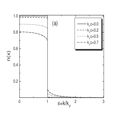
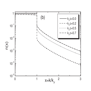
Figure 1: (a) The momentum distribution for correlated nuclear matter versus $k/k_{F}$ for various values of the correlation parameter $k_{F}c$ (b) The same, but on a logarithmic scale, for $n(x)$.

The behavior of the momentum distribution, as a function of $x=k/k_{F}$ for various values of the correlation parameter $k_{F}c$ is shown in Fig. 1. The discontinuity $Z$ is also displayed in each case. For ideal Fermi systems $Z=1$, while for interacting ones $Z<1$. In the limit of very strong interaction where $Z\rightarrow 0$, there is no discontinuity in the momentum distribution of the system. The quantity ($1-Z$) measures the ability of correlations to deplete the Fermi sea by exciting particles from states below it (hole states) to states above it (particle states) [61].

The asymptotic behavior of $n(1^{-})$ for $x->1^{-}$ reads [60]

$$n(1^{-})\approx 1-\frac{2}{3\pi^{2}}(\nu-1)(k_{F}c)^{2}\left[3\ln 2+1-3(x-1)\ln\mid x-1\mid+(6\ln 2-\frac{15}{2})(x-1)\right],$$ (11)

while for $x->1^{+}$

$$n(1^{+})\approx\frac{2}{3\pi^{2}}(\nu-1)(k_{F}c)^{2}\left[\frac{}{}3\ln 2-1-3(x-1)\ln(x-1)-(6\ln 2-7)(x-1)\right].$$ (12)

It is worthwhile to note the existence of a logarithmic singularity in the function $n(k)$ at $k=k_{F}$, a general feature of normal Fermi systems.

The discontinuity $Z$, according to Eqs (10) and (11), (12) is given by

$$Z=1-\frac{4}{\pi^{2}}\ln 2(\nu-1)(k_{F}c)^{2}.$$ (13)

The energy per particle $E$ of the ground state of $\nu=4$-component fermion fluid of hard-spheres, in the low-density expansion, has been derived in Refs. [62]. Accordingly, the energy $E$, in units of the ideal gas energy $E_{0}$, is given by [62]

$$E/E_{0}=e(y)\simeq 1+D_{1}y+D_{2}y^{2}+D_{3}y^{3}+D_{4}y^{4}\ln y,\qquad y=k_{F}c,\quad E_{0}=\frac{3}{5}\frac{\hbar^{2}k_{F}^{2}}{2m}.$$ (14)

where the coefficients $D_{i}$ are given in Table VI of Ref. [62]. It is one of the aims of the present work to investigate the connection between the various information measures and complexity with experimental quantities (as the ground state energy and the discontinuity $Z$). In addition, we intend to produce not only qualitative but mostly quantitative results, by connecting the strength of the correlations with the above measures.

2.2 Information measures

The information entropy in momentum space is given by the relation

$$S_{k}=-\int n(k)\ln{n(k)}\,\textrm{d}{\bf k}.$$ (15)

So, for an ideal Fermi gas, using Eq. (4), $S_{k}$ becomes

$$S_{k}=S_{0}=\ln V_{k}=\ln\left(\frac{6\pi^{2}}{\nu}\frac{1}{r_{0}^{3}}\right).$$ (16)

For correlated Fermi systems, $S_{k}$, can be found from Eq. (15) by employing Eq. (1). $S_{k}$ is written now [13]

$$S_{k}=\ln V_{k}-\frac{4\pi}{V_{k}}\left(\int_{0}^{k_{F}^{-}}k^{2}n_{<}(k)\ln n_{<}(k)dk+\int_{k_{F}^{+}}^{\infty}k^{2}n_{>}(k)\ln n_{>}(k)dk\right).$$ (17)

The correlated entropy $S_{k}$ has the form

$$S_{k}=S_{0}+S_{\rm cor},$$ (18)

where $S_{0}$ is the uncorrelated entropy given by Eq. (16) and $S_{\rm cor}$ is the contribution of the particle correlations to the entropy. That contribution can be found from the expression

$$S_{\rm cor}=-3\left(\int_{0}^{1^{-}}x^{2}n_{<}(x)\ln n_{<}(x)dx+\int_{1^{+}}^{\infty}x^{2}n_{>}(x)\ln n_{>}(x)dx\right),$$ (19)

where $x=k/k_{F}$.

The disequilibrium $D_{k}$ (or information energy, defined by Onicescu [17]), in momentum space as another functional of a probability distribution, in our case $n(k)$ is given by the relation

$$D_{k}=\int n^{2}(k)d{\bf k}.$$ (20)

For an ideal Fermi gas, using Eq. (4), becomes

$$D_{k}=D_{0}=\frac{1}{V_{k}}.$$ (21)

In the case of correlated Fermi systems, $D_{k}$ is written as

$$D_{k}=\frac{1}{V_{k}}\frac{4\pi}{V_{k}}\left(\int_{0}^{k_{F}^{-}}k^{2}n^{2}_{<}(k)dk+\int_{k_{F}^{+}}^{\infty}k^{2}n^{2}_{>}(k)dk\right).$$ (22)

The correlated disequilibrium $D_{k}$ is

$$D_{k}=D_{0}D_{\rm cor},$$ (23)

where $D_{0}$ is given in Eq. (21) and $D_{cor}$ can be found also from the expression

$$D_{cor}=3\left(\int_{0}^{1^{-}}x^{2}{n}^{2}_{<}(x)dx+\int_{1^{+}}^{\infty}x^{2}{n}^{2}_{>}(x)dx\right).$$ (24)

The statistical complexity measure, proposed by Catalan et. al. [34], in momentum space, is defined as

$$C_{\rm LMC}=C=D_{k}H_{k},$$ (25)

where $H$ represents the information content of the system defined as

$$H_{k}=\textrm{e}^{S_{k}}.$$ (26)

It is easy to show that

$$C=C_{0}C_{\rm cor}=D_{\rm cor}\textrm{e}^{S_{\rm cor}},\qquad C_{0}=D_{0}\textrm{e}^{S_{0}}=1.$$ (27)

The physical meaning of Eq. (27) is clear. In the case of an ideal Fermi gas (see Eq. (4)) $C$ is minimal with the value $C_{0}=1$ (see also [34]). Moreover as pointed out in Ref. [34], $C$ is not an upper bounded function and can therefore become infinitely large. From the above analysis it is clear that complexity $C$ is an accounter of correlations in an infinite Fermi system. Thus, the next step is to try to find the connection between $C$ and the correlation parameters of the systems. The correlation invoke diffusion of the momentum distribution and we expect this effect to be reflected on the values of $C$.

3 Results and discussion

The behavior of the momentum distribution, as a function of $k/k_{F}$, for various values of the wound parameter $k_{F}c$ is shown in Fig. 1. The discontinuity $Z$ is also displayed in each case. For ideal Fermi systems $Z=1$, while for interacting ones $Z<1$. In the limit of very strong interaction $Z=0$, there is no discontinuity on the momentum distribution of the system.

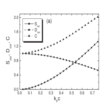
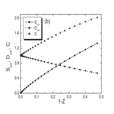
Figure 2: (a) $S_{cor}$, $D_{cor}$ and $C$ of nuclear matter versus the the correlation parameter $k_{F}c$ and (b) the discontinuity parameter $(1-Z)$

The calculated values of $S_{\rm cor}$, $D_{\rm cor}$ and $C$ for nuclear matter versus the correlation parameter $k_{F}c$ are displayed in Fig. 2. $S_{\rm cor}$ and $C$ increase with $y$, while $D_{\rm cor}$ decreases. We fitted the numerical values of the above quantities, with simple functions of $y=k_{F}c$ and we find respectively the following formulae

$$S_{\rm cor}(y)=\alpha y^{\beta},\qquad\alpha=2.16379,\quad\beta=1.67053.$$ (28)

$$D_{\rm cor}(y)=1+\alpha y^{\beta},\qquad\alpha=-0.79871,\quad\beta=1.83155.$$ (29)

$$C(y)=1+\alpha y^{\beta},\qquad\alpha=1.68358,\quad\beta=1.67566.$$ (30)

The values of the parameters $\alpha$, $\beta$ and $\gamma$, for each case, have been selected by a least squares fit (LSF) method. It is worthwhile to notice that for an ideal Fermi gas there is an upper limit for $C$ ($C_{max}\simeq 1.5845$) [56]. However, for an interacting Fermi gas there is no such constraint (at least to the region under consideration in the present work). It is obvious that the calculated values of complexity reflect the different way that the interaction or temperature affect the trend of the momentum distribution.

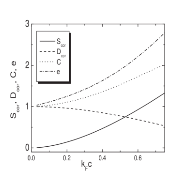
Figure 3: $S_{cor}$, $D_{cor}$, $C$ and the energy fraction $e$ (for definition see Eq. (14)) versus the correlation parameter $k_{F}c$.

The quantity ($1-Z$) measures the ability of correlations to deplete the Fermi sea by exciting particles from states below it (hole states) to states above it (particle states) [61]. The dependence of $S_{\rm cor}$, $D_{\rm cor}$ and $C$ on the quantity $(1-Z)$ is shown in Fig. 3. It is seen that $S_{\rm cor}$ and $C$ are increasing functions of $(1-Z)$, while $D_{\rm cor}$ is a decreasing one, as a direct consequence of the dependence of the above quantities on the correlation parameter $k_{F}c$. That dependence can be reproduced very well by simple expressions as in Eqs. (28), (29) and (30) replacing $k_{F}c$ by $(1-Z)$

$$S_{\rm cor}(Z)=\alpha(1-Z)^{\beta},\qquad\alpha=2.49614,\quad\beta=0.83527.$$ (31)

$$D_{\rm cor}(Z)=1+\alpha(1-Z)^{\beta},\qquad\alpha=-0.93413,\quad\beta=0.91574.$$ (32)

$$C(Z)=1+\alpha(1-Z)^{\beta},\qquad\alpha=1.94305,\quad\beta=0.83784.$$ (33)

From the above analysis we can conclude that LMC complexity $C$ can be employed as a measure of the strength of correlations in the same way the wound and the discontinuity parameters are used. An explanation of the above behavior of $C$ is the following: The effect of nucleon correlations is the departure from the step function form of the momentum distribution (ideal Fermi gas) to the one with long tail behavior for $k>k_{F}$. The diffusion of the distribution leads to a decrease of the order of the system (the disequilibrium $D_{k}$ decreases and the information entropy $S_{k}$ increases accordingly). In total, the contribution of $S_{k}$ in $C$ dominates over the contribution of $D_{k}$ and thus the complexity increases with the correlations (at least in the region under consideration).

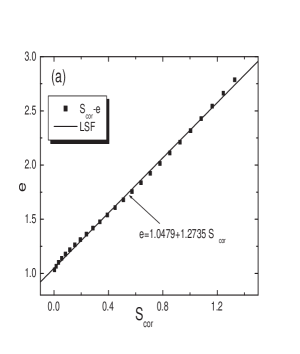
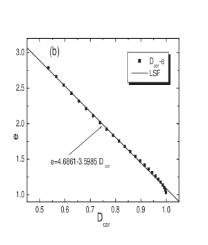
Figure 4: The energy fraction $e$ versus (a) $S_{cor}$ (b) $D_{cor}$ and (c) $C$. The lines corresponds to the expressions (34), (35) and (36), respectively with the parameters derived by the least squares fit method (LSF).

It is one of the aims of the present work to connect $C$, a measure of complexity based on a probabilistic description and the shape of the corresponding momentum distributions with other quantities like the ground state energy per particle $E$. In view of the above, we display in Fig. 3 the dependence of $S_{cor}$, $D_{cor}$ and $C$, as well as the energy fraction $e(y)$, on the correlation parameter $k_{F}c$. The dependence of $S_{cor}$, $D_{cor}$ and $C$ on $e(y)$, as displayed in Fig. 4, is in a very good approximation linear. The fitted expressions are the following:

$${\rm e}=1.0479+1.27353S_{cor},$$ (34)

$${\rm e}=4.6861-3.5985D_{cor},$$ (35)

$${\rm e}=-0.5847+1.6358C.$$ (36)

In total we observe an empirical connection of the energy with $S_{cor}$, $D_{cor}$ and $C$ calculated employing information entropy, which, by definition, is not related directly to the energy of the system, in contrast to the traditional concept of thermodynamic entropy. The above results confirm our recent finding, according to similar lines, that there is also a connection between the ”energy-like” quantity specific heat $C_{V}$ of an ideal electron gas with the complexity $C$ [56].

Finally, in Fig. 5 we compare the present results with those taken from the Low Order Approximation (LOA) method. Thus the momentum distribution of nuclear matter is evaluated by employing the LOA and the MD takes the form [61]

$$n_{\rm LOA}(k)=\theta(k_{F}-k)\left[1-k_{\rm dir}+Y(k,8)\right]+8\left[k_{\rm dir}Y(k,2)-[Y(k,4)]^{2}\right],$$ (37)

where

$$c_{\mu}^{-1}Y(k,\mu)=\frac{\textrm{e}^{-\tilde{k}_{+}^{2}}-\textrm{e}^{-\tilde{k}_{-}^{2}}}{2\tilde{k}}+\int_{0}^{\tilde{k}_{+}}\textrm{e}^{-y^{2}}\,\textrm{d}y+{\rm sgn}(\tilde{k}_{-})\int_{0}^{\mid\tilde{k}_{-}\mid}\textrm{e}^{-y^{2}}\textrm{d}y,$$ (38)

and

$$c_{\mu}=\frac{1}{8\sqrt{\pi}}\left(\frac{\mu}{2}\right)^{3/2},\quad\tilde{k}=\frac{k}{\beta\sqrt{\mu}},\quad\tilde{k}_{\pm}=\frac{k_{F}\pm k}{\beta\sqrt{\mu}},\quad\mu=2,4,8.$$ (39)

while ${\rm sgn}(x)=x/\mid x\mid$. The dimensionless wound parameter $k_{\rm dir}$ can serve as a rough measure of correlations and the rate of convergence of the cluster expansion is defined as

$$k_{\rm dir}=\rho\int[f(r)-1]^{2}\,\textrm{d}{\bf r}.$$ (40)

The normalization condition for the momentum distribution is

$$\int_{0}^{\infty}n_{\rm LOA}(k)k^{2}\textrm{d}k=\frac{1}{3}\,k_{F}^{3}.$$ (41)

The following relation between the wound parameter $k_{\rm dir}$ and the correlation parameter $\beta$

$$k_{\rm dir}=\frac{1}{3\sqrt{2\pi}}\left(\frac{k_{F}}{\beta}\right)^{3}.$$ (42)

It is clear that large values of $k_{\rm dir}$ imply strong correlations and simultaneously poor convergence of the cluster expansion. In the numerical calculations the correlation parameter $\beta$ is in the interval: $1.01\leq\beta\leq 2.482$. That range corresponds to $0.3\geq k_{\rm dir}\geq 0.02$ and this is reasonable, in the case of nuclear matter [61]. However, the origin of the two methods is different and as a consequence they influence in a different way the momentum distribution. Nevertheless, we found that $S_{cor}$, $D_{cor}$ and $C$ exhibit a similar trend as a functions of the parameter $1-Z$.

4 Conlusions

In conclusion, we calculate information and complexity measures of a uniform Fermi system, like nuclear matter, in the framework of the hard-sphere model. The effect of correlations is connected intuitively with the concept of complexity, in a qualitative, and somehow vague way as stated in [56] as well. In fact, it turns out that all information measures used by us, show a strong dependence on the correlation parameter $k_{F}c$ as well as on the Fermi discontinuity $Z$. The most distinctive feature is the occurrence of an almost linear dependence between information measures and complexity on energy. The above statement is in keeping with the recent finding of the existence of an empirical connection between the specific heat and complexity [56]. However, the applicability of our approach is much wider than nuclear matter, since the impenetrable hard spheres (not overlapping in space) can simulate the extremely strong repulsion that atoms and spherical molecules feel at very small distances. Thus, the significance of a suitable quantification of complexity emerges in statistical mechanics of fluids and solids. We do not claim that our approach is the only or more important one, but so far our results are interesting and encouraging. We stress again that the proposed LMC measure of complexity is by its definition an appropriate one and specifically tailored for systems described statistically, through a probability distribution. Since ”information is physical” [63], it is promising to examine how far this quotation goes, in the sense that calculations employing a good measure of information content of a quantum system (and consequently of complexity) are expected to give, at least, interesting results of physical relevance. Landauer dedicated his research on similar ideas. Hence, in our present work and previous ones, we proceed towards a numerical quantification of complexity. One of our goals is to examine, as a first step, whether a particular definition of complexity is reasonable and robust enough e.g. if one increases the value of one parameter (or parameters) describing a quantum system, the corresponding value of complexity increases accordingly. This would satisfy minimally intuition about complexity and validate its definition.

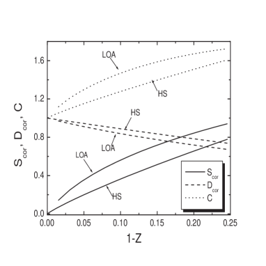
Figure 5: $S_{cor}$, $D_{cor}$ and $C$ of nuclear matter versus the the discontinuity parameter $(1-Z)$ calculated by employing two different methods: the Low Order Approximation (LOA) (see text) and the hard sphere interaction (HS).

References

- [1] G.A. Cowan, D. Pines, and D. Meltzer, Complexity: Metaphors, Models and Reality, (Addison-Wesley, Redwood City, 1999).
- [2] I. Bialynicki-Birula and J. Mycielski, Commun. Math. Phys. 44, (1975) 129.
- [3] S.B. Sears, Applications of information theory in chemical physics, Ph.D. Thesis, Univiversity of North Caroline at Chapel Hill (1980).
- [4] C. Adami, Information theory in molecular bilogy, Phys. of Life Reviews, 1 (2004).
- [5] A. Borst and F.E. Theunissen, Nature Neuroscience 2, 947 (1999).
- [6] T.M. Cover and J.A. Thomas, Element of Information Theory Wiley Series in Telecommunitions.
- [7] M.A. Nillsen and I.L. Chuang, Quantum Computation and Quantum Informtion Cambridge University Press.
- [8] K.Ch. Chatzisavvas, Ch.C. Moustakidis, and C.P. Panos, J. Chem. Phys. 123, 174111 (2005).
- [9] K.D. Sen, C.P. Panos, K.Ch. Chatzisavvas, and Ch.C. Moustakidis, Phys. Lett. A 364, 286 (2007).
- [10] C.P. Panos, K.Ch. Chatzisavvas, Ch.C. Moustakidis, and E.G. Kyrkou, Phys. Lett. A 363, 78 (2007).
- [11] C.P. Panos and S.E. Massen, Int.J. Mod. Phys. E 6, 497 (1997); G.A. Lalazissis, S.E. Massen, C.P. Panos, and S.S. Dimitrova, Int. J. Mod. Phys. E 7, 485 (1998).
- [12] S.E. Massen and C.P. Panos, Phys. Lett. A 246, 530 (1998); S.E. Massen and C.P. Panos, Phys. Lett. A 280, 65 (2001); S.E. Massen, Ch.C. Moustakidis, and C.P. Panos, Phys. Lett A 299, 131 (2002); C.P. Panos, Phys. Lett. A 289, 287 (2001).
- [13] Ch.C. Moustakidis and S.E. Massen, Phys. Rev. B 71, 045102 (2005).
- [14] K.Ch. Chatzisavvas and C.P. Panos, Int. J. Mod. Phys. E, 14, 653 (2005).
- [15] C.E. Shannon, Bell Syst. Tech. J. 27, 379 (1948).
- [16] R.A. Fisher, Proc. Cambridge Phil. Sec. 22, 700 (1925).
- [17] O. Onicescu, Theorie de l information. Energie informationelle., Vol. 263 of A, C. R. Acad. Sci. Paris, 1966.
- [18] S. Kullback, Statistics and Information theory, (Wiley, New York, 1959).
- [19] A. Rényi On measures of information and entropy, Proceedings of the 4th Berkeley Symposium on Mathematics, Statistics and Probability 1960, pp. 547-561 (1961).
- [20] S.R. Gadre, Phys. Rev. A 30, 620 (1984); S.R. Gadre, S.B. Sears, S.J. Chakravorty, and R.D. Bendale, Phys. Rev. A 32, 2602 (1985); S.R. Gadre and R.D. Bendale, Phys. Rev. A 36, 1932 (1987).
- [21] M. Ohya and P. Petz, ”Quantum entropy and its use” (Springer Berlin, 1993).
- [22] V. Zelevinsky, M. Horoi, and B.A. Brown, Phys. Lett. B 350, 141 (1995). V.V. Sokolov, B.A. Brown, and V. Zelevinsky, Phys. Rev E 58, 56 (1998).
- [23] A. Nagy and R.G. Parr, Int. J. Quant. Chem. 58, 323 (1996).
- [24] V. Majernic and T. Opatrny, J. Phys. A 29, 2187 (1996).
- [25] S.K. Ghosh, M. Berkowitz, and R.G. Parr, Proc. Natl. Acad. Sc. USA 81, 8028 (1984).
- [26] P. Garbaczewski, J. Stat. Phys. 123, 315 (2006).
- [27] B.R. Frieden, Science from Fisher Information, (Cambridge University Press, 2004).
- [28] S.H. Patil, K.D. Sen, N.A. Watson, and H.E. Montogomery, J. Phys. B 40, 2147 (2007).
- [29] S.B. Liu, J. Chem. Phys. 126, 191107 (2007).
- [30] A.V. Luzanov and O.V. Prezhdo, Mol. Phys. 105, 2879 (2007).
- [31] J. Antolín and J.C. Angulo, Eur. Phys. J. D 46, 21 (2008).
- [32] R.P. Sagar and N.L. Guevara, J. Mol. Struct. (Theochem) 857, 72 (2008).
- [33] R. López-Ruiz, H.L. Mancini, and X. Calbet, Phys. Lett. A 209, 321 (1995).
- [34] R.G. Catalán, J. Garay, and R. López-Ruiz, Phys. Rev. E 66, 011102 (2002).
- [35] J. Sañudo and A.F. Pacheco, Phys. Lett. A 373, 807 (2009).
- [36] P.T. Landsberg and J.S. Shiner, Phys. Lett. A 245, 228 (1998); P.T. Landsberg, Phys. Lett. A 102, 171 (1984).
- [37] J.S. Shiner, M. Davison, and P.T. Landsberg, Phys. Rev. E 59, 1459 (1999).
- [38] D.P. Feldman and J.P. Crutchfield, Phys. Lett. A 238, 244 (1998).
- [39] J.P. Crutchfield, D.P. Feldman, and C.R. Shalizi, Phys. Rev. E 62, 2996 (2000).
- [40] P.M. Binder and N. Perry, Phys. Rev. E 62, 2998 (2000).
- [41] M.T. Martin, A. Plastino, and O.A. Rosso, Phys. Lett. A 311, 126 (2003).
- [42] C.P. Panos, N.S. Nikolaidis, K.Ch. Chatzisavvas, and C.C. Tsouros, Phys. Lett. A 373, 2343 (2009).
- [43] R. López-Ruiz, Biophys. Chem. 115, 215 (2005).
- [44] T. Yamano, J. Math. Phys. 45, 1974 (2004).
- [45] C. Anteneodo and and A.R. Plastino, Phys. Lett. A 223, 348 (1996).
- [46] A. Borgoo, F. De Proft, P. Geerlings, and K.D. Sen, Chem. Phys. Lett. 444, 186 (2007).
- [47] H.E. Montgomery and K.D. Sen, Phys. Lett. A 372, 2271 (2008).
- [48] X. Calbet and R. López-Ruiz, Physica A 382, 523 (2007).
- [49] J.C. Angulo and J. Antolín, J. Chem. Phys. 128, 164109 (2008).
- [50] J.C. Angulo, J. Antolín, and K.D. Sen, Phys. Lett. A 372, 670 (2008).
- [51] J. Sañudo and R. López-Ruiz, Phys. Lett. A 372, 5283 (2008).
- [52] J. Sañudo and R. López-Ruiz, J. Phys. A 41, 265303 (2008).
- [53] K.Ch. Chatzisavvas, V.P. Psonis, C.P. Panos, and Ch.C. Moustakidis, Phys. Lett. A 373, 3901 (2009).
- [54] S. López-Rosa, D. Manzano, and J.S. Dehesa, Physica A 388, 3273 (2009).
- [55] R. López-Ruiz, A. Nagy, E. Romera, and J. Sañudo, Journ. of Mathem Phys. 50, 123528 (2009).
- [56] Ch.C. Moustakidis, V.P. Psonis, K.Ch. Chatzisavvas, C.P. Panos, and S.E. Massen, Phys. Rev. E 81, 011104 (2010).
- [57] J. Antolín, S. Lopéz-Rosa, J.C. Angulo, Chem. Phys. Lett. 474 233 (2009).
- [58] A.N. Kolmogorov, Probl. Inf. Transm. 1, 3 (1965).
- [59] W. Czyż and K. Gottfried, Nucl. Phys. 21, 676 (1961).
- [60] R. Sartor and C. Mahaux, Phys. Rev. C 21, 1546 (1980); R. Sartor and C. Mahaux, Phys. Rev. C 25, 677 (1982).
- [61] M.F. Flynn, J.W. Clark, R.M. Panoff, O. Bohigas, and S. Stringari, Nucl. Phys. A427, 253 (1984).
- [62] G.A. Baker Jr., L.P. Benofy, M. Fortes, M. de Llano, S.M. Peltier and A. Plastino, Phys. Rev. A 26, 3575 (1982); G.A. Baker Jr., G. Gutierrez, and M.de Llano, Ann. of. Phys. 153, 283 (1984); M.A. Solis, M. De Llano, J.W. Clark, and G.A. Baker Jr., Phys. Rev. E 76, 031125 (2007).
- [63] D.P. Di Vincenzo and D. Loss, Quantum Information is Physical ArXiV: cond-mat/9710259.