Trapping Solids at the Inner Edge of the Dead Zone: 3-D Global MHD Simulations

Abstract

Context. The poorly-ionized interior of the protoplanetary disk or ‘dead zone’ is the location where dust coagulation processes may be most efficient. However even here, planetesimal formation may be limited by the loss of solid material through radial drift, and by collisional fragmentation of the particles. Both depend on the turbulent properties of the gas.

Aims. Our aim here is to investigate the possibility that solid particles are trapped at local pressure maxima in the dynamically evolving disk. We perform the first 3-D global non-ideal magnetohydrodynamical (MHD) calculations of a section of the disk treating the turbulence driven by the magneto-rotational instability (MRI).

Methods. We use the ZeusMP code with a fixed Ohmic resistivity distribution. The domain contains an inner MRI-active region near the young star and an outer midplane dead zone, with the transition between the two modeled by a sharp increase in the magnetic diffusivity.

Results. The azimuthal magnetic fields generated in the active zone oscillate over time, changing sign about every 150 years. We thus observe the radial structure of the ‘butterfly pattern’ seen previously in local shearing-box simulations. The mean magnetic field diffuses from the active zone into the dead zone, where the Reynolds stress nevertheless dominates, giving a residual $\alpha$ between $10^{-4}$ and $10^{-3}$. The greater total accretion stress in the active zone leads to a net reduction in the surface density, so that after 800 years an approximate steady state is reached in which a local radial maximum in the midplane pressure lies near the transition radius. We also observe the formation of density ridges within the active zone.

Conclusions. The dead zone in our models possesses a mean magnetic field, significant Reynolds stresses and a steady local pressure maximum at the inner edge, where the outward migration of planetary embryos and the efficient trapping of solid material are possible.

1 Introduction

Forming planets in a protoplanetary disk with a power-law surface density profile is difficult for several reasons. First, solid material on accumulating into meter-sized boulders quickly spirals to the star, transferring its orbital angular momentum to the gas (Weidenschilling, 1977; Nakagawa et al., 1986; Takeuchi & Lin, 2002; Youdin & Chiang, 2004; Brauer et al., 2007). Second, collisions between the constituents lead to disruption rather than growth when rather low speed thresholds are reached (Blum et al., 1998; Poppe et al., 1999; Blum & Wurm, 2000). Bodies in the meter size range are destroyed in impacts as slow as some cm/s (Benz, 2000). Turbulence in the gas readily yields collisions fast enough to terminate growth (Brauer et al., 2008a). Third, Earth-mass protoplanetary cores are prone to radial migration resulting from the tidal interaction with the gas, and in the classical type I migration picture quickly migrate all the way to the host star (Goldreich & Tremaine, 1980; Ward, 1986).

All three of these problems could be solved by the presence of local radial gas pressure maxima, which trap the drifting particles (Haghighipour & Boss, 2003), leading to locally enhanced number densities and high rates of low-speed collision (Lyra et al., 2008; Brauer et al., 2008b; Kretke et al., 2009). With sufficient local enhancement, one can envision the direct formation of planetesimals via collapse under the self-gravity of the particle cloud, bypassing the size regime most susceptible to the radial drift. Furthermore, the radial migration of Earth-mass protoplanets can be slowed or stopped by varying the surface density and temperature gradients (Masset et al., 2006). Migration substantially slower than in the classical picture appears to be required to explain the observed exoplanet population under the sequential planet formation scenario (Schlaufman et al., 2009).

The formation of local pressure maxima is governed by the radial transport of gas within the disk. The magneto-rotational instability or MRI (Balbus & Hawley, 1991, 1998) is currently the best studied candidate to drive such flows. Local shearing-box calculations show that the instability leads to long-lasting turbulence and to angular momentum transfer by magnetic forces, provided the magnetic fields are well-coupled to the gas (Hawley et al., 1995; Brandenburg et al., 1995; Sano et al., 2004; Johansen et al., 2009). Global ideal MHD calculations have been performed in various astrophysical contexts: protoplanetary disks (Steinacker & Henning, 2001; Arlt & Rüdiger, 2001; Fromang, 2005; Fromang & Nelson, 2006, 2009), black hole accretion toruses (Hawley, 2000), and galactic disks (Dziourkevitch et al., 2004). All the global simulations included neither a physical magnetic diffusivity nor a physical viscosity. Meanwhile, from local shearing-box studies it is known that the strength of the saturated MRI turbulence depends critically on the resistivity and viscosity (Lesur & Longaretti, 2007; Fromang & Papaloizou, 2007; Fromang et al., 2007). In particular, whereas the molecular viscosity is small in protostellar disks, the gas is so weakly ionized in the cold disk interior (Gammie, 1996; Igea & Glassgold, 1999; Semenov et al., 2004) that the Ohmic resistivity shuts down the linear MRI and prevents the development of turbulence (Sano et al., 1998; Sano & Stone, 2002a, b; Fleming & Stone, 2003; Turner et al., 2007).

In this paper we present the first global resistive MHD calculations to include the ‘dead zone’ where the rapid diffusion of the magnetic fields prevents magnetorotational turbulence. Local pressure maxima form in the calculations in two ways: at dead zone edges and in zonal flows. The dead zone edges yield long-lived rings of enhanced surface density near locations where a gradient in the ionization fraction leads to a jump in the accretion stress (Kretke & Lin, 2007). The zonal flows on the other hand result from local fluctuations in the Maxwell stress in the turbulence, and lead to pressure maxima with lifetimes of a few orbits (Johansen et al., 2009).

In the next section we describe our disk model and the choice of magnetic resistivity profiles. The third section presents the results, starting from the global properties of the magnetic field, followed by the effects of the resistivity jump on the surface density. In the fourth section we discuss the interaction of the magnetic fields with the density rings and with radial minima appearing in the turbulent activity. Our main results are summarized in section 5.

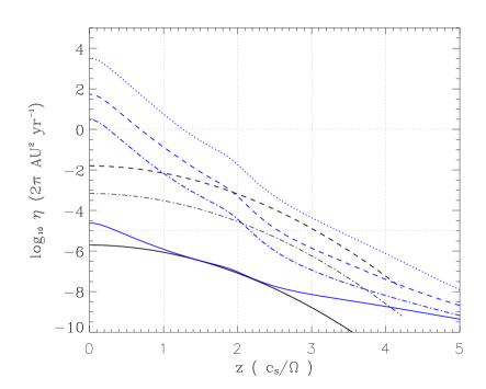
Figure 1: Vertical profiles of magnetic diffusivity. Black lines show the profiles adopted for simulations of the dead zone, with $\eta_{0}=2\cdot{}10^{-6}$ (solid), $\eta_{0}=7\cdot{}10^{-4}$ (dot-dashed) and $\eta_{0}=0.016$ (dashed) (see Eq. 6). Blue lines show the estimations of magnetic diffusivity made for the disk at 4.5 AU using the simple gas-phase reaction set (Oppenheimer & Dalgarno, 1974; Ilgner & Nelson, 2006) together with dust grains. The solid line is for no grains, dotted for $0.1{\rm\mu m}$, dashed for $1{\rm\mu m}$ and dot-dashed for $10{\rm\mu m}$ dust grains.

2 Model Description

The initial setup for the models is very similar to those studied by Fromang & Nelson (2006) for the ideal MHD case. In our models, MRI-driven turbulence is operating in locally-isothermal disk, with a fixed spatial distribution for the temperature. To describe the dead zone in the protoplanetary disk, we include the Ohmic dissipation in our models. The Ohmic dissipation is the largest non-ideal term in the induction equation under typical dusty conditions (Wardle, 2007). Ambipolar diffusion and Hall effect are not considered for the sake of simplicity. The vertical profile of magnetic diffusivity (see section 2.1) is adopted from separate chemistry calcullations and is fixed in space and time.

We solve the set of MHD equations using 3D global simulations on a spherical grid $(r,\Theta,\phi)$,

$$\frac{\partial\mbox{\boldmath$B$}}{\partial t}=\nabla\times[\mbox{\boldmath$u$}\times\mbox{\boldmath$B$}-\eta(\Theta)\nabla\times\mbox{\boldmath$B$}],$$ (1)

$$\frac{\partial\mbox{\boldmath$u$}}{\partial t}=-\frac{1}{\rho}\nabla P+\nabla\Psi+\frac{1}{4\pi\rho}[\nabla\times\mbox{\boldmath$B$}]\times\mbox{\boldmath$B$},$$ (2)

$$\frac{\partial\rho}{\partial t}+\nabla\cdot(\rho\mbox{\boldmath$u$})=0.$$ (3)

The notation is the usual one. $\Psi$ is a point-mass gravitational potential and $\sqrt{G{M}_{\star}}$ is set to unity in the code units. We use the locally isothermal approach to describe vertically stratified disks, adopting $P=c_{\rm s}^{2}(r)\rho(r,\Theta)$ with a sound speed $c_{\rm s}=c_{0}/(r\cdot{}\sin(\Theta))$ and $H/R=0.07$. The initial field setup is exactly the equilibrium solution,

$$u_{\phi}=\frac{1}{r}\sqrt{1-\frac{c_{0}^{2}(1+a)}{\sin{\Theta}}},$$ (4)

$$\rho=\rho_{0}\frac{1}{(r\sin{\Theta})^{a}}\exp{\left(-\frac{\cos{\Theta}^{2}}{2c_{0}^{2}\sin{\Theta}^{2}}\right)},$$ (5)

where $a=3/2$.

We consider the inner part of the protoplanetary disk, which is heavier and warmer compared to a minimum solar-nebula. In order to mimic a ’dead zone’ and the ionization thresholds, we adopt fixed magnetic diffusivity profiles $\eta(\Theta)$. We use the estimations from dynamical disk chemistry simulations for the adopted disk parameters $\Sigma,T$ (Turner et al., 2007). The surface density is $\Sigma=(R/3.75{\rm AU})^{-1/2}\cdot 1700\ \rm g/cm^{2}$, and the temperature is $T=(R/3.75{\rm AU})^{-1}\cdot 280\rm K$, where $R$ is cylinder radius. The units are $[u_{\phi}]=2\pi\ {\rm AU/yr}=29.8\ {\rm km/s}$ for velocity and $[\eta]=2\pi\ {\rm AU^{2}/yr}=4.47\cdot{}10^{19}\ {\rm cm^{2}/s}$ for magnetic diffusivity. The models are listed in Table 1.

Our models include the disk part from 2 to 10 AU. A purely azimuthal magnetic field is chosen as seed field for MRI turbulence, which is $P_{\rm gas}/P_{\rm mag}=25$ everywhere in the disk. The Alfvén limiter of $c_{\rm lim}=14c_{0}$ is applied. We use reflective radial boundary condition, with buffer zones applied at radii $2{\rm AU}<r<2.5{\rm AU}$ and $9.5{\rm AU}<r<10{\rm AU}$. We apply the magnetic diffusivity within the buffer zones: $\eta_{\rm buffer}$ is $10^{-5}$ at the radial boundary and decreases linearly towards the physical domain. The buffer zones have both damping of radial velocity towards zero at the border, and diffusing away the magnetic eddies approaching the radial boundary.

Periodic boundary conditions are applied both for azimuthal and vertical (i.e. $\Theta$) domain borders.

Table 1: Model properties and midplane $\alpha$-stresses inside ($\alpha_{\rm A}$) and outside ($\alpha_{\rm D}$) of the ionization threshold radius $r_{\rm th}$

Model	Resolution	$r_{\rm th}$[AU]	$\eta_{\rm A}$	$\eta_{\rm D}$	$\alpha_{\rm A}$	$\alpha_{\rm D}$	Time [years]
$\rm M_{IR}$	[256:128:64]	4.5	$2.10^{-6}$	$7.10^{-4}$	$1.9\cdot{}10^{-3}$	$1.0\cdot{}10^{-3}$	880
$\rm M_{IR/2}$	[128:64:32]	4.5	$2.10^{-6}$	$7.10^{-4}$	$1.3\cdot{}10^{-3}$	$2.1\cdot{}10^{-4}$	960
$\rm M_{ID}$	[256:128:64]	4.5	$2.10^{-6}$	$0.016$	$1.6\cdot{}10^{-3}$	$2.9\cdot{}10^{-4}$	650
$\rm M_{IR6}$	[256:128:64]	6.5	$2.10^{-6}$	$7.10^{-4}$	$2.9\cdot{}10^{-3}$	$1.6\cdot{}10^{-3}$	1100
$\rm M_{\rm ideal}$	[256:128:64]	none	$2.10^{-6}$	$2.10^{-6}$	$5.4\cdot{}10^{-3}$	$5.4\cdot{}10^{-3}$	682 $*$

2.1 Ionization Thresholds and Influence of Dust Grains

An estimate of the magnetic diffusivity vs. height at 4.5 AU is shown in Fig. 1. The midplane diffusivity with dust grains appears to be substantially higher then it is possible to include in the MHD simulations. The four blue curves from top to bottom are demonstrating the magnetic diffusivity in code units for the gas and dust grains of 0.1, 1 and 10 microns, and no grains. We have used the simple gas-phase reaction set of Oppenheimer & Dalgarno (1974) together with the grain surface chemistry of Ilgner & Nelson (2006) for the classical dust to gas ratio. Ionization by stellar X-rays, cosmic rays and long-lived radionuclides is included. The penetration depths are assumed $8\rm g/cm^{2}$ for the X-rays and $96$ for the cosmic rays.

The exact calculations of chemistry and dust behavior in the thermally evolving global disk is a hard task with many free parameters. After planetesimals form, the dust mass fraction will be lower than the interstellar value. We shall bear in mind that CRP stopping depth can be as low as $36\rm g/cm^{2}$ (Glassgold et al., 2009).

Here we simplify the situation and adopt the following time-independent vertical profile of magnetic diffusivity,

$$\eta=\eta_{0}\exp{\left(\frac{\sin{\Theta}-1}{c_{0}^{2}}\right)^{1.55}},$$ (6)

where $\eta_{0}$ is the midplane value of magnetic diffusivity. In Fig. 1, black lines show the profiles adopted for our simulations, with $\eta_{0}=2\cdot{}10^{-6}$ (solid), $\eta_{0}=7\cdot{}10^{-4}$ (dot-dashed) and $\eta_{0}=0.016$ (dashed). To simulate the situation mentioned in Kretke & Lin (2007); Kretke et al. (2008), we drop the radial dependence of $\eta$ and suggest that $\eta_{0}$ makes the jump at the chosen threshold radius $r_{\rm th}$. For example, in model $\rm M_{IR}$ (section 2.2, Table 1), the Ohmic diffusion is following a black solid line in Fig. 1 for radii from 2 to 4.5 AU, and a dot-dashed line for radii from 4.5 to 10 AU. The magnetic diffusivity in the disk without dust grains is low, so that we have MRI-active region from 2 to 4.5 AU. The dead zone begins where the dust grains are present. The exact location of the inner edge of the dead zone (i.e. $r_{\rm th}$) depends on the properties of the star and the dust in the disk, and can vary from object to object. Our choice for locating the threshold $r_{\rm th}$ is quite arbitrary. We place $r_{\rm th}$ roughly in the middle of our inner global disk patch (Table 1).

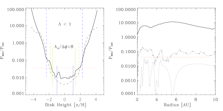
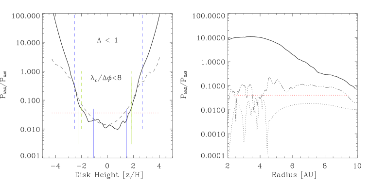
Figure 2: Inverse plasma $\beta$. Top: model $\rm M_{IR}$ at $t=300$ years; Below: $\rm M_{IR/2}$ (halved space resolution) at the same time. Left: The change of inverse plasma $\beta$ vertical distribution from initial (red) to the convex shape (black lines). The solid line stands for inverse plasma beta averaged within active zone ($2.5\to 4.5$ AU). Dashed line is for the $1/\beta$ averaged over the patch of the dead zone ($5\to 7$AU). Vertical bars mark the disk height where the Elsässer number drops below unity (blue lines, solid for active and dashed for dead zones). Green lines border the midplane region with $\lambda_{\rm c}/\Delta\phi<8$ (Eq. 11). Right: Radial dependence of vertically averaged $1/\beta$ (solid line), $1/\beta$ at the midplane (dotted line) and at $z=2H$ (dashed line).

2.2 Set of Simulations

Models in Table 1 have an ionization threshold posed either at $4.5\rm AU$ or $6.5\rm AU$. Midplane values for magnetic diffusivity are noted in Table 1 as $\eta_{\rm A}$ and $\eta_{\rm D}$ (‘Active’ and ‘Dead’) for gas states inside and outside the threshold radius. The time duration of each model is given in years, and the mark $*$ is given when the steady-state has not been reached. Vertical profiles for magnetic diffusivity follow Eq. 6 and are demonstrated in Fig. 1 with black lines. Each model combines two diffusivity profiles, except the run $\rm M_{IDEAL}$.

In Table 1, notations are ’I’ for quasi-ideal MHD state with $\eta_{0}=2\cdot{}10^{-6}$ (Fig. 1, solid black line), ’R’ for the gas disk with $10{\rm\mu m}$-sized dust grains ($\eta_{0}=7\cdot{}10^{-4}$, dot-dashed black line), ’D’ for the case of $1\rm\mu m$ grains ($\eta_{0}=0.016$, dashed black line). Our adopted magnetic diffusivity profiles for the disk with $1\rm\mu m$ and $10{\rm\mu m}$-sized dust grains will allow the turbulent MRI layers beyond $3$H and $2$H, correspondingly. The peak values of blue curves in Fig. 1 are leading to unacceptable short time steps in resistive MHD simulations. We have observed that it is not convenient to compute the regions with $\eta>0.1\rm AU^{2}/yr$ with standard MHD codes, because of the dramatic shortening of the time step. For this numerical reason, we take the magnetic diffusivity slightly different as the chemistry models predict. Our adopted profiles of magnetic diffusivity (black curves, Fig. 1) allow to match the values of chemical models at 2 AU and remain above the numerical dissipation for region between 2H and 3H. Reducing of the magnetic diffusivity in the dead zone may influence how fast the global magnetic fields are diffused into the dead zone, whereas the MRI modes are damped all the same.

2.3 Calculation of Turbulent Stresses

An important outcome of our simulations is the magnitude of the Reynolds and Maxwell stresses. To calculate the latter, we use the approach described in Fromang & Nelson (2006) for curvi-linear coordinates. The turbulent viscosity can be described as $\nu=\alpha c_{\rm s}^{2}/\Omega$, where the main component of the $\alpha$ stress tensor is

$$\alpha_{r,\phi}=\frac{T_{\rm M}+T_{\rm R}}{\langle{P\rangle}},$$ (7)

or $\alpha=\alpha_{\rm R}+\alpha_{\rm M}$. The Reynolds and Maxwell stresses are calculated as

$$T_{\rm R}=\langle{(\rho u_{\phi}^{{}^{\prime}}u_{r}^{{}^{\prime}})\rangle},$$ (8)

$$T_{\rm M}=-\langle{(B_{\phi}^{{}^{\prime}}B_{r}^{{}^{\prime}})/4\pi\rangle},$$ (9)

The mean pressure for azimuthal domain $\Delta\phi$ is

$${\langle{P(r)\rangle}}=c_{\rm s}(r)^{2}\Sigma(r)=\frac{c_{\rm s}(r)^{2}}{\Delta\phi}\int_{\Delta\Theta}\int_{\Delta\phi}\rho r\sin{(\Theta)}d\Theta d\phi.$$ (10)

3 Results

In this section we describe our results and focus on two main issues. First, we study the time evolution and radial dependence of magnetic fields in our models. Secondly we study the formation of long-lived density rings which may or may not be able to trap solids in the disk and thus trigger the onset of planet formation. Table 1 represents the set of models. In 3.1 we discuss the issue of resolution. In 3.2 we describe the properties of global models with the emphasis on the evolution of the magnetic fields. In 3.3, the radial behavior of resulting Maxwell and Reynolds stresses is described. In 3.4 we explore the evolution of the pressure rings in time. In 3.5 we demonstrate the change of rotation and the turbulent properties of the gas in the rings and in the pressure bump at the inner edge of the dead zone.

3.1 Azimuthal MRI and the Issue of Resolution

The MRI from a purely azimuthal magnetic field (AMRI) leads to non-axisymmetric perturbations. The radial displacements of the initial azimuthal field are enhanced due to the differential rotation. This leads to the appearance of field components $B_{r}$ and turbulent $B_{\phi}$. The excess of magnetic pressure and the buoyancy lead to the generation of the vertical magnetic field component. The linear analysis has been done in Balbus & Hawley (1992). The critical wavelength for AMRI in units of the azimuthal grid size is

$$\lambda_{\rm c}/\Delta{\phi}=2\pi\sqrt{\frac{16}{15}{\frac{2}{\beta}}}c_{0}/\Delta\phi,$$ (11)

which follows from Eq. (15) in Hawley et al. (1995). When $\mbox{\boldmath$k$}\cdot\mbox{\boldmath$V_{\rm A}$}\sim\Omega$ and $|\mbox{\boldmath$k$}/k_{z}|$ is in the right range, then the growth rate of the non-axisymmetric modes is greatest. In contrast to the magneto-rotational instability of vertical magnetic field, the vertical wavenumber by AMRI is not constant and increase with time during the linear stage of MRI. The largest total field amplification is expected for the modes with largest possible $|k_{z}|$. As a consequence, in numerical simulations of AMRI it may be impossible to resolve all growing wave-numbers and the total amplification is limited by the grid size (Hawley et al., 1995). Nevertheless, the numerical study in Hawley et al. (1995) shows that for effective resolution above 8 grids per critical wavelength in azimuthal direction the saturation of magnetic energy is only weakly affected by the resolution. Note, that the resolving of azimuthal critical wavelength is important. In Fromang & Nelson (2006), the resolution of more then 5 grids per wavelength has been suggested as sufficient.

All our runs are made with the initial uniform plasma beta of 25. Following Eq. 11, we have $\lambda_{\rm c}/\Delta{\phi}=10.47$ everywhere in the MRI-active disk for the models with resolution of $[256:128:64]$. Model $\rm M_{IR/2}$ with halved resolution has $\lambda_{\rm c}/\Delta{\phi}=5.24$. Note, that the Ohmic dissipation poses an additional limitation for the excited MRI wavelength.

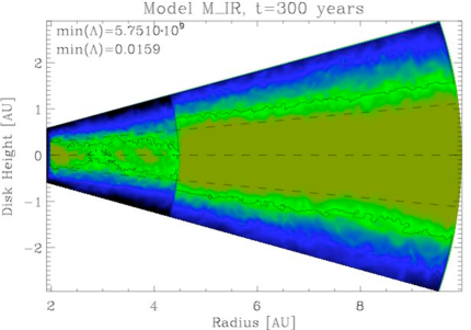
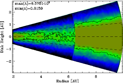
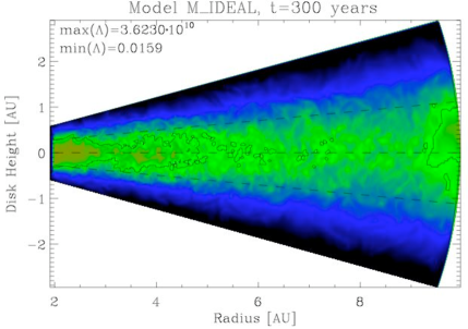
Figure 3: Elsässer number $\Lambda=v_{{\rm A}z}^{2}/\eta\Omega$ for models $\rm M_{IR}$ (top), $\rm M_{IR6}$ (middle) and $\rm M_{IR}$ (bottom). The Elsässer number is plotted in logarithmic color scale for edge-on view of the disk. Yellow-green color marks weak $B_{\Theta}$ magnetic fields which are stable to MRI. Blue is marking the regions with the vertical magnetic field sufficiently strong to launch the MRI. The transition to stability at $v_{{\rm A}z}^{2}/\eta\Omega=1$ is indicated with a black line. Slices of turbulent magnetic fields are taken for $t=300$ years (orbits at 1 AU) for each model.

The effective resolution of $10.47$ is holding during the linear stage of AMRI. The azimuthal magnetic field is breaking into filaments of opposite signs with $\lambda_{\Theta}<\lambda_{r}<<\lambda_{\phi}$ in MRI-active zones. The inverse plasma beta grows to 100 at the midplane and the decreases below unity in the upper disk layers. The effect of expelling the magnetic field into the corona becomes visible after 30 local orbits (section 3.2, Fig. 6). Note, that in low-resolution tests with $\lambda_{\rm c}/\Delta{\phi}=2.62$ ($\rm M_{IDEAL}$ with resolution of $r:\Theta:\phi=[64:16:8]$, excluded from Table 1), there is no MRI exited and the azimuthal magnetic field remains in its initial shape for few hundred years.

Fig. 2 demonstrates how the inverse plasma beta, $1/\beta=P_{\rm mag}/P_{\rm gas}$, changes due to MRI from $P_{\rm mag}/P_{\rm gas}=1/25$ (red dotted line) to the convex shape (black lines). The solid line stands for inverse plasma beta averaged within the active zone ($2.5\to 4.5$ AU). The dashed line stands for the $1/\beta$ averaged over the patch of the dead zone ($5\to 7$AU). In the midplane we find the minimum of magnetic pressure, with $P_{\rm mag}/P_{\rm gas}=0.01$. The plasma beta is reaching 1 at 2.8 H both in model $\rm M_{IR}$ and in the low-resolution run $\rm M_{IR/2}$ (Fig. 2, left). The resulting vertical profile of the magnetic pressure is very similar to those shown in Fromang & Nelson (2006). It is remarkable, that the dead zone builds up the same vertical distribution of magnetic pressure as the active zone, predominantly due to the smooth azimuthal magnetic field component. Radial dependence of the inverse plasma beta (Fig. 2, right) in the normal resolution run $\rm M_{IR}$ shows that upper layers possess the constant $P_{\rm mag}/P_{\rm gas}$, whereas the midplane layers, i.e. from midplane to 2H, are oscillating and slightly decrease towards the inner radius within the active zone. The dotted line in Fig. 2 (top right, model $\rm M_{IR}$) shows that the magnetic pressure falls to zero at $r=5.5\rm AU$ at the midplane. The reason is a diffusion of the mean azimuthal magnetic field from the active zone into the dead zone. This diffused field has the opposite sign to the primordial field. Its time propagation into the dead zone is shown in Fig. 4 (section 3.2). The low-resolution model $\rm M_{IR/2}$ shows that the expelling of the azimuthal field into the corona is not reaching the same extend as in the normal resolution model for radii $r>6$AU.

This vertical re-distribution of the azimuthal magnetic field affects the effective resolution. In the left panels of Fig. 2, we adopt solid lines for active and dashed lines for dead zone values. Green vertical bars in Fig. 2 mark the midplane region with $\lambda_{\rm c}/\Delta\phi<8$ (Eq. 11). The blue vertical bars show the disk height where Elsässer number $\Lambda=v_{{\rm A}z}^{2}/\eta\Omega$ drops below unity. The criterion for MRI instability $\Lambda>1$ has been introduced in Sano & Stone (2001) for the case of non-ideal MHD with Ohmic dissipation. After 300 years, the $B_{\phi}$ vertical profile is changed so much that the midplane layers are resolved only with $\lambda_{\rm c}/\Delta\phi\geq 5$, for example in the active zone (2.5 AU to 4.5 AU) in normal resolution model (green bars, Fig. 2). On the other side, model $\rm M_{IR/2}$ becomes well-resolved in the layers $|z/H|>2$. Effective resolution of $\lambda_{c}/\Delta\phi>16$ is reached in the active layers above the dead zone, where vertical MRI is launched outside of the $\Lambda=1$ line. Interesting to note, that the Elsässer number $\Lambda=v_{{\rm A}z}^{2}/\eta\Omega$ drops below unity roughly at the same height, when we compare normal and low resolution models (Fig. 2, top left and bottom left). When looking for numerical values of $\lambda_{\rm c}/\Delta\phi$ get at the location of blue bars in the active zone, we find $\lambda_{\rm c}/\Delta\phi=6$ for $\rm M_{IR}$ and 4 for $\rm M_{IR/2}$. These numbers are only approximate values, because it is difficult to calculate them accurately at the height at which $\Lambda=1$. All in all, there are surprisingly small differences between $\rm M_{IR}$ and $\rm M_{IR/2}$ models. The instability occurs in both cases and leads to similar physics, though the speed of the total field amplification is slower for $\rm M_{IR/2}$ (Table 1).

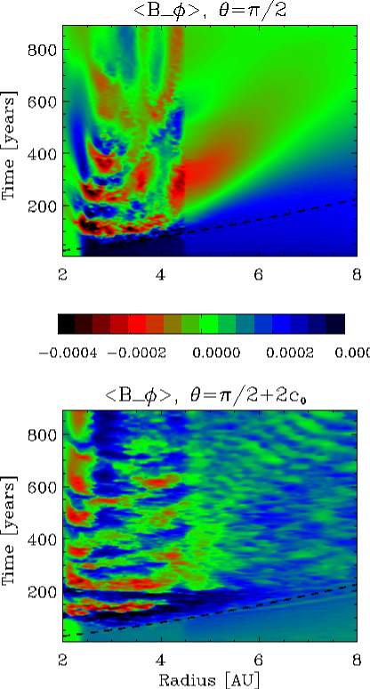
Figure 4: Temporal evolution of azimuthal magnetic field as a function of radius for $\rm M_{IR}$ model. Azimuthally averaged $B_{\phi}$ field is demonstrated for horizontal slices at $\Theta=\pi/2+n\cdot{}c_{0}$ or at $z=n\cdot{}H$, where $n=0,2$. In model $\rm M_{IR}$, the MRI-active zone reaches from $2.5$ to $4.5$ AU and layer $z=0$ is MRI-‘dead’ between $4.5$AU and $10$AU. The period of the $B_{\phi}$ sign reversals is about 150 years (30 local orbits). The black dashed line represents the time of 10 local orbits for each radius.

Fig. 3 demonstrates the Elsässer number and $\Lambda=1$ criterion in the $(r,\Theta)$ plane of azimuthally averaged disk. The solid black line of $\Lambda=1$ marks the locations where the regeneration of vertical magnetic field cannot be efficient enough. Models $\rm M_{IR}$ and $\rm M_{IR6}$ have their most active MRI layers at $2.5$H above the ’dead’ midplane. Comparison of the contour plots of the Elsässer number for $\rm M_{IR}$, $\rm M_{IR6}$ and $\rm M_{IDEAL}$ shows, that MRI-active zones have very similar appearance. At the midplane of the active zone, there are yellow-orange areas of low Elsasser number at $r\sim 4$AU ($\rm M_{IR}$, $\rm M_{IR6}$), $r\sim 4$AU ($\rm M_{IDEAL}$), and $r\sim 5.3$AU ($\rm M_{IR6}$), which are corresponding to the enhanced gas pressure. In section 3.4 we describe the formation of the density rings at these locations in more details. Condition $V_{\phi}/\eta\Omega>10$ is fulfilled in the whole disk in every model (Turner & Sano, 2008) and the magnetic fields may be pumped into the dead zone from the active layers.

3.2 Oscillating Magnetic Fields and Saturation

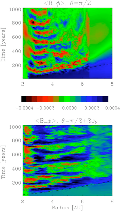
Figure 5: Temporal evolution of azimuthal magnetic field as a function of radius for $\rm M_{IR6}$ model. Azimuthally averaged $B_{\phi}$ field is demonstrated for horizontal slices at $\Theta=\pi/2+n\cdot{}c_{0}$ or at $z=n\cdot{}H$, where $n=0,2$. In model $\rm M_{IR6}$, the MRI-active zone reaches from $2.5$ to $6.5$ AU. The period of the $B_{\phi}$ sign reversals is about 150 years (30 local orbits), same as in Fig. 4. Model $\rm M_{IR6}$ demonstrates that sign reversal happens not only in time, but along the radius as well. The black dashed line represents the time of 10 local orbits for each radius.

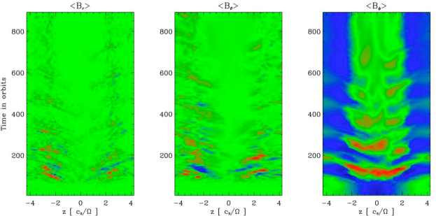
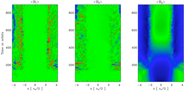
Figure 6: Horizontally averaged magnetic fields components $\langle{B_{r}\rangle}$, $\langle{B_{\Theta}\rangle}$ and $\langle{B_{\phi}\rangle}$ as function of disk height and time. Blue and red colors are tracing the positive and negative fields, green is always zero. $\langle{B_{\phi}\rangle}$ sign-reversals ‘swim’ from midplane to the disk corona (’butterfly diagram’). Above: model $\rm M_{\rm IR}$, averaging of the magnetic fields has been done within the MRI-active zone (between 2AU and 4AU). Below: model $\rm M_{\rm IR}$, averaging of the magnetic fields has been done within the dead zone (between 6AU and 8AU).

After most of the initial azimuthal magnetic flux has been shifted to the upper disk layers, the two scale heights to the adjacent midplane develop the oscillating axisymmetric magnetic field. For model $\rm M_{IR}$, the oscillations last for over 400 years and then decay. In the MRI-active zone, i.e. between 2.5 and 4.5 AU, the $B_{\phi}$ sign-switching occurs within about every 120 to 150 years. In Fig. 4 we demonstrate the time evolution of the azimuthally averaged $B_{\phi}$ as a function of the radial distance for the $\rm M_{IR}$ model. The fluctuating part of the azimuthal magnetic field is roughly ten times stronger than the mean part, $B_{\phi}^{{}^{\prime}}\sim 10\langle{B_{\phi}\rangle}$.

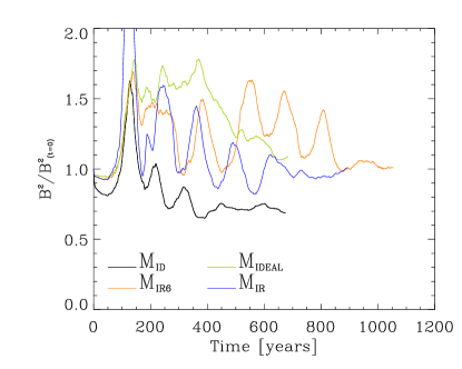
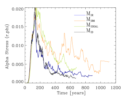
Figure 7: Top: Total magnetic energy evolution; Bottom: Total alpha stress evolution for models $\rm M_{IR}$, $\rm M_{ID}$, $\rm M_{IR6}$ and $\rm M_{IDEAL}$. The oscillations are correlated with the ‘butterfly diagram’.

This property appears to be typical for MRI, as the observations of the magnetic fields in the galactic disks show (see Beck (2000) for review). When the active zone is stretched up to $6.5$ AU, it is not affecting the time period of the $B_{\phi}$ sign reversals. Model $\rm M_{IR6}$ demonstrates that sign reversals occur not only in time, but also along the radius, as shown in Fig. 5. The first positive $B_{\phi}$-stripe is starting at 60 years at 3 AU and progresses to 6 AU in 160 years (Fig. 5). The stripes of $B_{\phi}$ in $(r,t)$-plane are stretched along the line of local orbit, which is plotted with black dashed line for $t_{\rm local}=10$ in Fig. 5. At later times, the mixing and interaction of the waves is breaking radial $B_{\phi}$ reversals into less regular oscillations both in Fig. 4 and in Fig. 5. The field diffusion in the dead zone outside of $r_{\rm th}=4.5$ AU (model $\rm M_{IR}$) and outside of $r_{\rm th}=6.5$ AU (model $\rm M_{IR6}$) does not follow the line of local orbit, $\propto r^{3/2}$, but propagates with diffusion time $\propto r^{2}$. For the $\rm M_{IR}$ run, the region with $r>4.5\ {\rm AU}$ develops the negative azimuthal magnetic fields due to diffusion of the magnetic field. After 600 years there is a weaker wave of positive $B_{\phi}$, which has a shorter time period.

Oscillations in the sign of $B_{\phi}$ at the $z\geq 2$H appear less clearly, compared to the azimuthal magnetic field at the midplane (Fig. 4, Fig. 5). A comparison with $\rm M_{ID}$ shows why. The reason is the interaction of MRI waves in the upper layers between active and dead zones. For the case of a very thick dead zone ($\rm M_{ID}$), the sign reversals in $B_{\phi}$ at $z=2H$ show most pronounced intervals. This is due to the fact, that MRI can be best exited between 1H and 2H layers of the active zone. In the model $\rm M_{IR}$, the layers above and below the dead zone are turbulent and interacting with MRI modes at same height in the active zone, what leads to a more irregular picture in oscillations of $B_{\phi}(r,t)$ at $z\geq 2$H. The color-coded presentation of $B_{\phi}$ as a function of $(z,t)$ reveals a butterfly diagram, if the azimuthal magnetic field is averaged within the disk region between 2 and 4 AU (Fig. 6, top). The low plasma $\beta$ does not prevent the upper disk layers from being very turbulent, as one can see from left and middle panels for $B_{r}$ and $B_{\Theta}$. Comparing the contours of dominating $B_{\phi}(z,t)$ and other two turbulent field components $B_{r}(z,t)$ and $B_{\Theta}(z,t)$ demonstrates again that the MRI turbulence and vertical redistribution of azimuthal magnetic field are connected. The period of $B_{\phi}$ oscillations is about 150 years, corresponding well to the radial changes of $B_{\phi}$ sign shown in Fig. 4 and Fig. 5. When averaging over the whole radial extent of the disk, or at least within the dead zone, then the butterfly picture disappears (Fig. 6, bottom).

Table 2: $\alpha$-stresses inside (A) and outside (D) of the ionization threshold radius for four layers above the midplane

Models/	$\rm M_{IR}$		$\rm M_{ID}$		$\rm M_{IR6}$		$\rm M_{IDEAL}$	$*$
/$\alpha$ stress	(A)	(D)	(A)	(D)	(A)	(D)	(A)
$\alpha_{\pm{}1H}\cdot{10^{-4}}$	2.69	0.83	2.86	1.13	4.18	1.22	5.30
$\alpha_{\pm{}2H}\cdot{10^{-4}}$	4.64	0.69	3.76	0.65	7.64	2.01	7.13
$\alpha_{\pm{}3H}\cdot{10^{-4}}$	10.53	7.63	7.82	0.49	15.98	11.48	12.80
$\alpha_{\pm{}4H}\cdot{10^{-4}}$	1.14	1.00	1.75	0.59	1.41	1.62	1.93

Volume-averaging of the magnetic energy shows, that its total value is oscillating in time, with a period correlated to the sign-switch in azimuthal magnetic field within $\pm 2H$ relative to the midplane. Fig. 7 shows the magnetic energy for each model in Table 1 and the corresponding total alpha stresses. The oscillations of energies in time can be clearly correlated with the butterfly diagram. Oscillations are weakly visible in the total alpha stress (Fig. 7, right). The magnetic energy curves reach a constant value in model $\rm M_{IR}$, which has the smallest active zone (from $2.5$ to $4.5$ AU). Model $\rm M_{ID}$ looses the total magnetic energy continously during 400 years due to higher magnetic dissipation. Model $\rm M_{ID}$ reaches a steady-state when stresses and magnetic energy remain unchanged from 400 to over 600 years. The longer is the MRI-active domain, the longer it takes for the simulation to reach the steady-state. Models $\rm M_{IR6}$ and $\rm M_{IDEAL}$ hold oscillatory (non-stationary) magnetic fields for 900 years.

The closed boundary conditions enforce the conservation of the total flux in the domain. Fluxes of vertical magnetic field remain zero through the whole simulation. The effect of the boundary choice on the butterfly diagram remains to be investigated in future work. The local box simulations, made for open vertical boundaries, show the butterfly picture as well (Turner & Sano, 2008).

3.3 Maxwell and Reynolds Stresses

Radial inhomogeneity in turbulent viscosity has been suggested as the mechanism to produce the pressure maximum, which is efficient in dust trapping, and therefor important in the planet formation theory. In our models, the turbulent viscosity is driven by MRI and the inhomogeneity in turbulent stresses appears naturally as the result of simulations, when we include the sharp gas ionization threshold. Indeed, we find a density bump forming behind the ionization threshold in our simulations (section 3.5), and a corresponding jump in turbulent $\alpha$ stress.

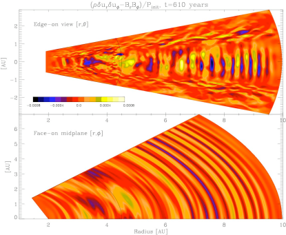
Figure 8: Snap-shots of turbulent $\alpha$ stress in $(r,\Theta)$ (top) and $(r,\phi)$ (bottom) slices for models $\rm M_{IR}$ for data output at $t=610$ years. Black line indicates the ionization threshold.

The time evolution of the Maxwell stress $T_{\rm M}(r,t)$ (Eq. 9) is demonstrated in Fig. 9. There is a weak Maxwell stress of about $10^{-5}$ in the dead zone, which can periodically become negative. One can see the sharp border in $T_{\rm M}(r,t)$ between the active and the dead zones in slices for $z=0$, $z=1H$ and $z=2H$. The traces of sign reversals in the azimuthal magnetic field are also visible in the Maxwell stress. Fig. 9 shows that exactly at 150 years the Maxwell stress reaches its maximum of $10^{-1}$, when calculated in units of initial pressure $\langle{P(r)\rangle}$ (Eq. 9). Later on, the saturation of MRI sets in and the total stress is between $10^{-3}$ and $10^{-2}$ (see Table 1). The dark-orange filaments of very weak Maxwell stress in the active zone, $\pm 10^{-7}$, correspond to the location where the reversals of axisymmetric azimuthal field happen. The weak Maxwell stress is located at $r=3.5$ AU for many years, what appears as a systematic stripe when looking at $z=0$ and $z=1H$ horizontal slices of $T_{\rm M}(r,t)$ in Fig. 9. This is a location where the density ring is created (more in section 3.4) and also most of $B_{\phi}$ reversals take place during the time period from 200 to 700 years. Negative values of Maxwell stress appear at 3H above the midplane. This is the region of low plasma beta, and the turbulence at this height is no more MRI-driven.

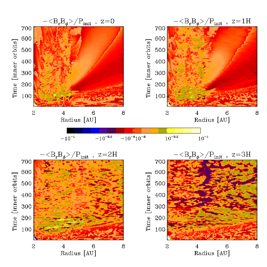
Figure 9: Model $\rm M_{IR}$: temporal and radial evolution of Maxwell stress. Horizontal slices of $T_{\rm M}(r,t)$ are taken at $\Theta=\pi/2+n\cdot{}c_{0}$ or $z=n\cdot{}H$, where $n=0,1,2,3$. The color scale shows the azimuthally averaged Maxwell stress in local gas pressure units. Dark-orange filaments ($\pm 10^{-7}$) in the active zone correspond to the location where the reversals of axisymmetric azimuthal field happen. Weak Maxwell stress of $\pm 10^{-5}$ also occurs in the dead zone.

In the dead zone, the value $\alpha_{\rm total}\sim{10^{-3}}$ is due to Reynolds stress contribution. In order to provide the understanding of how the turbulence there looks like, we present a snap-shot of turbulent $\alpha$ stress for the $\rm M_{IR}$ model (Fig. 8). The dead zone is filled with vertical pillars of the $\alpha$ stress of opposite sign. In the $(r,\phi)$ plane, those pillars look like tightly-wrapped spirals. The spiral waves are launched from the dead-zone edge ($r_{\rm th}=4.5$ AU), where the non-axisymmetric fluctuations in all velocity components are MRI-generated. The weak spiral structures can be found in the gas density as well.

We have calculated the turbulent stresses as the function of radius. The vertical averaging has been done separately for four midplane-symmetric layers: $|\Theta-\pi/2|<c_{0}$, $c_{0}<|\Theta-\pi/2|<2c_{0}$, $2c_{0}<|\Theta-\pi/2|<3c_{0}$ and $3c_{0}<|\Theta-\pi/2|<4c_{0}$, where $c_{0}=H/R=0.07$. The resulting $\alpha$ stresses for these layers are given in Table 2 as $\pm{}1H,\ 2H,\ 3H,\ 4H$ correspondingly and plotted in Fig. 10 and Fig. 11 with solid, dotted, dashed and dot-dashed black lines. In Table2, the mark $*$ indicates that the steady-state has not yet been reached. Solid blue lines in Fig. 10 and Fig. 11 represent the $\alpha(r)$ integrated over the whole disk thickness. The strongest total stress alpha of all models is obtained in model $\rm M_{IDEAL}$, which remains of the same order of magnitude with radius.

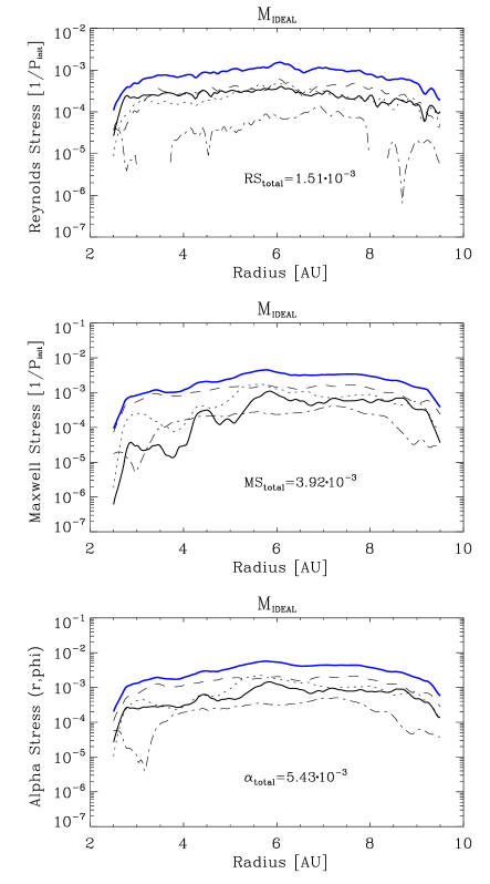
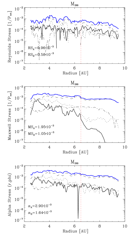
Figure 10: Reynolds, Maxwell and total $\alpha$ stresses for models $\rm M_{IDEAL}$ (left) and $\rm M_{IR6}$ (right). Vertical averaging of stresses is made separately for four midplane-symmetric layers, $\pm{}\ 1H({\rm solid\ line}),\ 2H({\rm dotted\ line}),\ 3H({\rm dashed\ line}),\ 4H({\rm dot-dashed\ line})$. Solid blue line shows the classical total stress. All stresses are normalized to the pressure at $t=0$. Time average is made between 850 and 1050 years for $\rm M_{IR6}$, and between 610 and 681 years for $\rm M_{IDEAL}$.

The turbulent stresses have $\propto r^{-2}$ slope during the ’butterfly’ evolution stage in models $\rm M_{IR6}$ and $\rm M_{IR}$. For the $\rm M_{IR}$ model, the time averaging of the stresses between 250 and 600 years results in a $\alpha\propto r^{-2}$. Afterwards, the turbulence in $\rm M_{IR}$ reaches a ’butterfly’-free state ($t>600$ years). When the temporal averaging is made between 400 and 800 years, instead of from 250 to 600 years, we obtain $\alpha_{\rm A}$ which is constant with radius (Fig. 11). In the $\rm M_{IR}$ model, the Maxwell stress is the main contribution to $\alpha_{\rm total}$ only for layers $\ 3H,\ 4H$ outside the threshold $r_{\rm th}=4.5\rm AU$ (Fig. 11).

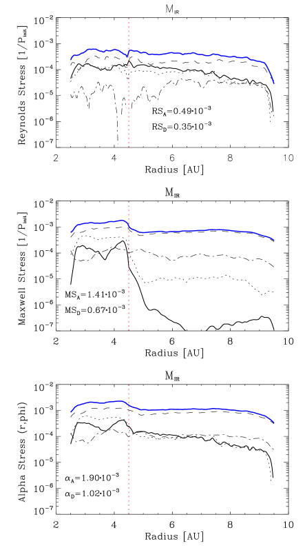
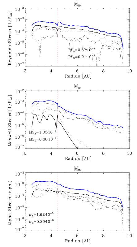
Figure 11: Reynolds, Maxwell and total $\alpha$ stresses for models $\rm M_{IR}$ (left) and $\rm M_{ID}$ (right). Vertical averaging of stresses is made separately for four midplane-symmetric layers, $\pm{}\ 1H({\rm solid\ line}),\ 2H({\rm dotted\ line}),\ 3H({\rm dashed\ line}),\ 4H({\rm dot-dashed\ line})$. Solid blue line shows the classical total stress. All stresses are normalized to the pressure at $t=0$. Time averages has been done starting from time of 400 years until the last data output.

The gas density perturbations look like spiral waves, and the Maxwell stress is strongly reduced outside of the ionization threshold. Model $\rm M_{ID}$ shows a steeper fall in Reynolds stress and in total $\alpha$ in the dead zone, compared to the $M_{\rm IR}$ model. The active layers above and below the dead zone are very thin and only marginally unstable to MRI. Model $\rm M_{ID}$ has $1H,\ 2H$ and partly $3H$ layers which are deactivated in the dead zone. The pumping of the waves happens mostly from the MRI-active zone, and not from both active zone and adjacent layers as in $\rm M_{IR}$. Comparing models $\rm M_{IR}$ and $\rm M_{ID}$, we conclude that the pumping of the hydro-dynamical waves into the dead zone is coming both from ’sandwich’ active layers and from the active zone within $r_{\rm th}$.

The summary of turbulent $\alpha$ stress values for each layer above the midplane is presented in Table 2. The radial averaging has been done separately for active (A) and dead (D) zones. The turbulent $\alpha_{\rm(A)}$ stress is increasing from midplane to $2c_{0}<|\Theta-\pi/2|<3c_{0}$, and drops in the fourth layer. The most prominent decrease in $\alpha$ stress from active to dead zone happens within adjacent to the midplane $|\Theta-\pi/2|<2c_{0}$ layers for models $\rm M_{IR}$ and $\rm M_{IR6}$. In the case of very thick dead zone ($\rm M_{ID}$), the decrease in turbulent stress at the dead zone edge is significant in all three layers, $|\Theta-\pi/2|<3c_{0}$.

3.4 Development of Pressure Maxima and Trapping of Solids

Due to active secretion through MRI-active zone, the pressure bump at the inner edge of the dead zone is formed within a hundred of inner orbits.

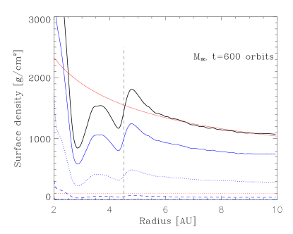
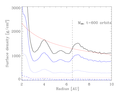
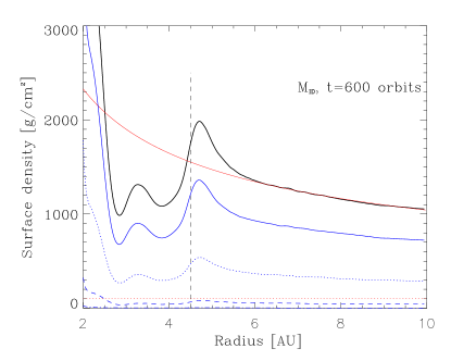
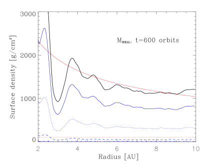
Figure 12: Surface density after 600 years of evolutions. Red solid line stands for the initial surface density profile, black solid line represents the final surface density. Red dotted line indicates the cosmic ray adsorbtion depth $100\rm g/cm^{2}$. Blue lines show the contributions of every scale height in the surface density. Vertical dashed line shows the inner edge of the dead zone.

The change in the radial density gradient appears in the disk layers starting from the midplane and up to 3H. The piling up of the density behind the $r_{\rm th}$ is accompanied by a broad gap before the threshold. In addition, we find the rings of enhanced density within the MRI-active zone. The pressure bump at the inner edge of the dead zone and the rings of enhanced density within the MRI-active zone are formed due to different processes, which we discuss in section 4. Fig. 12 (top) shows the changes of surface density for models $\rm M_{IR}$ and $\rm M_{IR6}$. In our simulations, the number of density rings depends on the extension of the active zone. In the model without a dead zone, there are three rings of enhanced density appearing within the domain before the quasi steady-state is reached (Fig. 12, bottom right). The thicker dead zone (model $M_{\rm ID}$) seems to be more efficient in piling up the higher bump: the maximum of the surface density peak is larger, when compared to the snap-shots of surface density in $\rm M_{IR}$ at the same time.

First, we consider the accumulation of the density at the inner edge of the dead zone. The pressure bump is fixed in time at the location behind the ionization threshold $r_{\rm th}$, as in Fig. 13 (left). There are three stages in the evolution of the pressure maximum at the inner edge of the dead zone (Fig. 13, middle), for example when considering model $\rm M_{IR}$. One can recognize the period of very fast mass excavation for the time from $t=0$ to $150$ years. During $t=150\to 600$ years the peak of surface density is still growing at a roughly ten times slower speed. After $t=600$ years there is no further increase of surface density, what corresponds to the steady-state in the presence of saturated MRI-turbulence. The most straight-forward explanation for three stages in density excavation gives a time-dependent evolution of the Maxwell stress, since it governs the accretion in the MRI-active zone and in the active layers. The quasi-steady state is reached for models $\rm M_{IR}$ and $\rm M_{ID}$ after 600 years, and the maximum of the pressure bump at the ionization threshold and the minimum of the surface density in the gap remain unchanged. The density rings in the active zone appear to be long-living but less stable features. We observe the merging of two rings of enhanced density after 640 years in model $\rm M_{IR6}$ (Fig. 13, bottom).

The radial pressure gradient is negative in the smooth unperturbed disk, what leads to sub-Keplerian gas rotation. Dust grains undergo an orbital decay (Adachi et al., 1976), because they experience the ’head’ wind. For example, the meter-size particle will migrate from 1 AU into the Sun within few hundred years (MMSN model). When local positive exponent of the disk midplane pressure appears, the dust grains may experience ’tail’ wind and the hydrodynamical drag will lead to their outward migration (Nakagawa et al., 1986). The criterion for outward migration of the dust grain due to the gas drag is

$$p>-q/2+3/2,$$ (12)

where $p=d\log{\Sigma_{\rm gas}}/d\log{r}$ and $q=2d\log{c_{\rm s}}/d\log{r}$. Note that the factor $3/2$ is the normalized shear. The planetary embryos can be stopped in such pressure traps as well (Zhang et al., 2008). Criterion for outward migration of the protoplanetary cores has been given in Ida & Lin (2008) and is based on the migration rate of planets (Tanaka et al., 2002). When curvature effects on the Lindblad resonances have been included, the condition for outward migration for embryos is

$$p>-0.80q+2.52.$$ (13)

The right panels in Fig. 13 show where criteria for outward migration are fulfilled in our models. Black lines stand for criterion given in Eq. 12 and the red dashed line is for Eq. 13. The outward migration of planetesimals is possible within the pressure bump at the inner edge of the dead zone (Fig. 13). Conditions for embryos are more difficult to satisfy. Not all density rings within the active zone provide sufficiently strong positive pressure gradients, so that planetary embryos cannot be stopped there. The exception is model $\rm M_{IR}$. There we obtain two pressure traps at $r=3$ AU and at $r=4.5$AU, where large bodies can be retained.

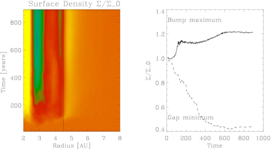
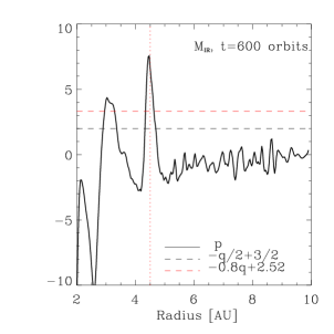
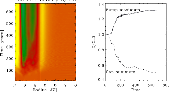
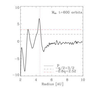
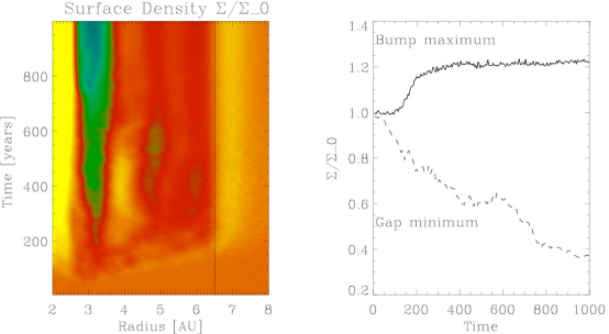
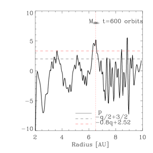
Figure 13: Relative surface density $\Sigma/\Sigma_{0}$, for models $M_{\rm IR}$ (above), $M_{\rm ID}$ (middle) and $M_{\rm IR6}$ (below). Left: Colors show the evolution of density bumps (yellow) and gaps (green). Middle: time development of $\max(\Sigma/\Sigma_{0})$ of the bump at $r=[3:6]$AU and $\min(\Sigma/\Sigma_{0})$ of the gap in $r=[2.5:5]$AU. Right: Criteria for outward migration (Eqs. 12, 13). Rings of enhanced density are formed in the active zone and the outmost density ring is located at the ionization threshold, marked as a vertical line in both left and right panels.

3.5 Super-Keplerian Rotation and Similarity to Zonal Flows

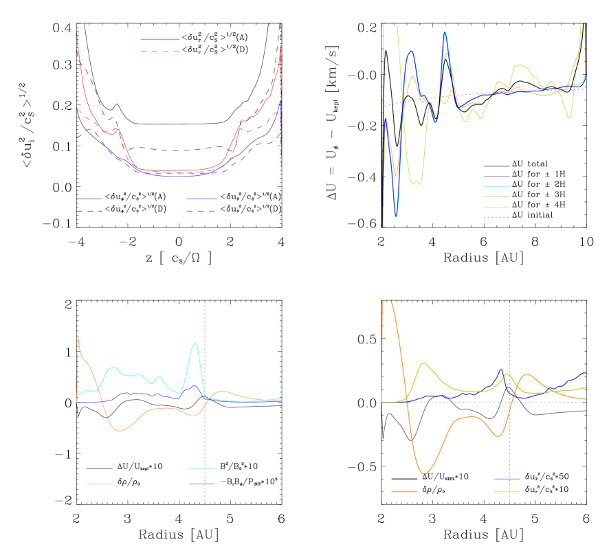
Figure 14: Radial and vertical turbulent properties in model $\rm M_{IR}$. Top left: root-mean-square turbulent velocities are averaged separately for active (A) and for dead (D) zones. Top right: Outward migration velocity. Panels on bottom right and bottom left show time-averaged density, Maxwell stress, magnetic energy and r.m.s. velocities at the midplane. Time average is from 600 to 800 years (steady-state stage in model $\rm M_{IR}$).

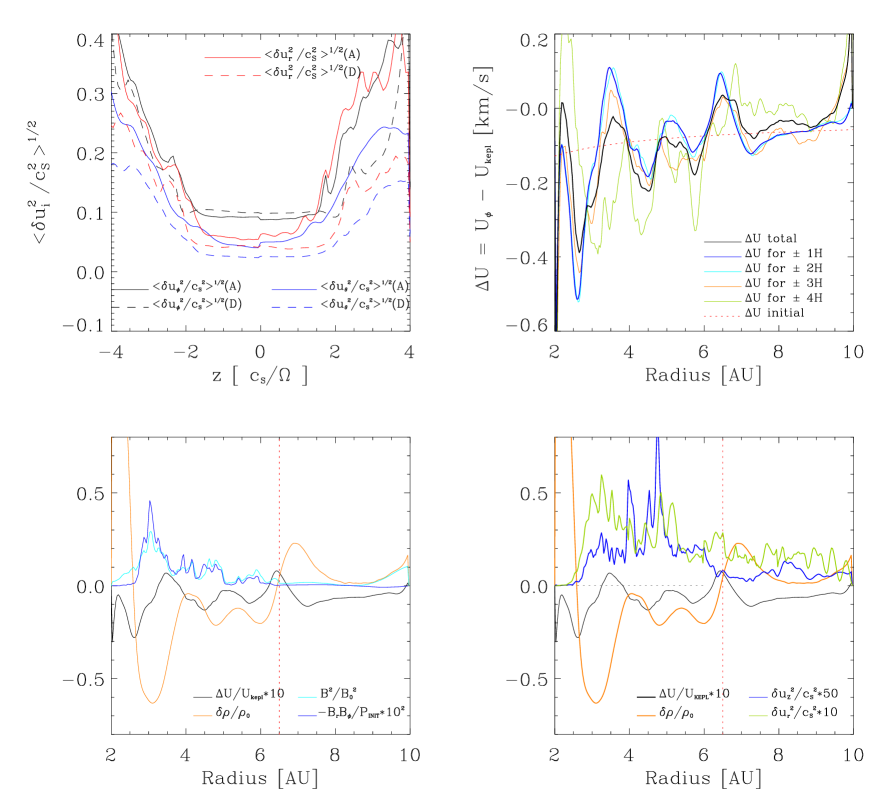
Figure 15: Radial and vertical turbulent properties in model $\rm M_{IR6}$. Top left: root-mean-square turbulent velocities are averaged separately for active (A) and for dead (D) zones. Top right: Outward migration velocity. Panels on bottom right and bottom left show time-averaged density, Maxwell stress, magnetic energy and r.m.s. velocities at the midplane. Time average is from 900 to 1100 years.

When a quasi-steady state is reached, all time derivatives can be neglected and the Navier-Stokes equation for radial velocity gives:

$$-\frac{u_{\phi}^{2}}{r}=\frac{\partial\Psi}{\partial r}-\frac{1}{\rho}\frac{\partial c_{\rm s}^{2}\rho}{\partial r}+F_{\rm lorentz}.$$ (14)

In our locally-isothermal simulations, the temperature is constant on cylinders. The steady-state solution is then given as

$$-\frac{(u_{\phi}^{2}-u_{\rm kep}^{2})}{u_{\rm kep}^{2}}=-\frac{rc_{a}^{2}}{\sin{\Theta}}\left(-\frac{1}{r}+\frac{\ln(\rho)}{\partial r}\right)+\frac{r}{u_{\rm kep}^{2}}F_{\rm lorentz}.$$ (15)

It follows from the last equations, the gas may reach purely Keplerian rotation when the density profile is locally changed to $\rho\propto r$ and the Lorentz forces are negligibly weak.

The vertical profiles of turbulent velocity dispersion and the mean radial drift velocity $\Delta U=u_{\phi}-u_{\rm kepl}$ are plotted in Fig. 14 ($\rm M_{IR}$) and Fig. 15 ($\rm M_{IR6}$). The root-mean-square turbulent velocities can be described with the same shape of the vertical profile both in the active and in the dead zone. The turbulent velocity dispersion reaches 0.4 in the corona. This agrees with the result of Fromang & Nelson (2006). The top left panels in Figs. 14 and Fig. 15 show the root-mean-square turbulent velocities averaged separately for active (A) and for dead (D) zones. It is interesting to note, that the levels of $\sqrt{<u_{\Theta}^{2}/c_{s}^{2}>}$, $\sqrt{<u_{r}^{2}/c_{s}^{2}>}$ at the midplane are not very different for the two zones. Midplane values vary from 0.03 for $\sqrt{<u_{\Theta}^{2}/c_{s}^{2}>}$ to 0.16 for $\sqrt{<u_{\phi}^{2}/c_{s}^{2}>}$. As expected, the perturbations of rotational profile are higher in the active zone. The radial dependence of $\sqrt{<u_{\Theta}^{2}/c_{s}^{2}>}$, $\sqrt{<u_{r}^{2}/c_{s}^{2}>}$ shows that the turbulent dispersion is significantly reduced within the pressure bump at the inner edge of the dead zone (Fig. 14 and Fig. 15, bottom right).

The time-average of $\Delta U$ shows that the super-Keplerian rotation at the density rings is a long-lasting effect. Relatively large dust particles (i.e. for Stokes number $\rm St=1$) will migrate outwards with the velocity $v_{r}=\Delta U$ (Klahr & Lin, 2001). The areas of outward migration are up to $0.5AU$ broad and outward velocities reach 0.15 km/s (Fig. 14 and Fig. 15, top right).

There are certain similarities between the density bump and rings we found and the zonal flows described in Johansen et al. (2009). The enhancement in density has been reaching 10 pressure scale heights both in large local-box simulations and in the global model of Lyra et al. (2008). We estimate the rings to be roughly 1.5 AU broad, what gives maximum 6 pressure scale heights. We show the radial correlations of the following parameters: $\Delta U=u_{\phi}-U_{\rm Kepl}$ for various heights in the disk, $\delta\rho/\rho_{0}=(\rho-\rho_{0})/\rho_{0}$, magnetic pressure $B^{2}/B_{0}^{2}$, and Maxwell stress $B_{r}B_{\phi}/P_{\rm init}$ (Fig. 14, Fig. 15, bottom left). The gas around the rings of enhanced density within the active zone in $\rm M_{IR6}$ and $\rm M_{IR}$ models shows similar turbulent properties to the zonal flows and corresponding density maximum as in Johansen et al. (2009): The magnetic pressure and Maxwell stress are strongest where the density minima are excavated, the maximal $\Delta U$ is half-phase shifted. The maximal deviations from Kepler velocity have same amplitude as in zonal flows in Johansen et al. (2009), but the relative amplitude of density $\delta\rho/\rho_{0}=(\rho-\rho_{0})/\rho_{0}$ is ten times larger in our models. The maxima of magnetic pressure $B^{2}/B_{0}^{2}$ and Maxwell stress $B_{r}B_{\phi}/P_{\rm init}$ are located between the rings and are about ten times stronger compared to the values in Johansen et al. (2009).

In addition, the pressure bump at the ionization thresholds has significantly less turbulence; the $u_{\Theta}^{2}/c_{\rm s}^{2}$ has a value only about 0.05 and not 0.5 as outside of the density bump. In the case of $\rm M_{IR}$, the density ring in the active zone is a ’calm place’ as well. Model $\rm M_{IR6}$ keeps the butterfly pattern of the azimuthal fields much longer. This is the reason why the turbulent velocities decrease in the density rings weaker in the case of $\rm M_{IR6}$, compared to $\rm M_{IR}$.

4 Synthesis: Connection Between Pressure Maxima and ‘Butterfly’ Structures

4.1 Density Rings in the MRI-Active Region

In order to provide the comparison with previous global simulations (Fromang & Nelson, 2006), we have done the fully MRI-active disk model. The turbulent and magnetic properties of the fully MRI-active disk model $\rm M_{IDEAL}$ are very close to those presented in Fromang & Nelson (2006) for run S4. The toroidal magnetic field is expelled from the midplane into the upper disk layers within the linear stage of MRI turbulence. The peak value of the volume-integrated turbulent $\alpha$ stress is reaching 0.019 in our model $\rm M_{IDEAL}$ (Fig. 7) and 0.013 in the S4 model (Fromang & Nelson, 2006). At the end of the simulation, the turbulent $\alpha$ stress is $0.005$ in gas pressure units.

In our simulations, the MRI turbulence evolves through three stages: (a) linear growth, (b) oscillatory saturation regime and (c) non-oscillating steady state. The stage (b) is best to observe if the dead zone is included. The oscillations are regular and can be registered in total magnetic energy and in turbulent $\alpha$ stress time evolution. The dominating azimuthal magnetic field component in the MRI-active zone switches its sign with a period of about 150 years or 30 local orbits, and within the radial extent of 1.5 AU. The sign reversals of the azimuthal magnetic field with respect to the midplane, known as butterfly diagram, have also been observed in local shearing-box simulations of the stratified disk (Turner et al., 2007; Johansen et al., 2009). In case of the global simulation (model $\rm M_{IDEAL}$), averaging over the whole eight AU of the MRI-active domain brings a very irregular butterfly picture. Numerous reversals of the azimuthal magnetic field along the radial extent lead to seemingly irregular peaks in $\alpha(r)$ and in the magnetic energy.

We observe in our models, that the reversals in $B_{\phi}$ come along with the density rings. Thus, it is important to understand what causes radial and temporal reversals in the magnetic field, and what determines a period. We observe that the amplitude of the oscillations in magnetic energy is higher, if we increase the radial extent of the active zone (models $\rm M_{IR}$ and $\rm M_{IR6}$). In addition, it is important to know how long the ’butterfly’ structure can survive. The magnetic field is oscillating over the whole duration of the local-box simulations. In our global runs, the life-time of the oscillating stage (b) seems to depend on the extent of the MRI-active zone (Fig. 7). The thickness of the dead zone also influences the life-time of the oscillatory regime (b), as we found from a comparison of magnetic energy curves for models $\rm M_{IR}$ and $\rm M_{ID}$. The MRI waves in active layers above and below the dead zone are interacting with the turbulent magnetic field inside the threshold radius. If the layers above and below the dead zone are as thin as in our model $\rm M_{ID}$, the turbulent $\alpha$ stress in the active zone appears to be lower, the same applies to the total magnetic energy. The oscillations of the azimuthal magnetic field have ceased after 400 years, and after 600 years in the case of thinner dead zone (model $\rm M_{IR}$, Fig. 7). The turbulent $\alpha$ stress is roughly constant with radius during the non-oscillating steady stage (c).

The inner radial boundary with its resistive buffer (${2\rm AU}<r<2.5\rm AU$) and the inner edge of the dead zone $r_{\rm th}$ enclose the MRI-active zone in our models $\rm M_{IR}$, $\rm M_{ID}$ and $\rm M_{IR6}$. We observe a butterfly diagram in the MRI-active zone of our models, when plotting $\langle{B_{\phi}(z)\rangle}\propto t$. There are no oscillations of $\langle{B_{\phi}(z)\rangle}$ in or around of the dead zone. We obtain the clearest oscillations of $B_{\phi}$ at the midplane of active zone, $|\Theta-\pi/2|\leq{}c_{0}$. The $B_{\phi}$-sign reversal happens every 150 years and within $2.5\rm AU<r<4\rm AU$ (models $\rm M_{IR}$, $\rm M_{IR6}$) and $4\rm AU<r<5.5\rm AU$ ($\rm M_{IR6}$), i.e. within every $1.5$ AU. Those reversals are stretched along the line of the local orbit in $(r,t)$ space.

The rings of enhanced density appear already at $t=150$ years, roughly at the time when the linear AMRI breaks into a nonlinear regime and the ’butterfly’ is initiated. During the oscillatory stage (b) of the MRI evolution, there is a radial dependence in turbulent $\alpha$ stresses according to $\alpha(r)\propto r^{-2}$. At the inner radii, the $\alpha$ stress is high and it leads to the effect of fast local excavation of the density and accumulation of it at some outer radius. The radial reversals of the azimuthal magnetic field are aligned with the rings of enhanced density. The radial location of magnetic field reversals remains constant over hundreds of years. At the same location, we find the stripes of weakest Maxwell stress $\sim 10^{-7}$ (Fig. 11). As soon as the ring of density is created at a certain location, there is a corresponding change in the rotation and in the shear. On the one hand, over-density leads to the local $P_{\rm mag}/P_{\rm gas}$ relation which can be too low to excite AMRI. On the other hand, the change in the rotation reduces the shear and it leads to local stabilization of MRI within the density ring. The consequence is that the rings of enhanced density are less turbulent compared to the density minima between the rings. In contrast to the local-box studies (Johansen et al., 2009; Guan et al., 2009), there is more then one density ring forming in the case of a longish MRI-active zone. The merging between rings is possible. In the $\rm M_{IDEAL}$ model, we observe the appearance of three weak density rings.

4.2 Pressure Maximum at the Inner Edge of the Dead Zone

The formation of the pressure bump at the dead zone edge is not directly correlated with the ’butterfly’ magnetic structures within the active zone. The strength of the turbulent viscosity in the MRI-active zone determines the time scale to form such a pressure bump. The extent of the MRI-active zone has an effect on the value of the total turbulent $\alpha$ stress in the active zone. As it follows from Table 1, the turbulence in models $\rm M_{IDEAL}$ and $\rm M_{IR6}$ provide the largest stresses of $5.3\cdot{}10^{-3}$ and $2.9\cdot{}10^{-3}$, followed by $\rm M_{IR}$ with $1.9\cdot{}10^{-3}$ and $\rm M_{ID}$ with $1.6\cdot{}10^{-3}$. The radial extent of the active zone was reduced from 8AU to 4 AU and to 2AU. This sequence is consistent with the results of Guan et al. (2009); Bodo et al. (2008), where a similar decrease of total alpha stress is demonstrated when the size of the local box is reduced.

The jump in the turbulent viscosity is responsible for the formation of a pressure trap at the dead zone edge. This jump is strongest at the midplane. The intensity of MRI-driven turbulence grows strongly with the disk height. The locally calculated stresses are different for each pressure scale height layer: there is up to 1 order of magnitude difference when comparing the values for midplane and top $(|\Theta-\pi/2|>3c_{0})$ layers of the active zone. As expected, the midplane value of Maxwell stress decreases drastically in the dead zone, but the Reynolds stress does not ’feel’ the presence of the dead zone. We observe only a slight bump in the Reynolds stress at the location of the density maximum. Within the dead zone, there are spiral density waves propagating from the inner edge outwards. The vertical velocity dispersion is non-zero as well. We conclude that the resulting $\alpha$ of about $10^{-3}$ is due to the waves pumped vertically from the active layers and radially from the active zone through the threshold radius. For the disk evolution, it is important to have a significant residual $\alpha$ in the dead zone in order to reach the quasi-steady state without getting unstable (i.e., a gravitational instability of the density ring).

5 Conclusions

We have presented the results of the first global non-ideal 3D MHD simulations of stratified protoplanetary disks. The domain spans the transition from the MRI-active region near the star to the dead zone at greater distances. The main results are as follows.

• As suggested in Kretke et al. (2008), the height-averaged accretion stress shows a smooth radial transition across the dead zone edge. The stress peaks well off the midplane at $2c_{0}<|\Theta-\pi/2|<3c_{0}$. Consequently, averaging over the full disk thickness yields only a mild jump, despite the steepness of the midplane radial stress gradient.

• Weak accretion flows within the dead zone are driven mainly by Reynolds stresses. Spiral density waves propagating horizontally produce non-zero velocities and angular momentum transport near the midplane, apparently with little associated mixing. The dead zone midplane vertical velocity dispersion $|u_{\Theta}^{{}^{\prime}}|$ is $0.03$ times the sound speed, two to three times less than the radial and azimuthal components (Fig. 15). The waves are pumped both by the active region near the star and by the active layers above and below the dead zone. In model $\rm M_{ID}$ where the dead zone is very thick, the pumping from the surface layers is weak and the stress falls steeply with radius within the dead zone (Fig. 11).

• The excavation of gas from the active region during the linear growth and after the saturation of the MRI leads to the creation of a steady local radial gas pressure maximum near the dead zone edge, and to the formation of dense rings within the active region, resembling the zonal flows described in Johansen et al. (2009) (Fig. 12, Fig. 13). Super-Keplerian rotation is observed where the radial pressure gradient is positive. The corresponding outward radial drift speeds for bodies of unit Stokes number can exceed 10% of the sound speed. The pressure maxima are thus likely locations for the concentration of solid particles.

• The turbulent velocity dispersion, magnetic pressure and Maxwell stresses all are greatest in the density minima between the rings. The dense rings are ‘quiet’ locations where the turbulence is substantially weaker. Such an environment may be helpful for the growth of larger bodies.

• The rings within the active zone sometimes move about, leading to mergers. In contrast, the bump at the dead zone inner edge is stationary. Planetary embryos with masses in the type I migration regime can be retained at the dead zone inner edge as proposed by Ida & Lin (2008); Schlaufman et al. (2009).

6 Outlook

The causes of the magnetic field oscillations appearing in the butterfly diagram remain to be clarified. In particular, it is not known what processes drive the quasi-periodic reversals in the azimuthal magnetic fields shown in figure 4.

While we have used a fixed magnetic diffusivity distribution, the degree of ionization will in fact change as the disk evolves. Annuli of increasing surface density will absorb the ionizing stellar X-rays and interstellar cosmic rays further from the midplane, and will have higher recombination rates due to the greater densities. These effects will likely mean contrasts in the strength of the turbulence between the rings and inter-ring regions, even greater than those observed in our calculations. Stronger magnetic fields and higher mass flow rates in the inter-ring regions could lead in turn to growth in the surface density contrast over time, analogous to the viscous instability of the $\alpha$-model in the radiation-pressure dominated regime (Lightman & Eardley, 1974; Piran, 1978).

The resistivity can show another kind of time variation near the boundary of the thermally-ionized region. Changes in the temperature can alter the strength of the turbulence and thus the heating rate. In this way, radial heat transport can activate previously dead gas (Wünsch et al., 2005, 2006). Radial oscillations of the ionization front may be the consequence. Overall, due to the fixed magnetic diffusivity, it is probable that our models underestimate the evolution resulting from the ionization thresholds.

Owing to the effects of the radial boundary conditions, our global simulations have limitations for measuring quantities such as the accretion rate and the mean radial velocity. Fixing the rate of flow across the outer radial boundary is a promising avenue for further exploration in this direction.

Acknowledgments

N. Dzyurkevich acknowledges the support of the Deutsches Zentrum für Luft- und Raumfahrt (DLR). N. Dzyurkevich, M. Flock and H. Klahr were supported in part by the Deutsche Forschungsgemeinschaft (DFG) through Forschergruppe 759, “The Formation of Planets: The Critical First Growth Phase”. The participation of N. J. Turner was made possible by the NASA Solar Systems Origins program under grant 07-SSO07-0044, and by the Alexander von Humboldt Foundation through a Fellowship for Experienced Researchers. The parallel computations were performed on the PIA cluster of the Max Planck Institute for Astronomy Heidelberg, located at the computing center of the Max Planck Society in Garching.

References

- Adachi et al. (1976) Adachi, I., Hayashi, C., & Nakazawa, K. 1976, Progress of Theoretical Physics, 56, 1756
- Arlt & Rüdiger (2001) Arlt, R. & Rüdiger, G. 2001, A&A, 374, 1035
- Balbus & Hawley (1991) Balbus, S. A. & Hawley, J. F. 1991, ApJ, 376, 214
- Balbus & Hawley (1998) Balbus, S. A. & Hawley, J. F. 1998, Reviews of Modern Physics, 70, 1
- Beck (2000) Beck, R. 2000, in Royal Society of London Philosophical Transactions Series A, Vol. 358, Astronomy, physics and chemistry of , 777–796
- Benz (2000) Benz, W. 2000, Space Science Reviews, 92, 279
- Blum & Wurm (2000) Blum, J. & Wurm, G. 2000, Icarus, 143, 138
- Blum et al. (1998) Blum, J., Wurm, G., Poppe, T., & Heim, L.-O. 1998, Earth Moon and Planets, 80, 285
- Bodo et al. (2008) Bodo, G., Mignone, A., Cattaneo, F., Rossi, P., & Ferrari, A. 2008, A&A, 487, 1
- Brandenburg et al. (1995) Brandenburg, A., Nordlund, A., Stein, R. F., & Torkelsson, U. 1995, ApJ, 446, 741
- Brauer et al. (2008a) Brauer, F., Dullemond, C. P., & Henning, T. 2008a, A&A, 480, 859
- Brauer et al. (2007) Brauer, F., Dullemond, C. P., Johansen, A., et al. 2007, A&A, 469, 1169
- Brauer et al. (2008b) Brauer, F., Henning, T., & Dullemond, C. P. 2008b, A&A, 487, L1
- Dziourkevitch et al. (2004) Dziourkevitch, N., Elstner, D., & Rüdiger, G. 2004, A&A, 423, L29
- Fleming & Stone (2003) Fleming, T. & Stone, J. M. 2003, ApJ, 585, 908
- Fromang (2005) Fromang, S. 2005, A&A, 441, 1
- Fromang & Nelson (2006) Fromang, S. & Nelson, R. P. 2006, A&A, 457, 343
- Fromang & Nelson (2009) Fromang, S. & Nelson, R. P. 2009, A&A, 496, 597
- Fromang & Papaloizou (2007) Fromang, S. & Papaloizou, J. 2007, A&A, 476, 1113
- Fromang et al. (2007) Fromang, S., Papaloizou, J., Lesur, G., & Heinemann, T. 2007, A&A, 476, 1123
- Gammie (1996) Gammie, C. F. 1996, ApJ, 457, 355
- Glassgold et al. (2009) Glassgold, A. E., Meijerink, R., & Najita, J. R. 2009, ArXiv e-prints
- Goldreich & Tremaine (1980) Goldreich, P. & Tremaine, S. 1980, ApJ, 241, 425
- Guan et al. (2009) Guan, X., Gammie, C. F., Simon, J. B., & Johnson, B. M. 2009, ApJ, 694, 1010
- Haghighipour & Boss (2003) Haghighipour, N. & Boss, A. P. 2003, ApJ, 598, 1301
- Hawley (2000) Hawley, J. F. 2000, ApJ, 528, 462
- Hawley et al. (1995) Hawley, J. F., Gammie, C. F., & Balbus, S. A. 1995, ApJ, 440, 742
- Ida & Lin (2008) Ida, S. & Lin, D. N. C. 2008, ApJ, 673, 487
- Igea & Glassgold (1999) Igea, J. & Glassgold, A. E. 1999, ApJ, 518, 848
- Ilgner & Nelson (2006) Ilgner, M. & Nelson, R. P. 2006, A&A, 445, 223
- Johansen et al. (2009) Johansen, A., Youdin, A., & Klahr, H. 2009, ApJ, 697, 1269
- Klahr & Lin (2001) Klahr, H. H. & Lin, D. N. C. 2001, ApJ, 554, 1095
- Kretke & Lin (2007) Kretke, K. A. & Lin, D. N. C. 2007, ApJ, 664, L55
- Kretke et al. (2009) Kretke, K. A., Lin, D. N. C., Garaud, P., & Turner, N. J. 2009, ApJ, 690, 407
- Kretke et al. (2008) Kretke, K. A., Lin, D. N. C., & Turner, N. J. 2008, in IAU Symposium, Vol. 249, IAU Symposium, ed. Y.-S. Sun, S. Ferraz-Mello, & J.-L. Zhou, 293–300
- Lesur & Longaretti (2007) Lesur, G. & Longaretti, P.-Y. 2007, MNRAS, 378, 1471
- Lightman & Eardley (1974) Lightman, A. P. & Eardley, D. M. 1974, ApJ, 187, L1+
- Lyra et al. (2008) Lyra, W., Johansen, A., Klahr, H., & Piskunov, N. 2008, A&A, 491, L41
- Masset et al. (2006) Masset, F. S., D’Angelo, G., & Kley, W. 2006, ApJ, 652, 730
- Nakagawa et al. (1986) Nakagawa, Y., Sekiya, M., & Hayashi, C. 1986, Icarus, 67, 375
- Oppenheimer & Dalgarno (1974) Oppenheimer, M. & Dalgarno, A. 1974, ApJ, 192, 29
- Piran (1978) Piran, T. 1978, ApJ, 221, 652
- Poppe et al. (1999) Poppe, T., Blum, J., & Henning, T. 1999, Advances in Space Research, 23, 1225
- Sano et al. (1998) Sano, T., Inutsuka, S.-I., & Miyama, S. M. 1998, ApJ, 506, L57
- Sano et al. (2004) Sano, T., Inutsuka, S.-i., Turner, N. J., & Stone, J. M. 2004, ApJ, 605, 321
- Sano & Stone (2001) Sano, T. & Stone, J. M. 2001, in Bulletin of the American Astronomical Society, Vol. 33, Bulletin of the American Astronomical Society, 1397–+
- Sano & Stone (2002a) Sano, T. & Stone, J. M. 2002a, ApJ, 570, 314
- Sano & Stone (2002b) Sano, T. & Stone, J. M. 2002b, ApJ, 577, 534
- Schlaufman et al. (2009) Schlaufman, K. C., Lin, D. N. C., & Ida, S. 2009, ApJ, 691, 1322
- Semenov et al. (2004) Semenov, D., Wiebe, D., & Henning, T. 2004, A&A, 417, 93
- Steinacker & Henning (2001) Steinacker, A. & Henning, T. 2001, ApJ, 554, 514
- Takeuchi & Lin (2002) Takeuchi, T. & Lin, D. N. C. 2002, ApJ, 581, 1344
- Tanaka et al. (2002) Tanaka, H., Takeuchi, T., & Ward, W. R. 2002, ApJ, 565, 1257
- Turner & Sano (2008) Turner, N. J. & Sano, T. 2008, ApJ, 679, L131
- Turner et al. (2007) Turner, N. J., Sano, T., & Dziourkevitch, N. 2007, ApJ, 659, 729
- Ward (1986) Ward, W. R. 1986, Icarus, 67, 164
- Wardle (2007) Wardle, M. 2007, Ap&SS, 311, 35
- Weidenschilling (1977) Weidenschilling, S. J. 1977, MNRAS, 180, 57
- Wünsch et al. (2006) Wünsch, R., Gawryszczak, A., Klahr, H., & Różyczka, M. 2006, MNRAS, 367, 773
- Wünsch et al. (2005) Wünsch, R., Klahr, H., & Różyczka, M. 2005, MNRAS, 362, 361
- Youdin & Chiang (2004) Youdin, A. N. & Chiang, E. I. 2004, ApJ, 601, 1109
- Zhang et al. (2008) Zhang, X., Kretke, K., & Lin, D. N. C. 2008, in IAU Symposium, Vol. 249, IAU Symposium, ed. Y.-S. Sun, S. Ferraz-Mello, & J.-L. Zhou, 309–312