Fast Arithmetics in Artin-Schreier Towers over Finite Fields

Abstract

An Artin-Schreier tower over the finite field $\mathbb{F}_{p}$ is a tower of field extensions generated by polynomials of the form $X^{p}-X-\alpha$. Following Cantor and Couveignes, we give algorithms with quasi-linear time complexity for arithmetic operations in such towers. As an application, we present an implementation of Couveignes’ algorithm for computing isogenies between elliptic curves using the $p$-torsion.

1 Introduction

Definitions.

If $\mathbb{U}$ is a field of characteristic $p$, polynomials of the form $P=X^{p}-X-\alpha$, with $\alpha\in\mathbb{U}$, are called Artin-Schreier polynomials; a field extension $\mathbb{U}^{\prime}/\mathbb{U}$ is Artin-Schreier if it is of the form $\mathbb{U}^{\prime}=\mathbb{U}[X]/P$, with $P$ an Artin-Schreier polynomial.

An Artin-Schreier tower of height $k$ is a sequence of Artin-Schreier extensions $\mathbb{U}_{i}/\mathbb{U}_{i-1}$, for $1\leqslant i\leqslant k$; it is denoted by $(\mathbb{U}_{0},\ldots,\mathbb{U}_{k})$. In what follows, we only consider extensions of finite degree over $\mathbb{F}_{p}$. Thus, $\mathbb{U}_{i}$ is of degree $p^{i}$ over $\mathbb{U}_{0}$, and of degree $p^{i}d$ over $\mathbb{F}_{p}$, with $d=[\mathbb{U}_{0}:\mathbb{F}_{p}]$.

The importance of this concept comes from the fact that all Galois extensions of degree $p$ are Artin-Schreier. As such, they arise frequently, e.g., in number theory (for instance, when computing $p^{k}$-torsion groups of Abelian varieties over $\mathbb{F}_{p}$). The need for fast arithmetics in these towers is motivated in particular by applications to isogeny computation and point-counting in cryptology, as in Couveignes96 .

Our contribution.

The purpose of this paper is to give fast algorithms for arithmetic operations in Artin-Schreier towers. Prior results for this task are due to Cantor Can89 and Couveignes Couveignes00 . However, the algorithms of Couveignes00 need as a prerequisite a fast multiplication algorithm in some towers of a special kind, called “Cantor towers” in Couveignes00 . Such an algorithm is unfortunately not in the literature, making the results of Couveignes00 non practical.

This paper fills the gap. Technically, our main algorithmic contribution is a fast change-of-basis algorithm; it makes it possible to obtain fast multiplication routines, and by extension completely explicit versions of all algorithms of Couveignes00 . Along the way, we also extend constructions of Cantor to the case of a general finite base field $\mathbb{U}_{0}$, where Cantor had $\mathbb{U}_{0}=\mathbb{F}_{p}$. We present our implementation, in a library called FAAST, based on Shoup’s NTL NTL . As an application, we put to practice Couveignes’ isogeny computation algorithm Couveignes96 (or, more precisely, its refined version presented in DeFeo10 ).

Complexity notation.

We count time complexity in number of operations in $\mathbb{F}_{p}$. Then, notation being as before, optimal algorithms in $\mathbb{U}_{k}$ would have complexity $O(p^{k}d)$; most of our results are (up to logarithmic factors) of the form $O(p^{k+\alpha}d^{1+\beta})$, for small constants $\alpha,\beta$ such as $0,1,2$ or $3$.

Many algorithms below rely on fast multiplication; thus, we let $\mathrm{\sf M}:\mathbb{N}\rightarrow\mathbb{N}$ be a multiplication function, such that polynomials in $\mathbb{F}_{p}[X]$ of degree less than $n$ can be multiplied in $\mathrm{\sf M}(n)$ operations, under the conditions of (vzGG, , Ch. 8.3). Typical orders of magnitude for $\mathrm{\sf M}(n)$ are $O(n^{\log_{2}(3)})$ for Karatsuba multiplication or $O(n\log(n)\log\log(n))$ for FFT multiplication. Using fast multiplication, fast algorithms are available for Euclidean division or extended GCD (vzGG, , Ch. 9 & 11).

The cost of modular composition, that is, of computing $F(G)\bmod H$, for $F,G,H\in\mathbb{F}_{p}[X]$ of degrees at most $n$, will be written $\mathrm{\sf C}(n)$. We refer to (vzGG, , Ch. 12) for a presentation of known results in an algebraic computational model: the best known algorithms have subquadratic (but superlinear) cost in $n$. Note that in a boolean RAM model, the algorithm of KeUm08 takes quasi-linear time.

For several operations, different algorithms will be available, and their relative efficiencies can depend on the values of $p$, $d$ and $k$. In these situations, we always give details for the case where $p$ is small, since cases such as $p=2$ or $p=3$ are especially useful in practice. Some of our algorithms could be slightly improved, but we usually prefer giving the simpler solutions.

Previous work.

As said above, this paper builds on former results of Cantor Can89 and Couveignes Couveignes00 ; Couveignes96 ; to our knowledge, prior to this paper, no previous work provided the missing ingredients to put Couveignes’ algorithms to practice. Part of Cantor’s results were independently discovered by Wang and Zhu WaZh88 and have been extended in another direction (fast polynomial multiplication over arbitrary finite fields) by von zur Gathen and Gerhard GaGe96 and Mateer GaMa08 .

This paper is an expanded version of the conference paper DeSc09 . We provide a more thorough description of the properties of Cantor towers (Section 3), improvements to some algorithms (e.g. the Frobenius or pseudo-trace computations) and a more extensive experimental section.

Organization of the paper.

Section 2 consists in preliminaries: trace computations, duality, basics on Artin-Schreier extensions. In Section 3, we define a specific Artin-Schreier tower, where arithmetic operations will be fast. Our key change-of-basis algorithm for this tower is in Section 4. In Sections 5 and 6, we revisit Couveignes’ algorithm for isomorphism between Artin-Schreier towers Couveignes00 in our context, which yields fast arithmetics for any Artin-Schreier tower. Finally, Section 7 presents our implementation of the FAAST library and gives experimental results obtained by applying our algorithms to Couveignes’ isogeny algorithm Couveignes96 for elliptic curves.

2 Preliminaries

As a general rule, variables and polynomials are in upper case; elements algebraic over $\mathbb{F}_{p}$ (or some other field, that will be clear from the context) are in lower case.

2.1 Element representation

Let $Q_{0}$ be in $\mathbb{F}_{p}[X_{0}]$ and let $(G_{i})_{0\leqslant i<k}$ be a sequence of polynomials over $\mathbb{F}_{p}$, with $G_{i}$ in $\mathbb{F}_{p}[X_{0},\dots,X_{i}]$. We say that the sequence $(G_{i})_{0\leqslant i<k}$ defines the tower $(\mathbb{U}_{0},\dots,\mathbb{U}_{k})$ if for $i\geqslant 0$, $\mathbb{U}_{i}=\mathbb{F}_{p}[X_{0},\dots,X_{i}]/K_{i}$, where $K_{i}$ is the ideal generated by

$$\left|\begin{array}[]{l}P_{i}=X_{i}^{p}-X_{i}-G_{i-1}(X_{0},\dots,X_{i-1})\\ ~{}~{}~{}\,~{}\vdots\\ P_{1}=X_{1}^{p}-X_{1}-G_{0}(X_{0})\\ Q_{0}(X_{0})\end{array}\right.$$

in $\mathbb{F}_{p}[X_{0},\dots,X_{i}]$, and if $\mathbb{U}_{i}$ is a field. The residue class of $X_{i}$ (resp. $G_{i}$) in $\mathbb{U}_{i}$, and thus in $\mathbb{U}_{i+1},\dots$, is written $x_{i}$ (resp. $\gamma_{i}$), so that we have $x_{i}^{p}-x_{i}=\gamma_{i-1}$.

Finding a suitable $\mathbb{F}_{p}$-basis to represent elements of a tower $(\mathbb{U}_{0},\dots,\mathbb{U}_{k})$ is a crucial question. If $d=\deg(Q_{0})$, a natural basis of $\mathbb{U}_{i}$ is the multivariate basis $\mathbf{B}_{i}=\{x_{0}^{e_{0}}\cdots x_{i}^{e_{i}}\}$ with $0\leqslant e_{0}<d$ and $0\leqslant e_{j}<p$ for $1\leqslant j\leqslant i$. However, in this basis, we do not have very efficient arithmetic operations, starting from multiplication. Indeed, the natural approach to multiplication in $\mathbf{B}_{i}$ consists in a polynomial multiplication, followed by reduction modulo $(Q_{0},P_{1},\dots,P_{i})$; however, the initial product gives a polynomial of partial degrees $(2d-2,2p-2,\dots,2p-2)$, so the number of monomials appearing is not linear in $[\mathbb{U}_{i}:\mathbb{F}_{p}]=p^{i}d$. See LiMoSc07 for details.

As a workaround, we introduce the notion of a primitive tower, where for all $i$, $x_{i}$ generates $\mathbb{U}_{i}$ over $\mathbb{F}_{p}$. In this case, we let $Q_{i}\in\mathbb{F}_{p}[X]$ be its minimal polynomial, of degree $p^{i}d$. In a primitive tower, unless otherwise stated, we represent the elements of $\mathbb{U}_{i}$ on the $\mathbb{F}_{p}$-basis $\mathbf{C}_{i}=(1,x_{i},\dots,x_{i}^{p^{i}d-1})$.

To stress the fact that $v\in\mathbb{U}_{i}$ is represented on the basis $\mathbf{C}_{i}$, we write $v\dashv\mathbb{U}_{i}$. In this basis, assuming $Q_{i}$ is known, additions and subtractions are done in time $p^{i}d$, multiplications in time $O(\mathrm{\sf M}(p^{i}d))$ (vzGG, , Ch. 9) and inversions in time $O(\mathrm{\sf M}(p^{i}d)\log(p^{i}d))$ (vzGG, , Ch. 11).

Remark that having fast arithmetic operations in $\mathbb{U}_{i}$ enable us to write fast algorithms for polynomial arithmetic in $\mathbb{U}_{i}[Y]$, where $Y$ is a new variable. Extending the previous notation, let us write $A\dashv\mathbb{U}_{i}[Y]$ to indicate that a polynomial $A\in\mathbb{U}_{i}[Y]$ is written on the basis $(x_{i}^{\alpha}Y^{\beta})_{0\leqslant\alpha<p^{i}d,0\leqslant\beta}$ of $\mathbb{U}_{i}[Y]$. Then, given $A,B\dashv\mathbb{U}_{i}[Y]$, both of degrees less than $n$, one can compute $AB\dashv\mathbb{U}_{i}[Y]$ in time $O(\mathrm{\sf M}(p^{i}dn))$ using Kronecker’s substitution (GaSh92, , Lemma 2.2).

One can extend the fast Euclidean division algorithm to this context, as Newton iteration reduces Euclidean division to polynomial multiplication. The analysis of (vzGG, , Ch. 9) implies that Euclidean division of a degree $n$ polynomial $A\dashv\mathbb{U}_{i}[Y]$ by a monic degree $m$ polynomial $B\dashv\mathbb{U}_{i}[Y]$, with $m\leqslant n$, can be done in time $O(\mathrm{\sf M}(p^{i}dn))$.

Finally, fast GCD techniques carry over as well, as they are based on multiplication and division. Using the analysis of (vzGG, , Ch. 11), we see that the extended GCD of two monic polynomials $A,B\dashv\mathbb{U}_{i}[Y]$ of degree at most $n$ can be computed in time $O(\mathrm{\sf M}(p^{i}dn\log(n)))$.

2.2 Trace and pseudotrace

We continue with a few useful facts on traces. Let $\mathbb{U}$ be a field and let $\mathbb{U}^{\prime}=\mathbb{U}[X]/Q$ be a separable field extension of $\mathbb{U}$, with $\deg(Q)=n$. For $a\in\mathbb{U}^{\prime}$, the trace $\operatorname{Tr}(a)$ is the trace of the $\mathbb{U}$-linear map $M_{a}$ of multiplication by $a$ in $\mathbb{U}^{\prime}$.

The trace is a $\mathbb{U}$-linear form; in other words, $\operatorname{Tr}$ is in the dual space $\mathbb{U}^{\prime\ast}$ of the $\mathbb{U}$-vector space $\mathbb{U}^{\prime}$; we write it $\operatorname{Tr}_{\mathbb{U}^{\prime}/\mathbb{U}}$ when the context requires it. In finite fields, we also have the following well-known properties:

$$\begin{array}[]{c}\operatorname{Tr}_{\mathbb{F}_{q^{n}}/\mathbb{F}_{q}}:a\mapsto\sum_{\ell=0}^{n-1}a^{q^{\ell}}\text{,}\end{array}$$ (2)

$$\operatorname{Tr}_{\mathbb{F}_{q^{mn}}/\mathbb{F}_{q}}=\operatorname{Tr}_{\mathbb{F}_{q^{m}}/\mathbb{F}_{q}}\circ\operatorname{Tr}_{\mathbb{F}_{q^{mn}}/\mathbb{F}_{q^{m}}}\text{.} \mathbf{P}_{2}$$ ()

Besides, if $\mathbb{U}^{\prime}/\mathbb{U}$ is an Artin-Schreier extension generated by a polynomial $Q$ and $x$ is a root of $Q$ in $\mathbb{U}^{\prime}$, then

$$\operatorname{Tr}_{\mathbb{U}^{\prime}/\mathbb{U}}(x^{j})=0~{}\text{for}~{}j<p-1;\quad\operatorname{Tr}_{\mathbb{U}^{\prime}/\mathbb{U}}(x^{p-1})=-1\text{.} \mathbf{P}_{3}$$ ()

Following Couveignes00 , we also use a generalization of the trace. The $n$th pseudotrace of order $m$ is the $\mathbb{F}_{p^{m}}$-linear operator

$$\begin{array}[]{c}\operatorname{T}_{(n,m)}:a\mapsto\sum_{\ell=0}^{n-1}a^{p^{m\ell}};\end{array}$$

for $m=1$, we call it the $n$th pseudotrace and write $\operatorname{T}_{n}$.

In our context, for $n=[\mathbb{U}_{i}:\mathbb{U}_{j}]=p^{i-j}$ and $m=[\mathbb{U}_{j}:\mathbb{F}_{p}]=p^{j}d$, $\operatorname{T}_{(n,m)}(v)$ coincides with $\operatorname{Tr}_{\mathbb{U}_{i}/\mathbb{U}_{j}}(v)$ for $v$ in $\mathbb{U}_{i}$; however $\operatorname{T}_{(n,m)}(v)$ remains defined for $v$ not in $\mathbb{U}_{i}$, whereas $\operatorname{Tr}_{\mathbb{U}_{i}/\mathbb{U}_{j}}(v)$ is not.

2.3 Duality

Finally, we discuss two useful topics related to duality, starting with the transposition of algorithms.

Introduced by Kaltofen and Shoup, the transposition principle relates the cost of computing an $\mathbb{F}_{p}$-linear map $f:\ V\to W$ to that of computing the transposed map $f^{\ast}:\ W^{\ast}\to V^{\ast}$. Explicitly, from an algorithm that performs an $r\times s$ matrix-vector product $b\mapsto Mb$, one can deduce the existence of an algorithm with the same complexity, up to $O(r+s)$, that performs the transposed product $c\mapsto M^{t}c$; see BuClSh97 ; Kaltofen00 ; BoLeSc03 . However, making the transposed algorithm explicit is not always straightforward; we will devote part of Section 4 to this issue.

We give here first consequences of this principle, after Sho94 ; Shoup99 ; BoLeSc03 . Consider a degree $n$ field extension $\mathbb{U}\to\mathbb{U}^{\prime}$, where $\mathbb{U}^{\prime}$ is seen as an $\mathbb{U}$-vector space. For $w$ in $\mathbb{U}^{\prime}$, recall that $M_{w}:\mathbb{U}^{\prime}\rightarrow\mathbb{U}^{\prime}$ is the multiplication map $M_{w}(v)=vw$. Its dual $M_{w}^{\ast}:\mathbb{U}^{\prime\ast}\rightarrow\mathbb{U}^{\prime\ast}$ acts on $\ell\in\mathbb{U}^{\prime\ast}$ by $M_{w}^{\ast}(\ell)(v)=\ell\left(M_{w}(v)\right)=\ell(vw)$ for $v$ in $\mathbb{U}^{\prime}$. We prefer to denote the linear form $M_{w}^{\ast}(\ell)$ by $w\cdot\ell$, keeping in mind that $(w\cdot\ell)(v)=\ell(vw)$.

Suppose then that $\mathbf{D}$ is a $\mathbb{U}$-basis of $\mathbb{U}^{\prime}$, in which we can perform multiplication in time $T$. Then by the transposition principle, given $w$ on $\mathbf{D}$ and $\ell$ on the dual basis $\mathbf{D}^{\ast}$, we can compute $w\cdot\ell$ on the dual basis $\mathbf{D}^{\ast}$ in time $T+O(n)$. This was discussed already in Shoup99 ; BoLeSc03 , and we will get back to this in Section 4.

Suppose finally that $\mathbb{U}^{\prime}$ is separable over $\mathbb{U}$ and that $b\in\mathbb{U}^{\prime}$ generates $\mathbb{U}^{\prime}$ over $\mathbb{U}$; we will denote by $Q\in\mathbb{U}[X]$ the minimal polynomial of $b$. Given $w$ in $\mathbb{U}^{\prime}$, we want to find an expression $w=A(b)$, for some $A\in\mathbb{U}[X]$. Hereafter, for $P\in\mathbb{U}[X]$ of degree at most $e$, we write $\operatorname{rev}_{e}(P)=X^{e}P(1/X)\in\mathbb{U}[X]$. Then, recalling that $n=[\mathbb{U}^{\prime}:\mathbb{U}]$, we define $\ell=w\cdot\operatorname{Tr}_{\mathbb{U}^{\prime}/\mathbb{U}}\in\mathbb{U}^{\prime\ast}$ and

$$M=\sum_{j<n}\ell(b^{j})X^{j},\quad N=M\operatorname{rev}_{n}(Q)\bmod X^{n}.$$ (3)

This construction solves our problem: Theorem 3.1 in Rouillier99 shows that $w=A(b)$, with $A=\operatorname{rev}_{n-1}(N){Q^{\prime}}^{-1}\bmod Q$. We will hereafter denote by ${\sf FindParameterization}(b,w)$ a subroutine that computes this polynomial $A$; it follows closely a similar algorithm given in Sho94 . Since this is the case we will need later on, we give details for the case where $Q$ is Artin-Schreier (so $n=p$): then, $Q^{\prime}=-1$, so no work is needed to invert it modulo $Q$.

In the following algorithm, we suppose that $\mathbb{U}^{\prime}$ is presented as $\mathbb{U}^{\prime}=\mathbb{U}[X]/P$, where $P$ is Artin-Schreier. We let $x$ be the residue class of $X$ in $\mathbb{U}^{\prime}$.

FindParameterization $w\in\mathbb{U}^{\prime}$ written as $w_{0}+\cdots+w_{p-1}x^{p-1}$, $b\in\mathbb{U}^{\prime}$ written as $b_{0}+\cdots+b_{p-1}x^{p-1}$ A polynomial $A$ of degree less than $p$ such that $w=A(b)$

let $\ell=w\cdot\operatorname{Tr}_{\mathbb{U}^{\prime}/\mathbb{U}}$

let $M=\sum_{j<p}\ell(b^{j})X^{j}$

let $N=M\operatorname{rev}_{p}(Q){\sf~{}mod~{}}X^{p}$

return $-\operatorname{rev}_{p-1}(N)$

Proposition 1.

If $Q$ is Artin-Schreier, the cost of ${\sf FindParameterization}$ is $O(p^{2})$ operations $(+,\times)$ in $\mathbb{U}$.

Proof..

By $\mathbf{P}_{3}$, the representation of $\operatorname{Tr}_{\mathbb{U}^{\prime}/\mathbb{U}}$ in $\mathbb{U}^{\prime\ast}$ is simply $(0,\ldots,0,-1)$. Then by the discussion above, if $T$ is the cost of multiplying two elements of $\mathbb{U}^{\prime}$ in the basis $(1,\ldots,x^{p-1})$, step 2.3 costs $T+O(p)$; this stays in $O(p^{2})$ by taking a naive multiplication. Step 2.3 fits into the same bound, by the proof of (Sho94, , Th. 4). Taking the $\operatorname{rev}$’s in steps 2.3 and 2.3 is just reading the polynomials from right to left, thus this costs no arithmetic operation. Finally, step 2.3 features a polynomial multiplication truncated to the order $p$, this costs $O(p^{2})$ operations by a naive algorithm.    $\Box$

Note that this cost can be improved with respect to $p$, by using fast modular composition as in Sho94 ; we do not give details, as this would not improve the overall complexity of the algorithms of the next sections.

3 A primitive tower

Our first task in this section is to describe a specific Artin-Schreier tower where arithmetics will be fast; then, we explain how to construct this tower.

3.1 Definition

The following theorem extends results by Cantor (Can89, , Th. 1.2), who dealt with the case $\mathbb{U}_{0}=\mathbb{F}_{p}$.

Theorem 2.

Let $\mathbb{U}_{0}=\mathbb{F}_{p}[X_{0}]/Q_{0}$, with $Q_{0}$ irreducible of degree $d$, let $x_{0}=X_{0}\bmod Q_{0}$ and assume that $\operatorname{Tr}_{\mathbb{U}_{0}/\mathbb{F}_{p}}(x_{0})\neq 0$. Let $(G_{i})_{0\leqslant i<k}$ be defined by

$$\begin{cases}G_{0}=~{}X_{0}\\ G_{1}=~{}X_{1}&\text{if $p=2$ and $d$ is odd,}\\ G_{i}=~{}X_{i}^{2p-1}&\text{in any other case.}\end{cases}$$

Then, $(G_{i})_{0\leqslant i<k}$ defines a primitive tower $(\mathbb{U}_{0},\dots,\mathbb{U}_{k})$.

As before, for $i\geqslant 1$, let $P_{i}=X_{i}^{p}-X_{i}-G_{i-1}$ and for $i\geqslant 0$, let $K_{i}$ be the ideal $\langle Q_{0},P_{1},\dots,P_{i}\rangle$ in $\mathbb{F}_{p}[X_{0},\dots,X_{i}]$. Then the theorem says that for $i\geqslant 0$, $\mathbb{U}_{i}=\mathbb{F}_{p}[X_{0},\dots,X_{i}]/K_{i}$ is a field, and that $x_{i}=X_{i}\bmod K_{i}$ generates it over $\mathbb{F}_{p}$. We prove it as a consequence of a more general statement.

Lemma 3.

Let $\mathbb{U}$ be the finite field with $p^{n}$ elements and $\mathbb{U}^{\prime}/\mathbb{U}$ an extension field with $[\mathbb{U}^{\prime}:\mathbb{U}]=p^{i}$. Let $\alpha\in\mathbb{U}^{\prime}$ be such that

$$\operatorname{Tr}_{\mathbb{U}^{\prime}/\mathbb{U}}(\alpha)=\beta\neq 0\text{,}$$ (4)

then $\mathbb{F}_{p}[\beta]\subset\mathbb{F}_{p}[\alpha]$ and $p^{i}$ divides $\left[\mathbb{F}_{p}[\alpha]:\mathbb{F}_{p}[\beta]\right]$.

Proof..

Equation (4) can be written as $\beta=\sum_{j}\alpha^{p^{jn}}$, thus $\mathbb{F}_{p}[\beta]\subset\mathbb{F}_{p}[\alpha]$. The rest of the proof follows by induction on $i$. If $[\mathbb{U}^{\prime}:\mathbb{U}]=1$, then $\alpha=\beta$ and there is nothing to prove. If $i\geqslant 1$, let $\mathbb{U}^{\prime\prime}$ be the intermediate extension such that $[\mathbb{U}^{\prime}:\mathbb{U}^{\prime\prime}]=p$ and let $\alpha^{\prime}=\operatorname{Tr}_{\mathbb{U}^{\prime}/\mathbb{U}^{\prime\prime}}(\alpha)$, then, by $\mathbf{P}_{2}$, $\operatorname{Tr}_{\mathbb{U}^{\prime\prime}/\mathbb{U}}(\alpha^{\prime})=\beta$ and by induction hypothesis $p^{i-1}$ divides $[\mathbb{F}_{p}[\alpha^{\prime}]:\mathbb{F}_{p}[\beta]]$.

Now, suppose that $p$ does not divide $[\mathbb{F}_{p}[\alpha]:\mathbb{F}_{p}[\alpha^{\prime}]]$. Since $\mathbb{F}_{p}[\alpha^{\prime}]\subset\mathbb{U}^{\prime\prime}$, this implies that $p$ does not divide $[\mathbb{U}^{\prime\prime}[\alpha]:\mathbb{U}^{\prime\prime}]$; but $\alpha\in\mathbb{U}^{\prime}$ and $[\mathbb{U}^{\prime}:\mathbb{U}^{\prime\prime}]=p$ by construction, so necessarily $[\mathbb{U}^{\prime\prime}[\alpha]:\mathbb{U}^{\prime\prime}]=1$ and $\alpha\in\mathbb{U}^{\prime\prime}$. This implies $\operatorname{Tr}_{\mathbb{U}^{\prime}/\mathbb{U}^{\prime\prime}}(\alpha)=p\alpha=0$ and, by $\mathbf{P}_{2}$, $\beta=0$. Thus, we have a contradiction and $p$ must divide $[\mathbb{F}_{p}[\alpha]:\mathbb{F}_{p}[\alpha^{\prime}]]$. The claim follows.    $\Box$

Corollary 4.

With the same notation as above, if $\operatorname{Tr}_{\mathbb{U}^{\prime}/\mathbb{U}}(\alpha)$ generates $\mathbb{U}$ over $\mathbb{F}_{p}$, then $\mathbb{F}_{p}[\alpha]=\mathbb{U}^{\prime}$.

Hereafter, recall that we write $\gamma_{i}=G_{i}\bmod K_{i}$. We prove that the $\gamma_{i}$’s meet the conditions of the corollary.

Lemma 5.

If $p\neq 2$, for $i\geqslant 0$, $\mathbb{U}_{i}$ is a field and, for $i\geqslant 1$, $\operatorname{Tr}_{\mathbb{U}_{i}/\mathbb{U}_{i-1}}(\gamma_{i})=-\gamma_{i-1}$.

Proof..

Induction on $i$: for $i=0$, this is true by hypothesis. For $i\geqslant 1$, by induction hypothesis $\mathbb{U}_{0},\ldots,\mathbb{U}_{i-1}$ are fields; we then set $i^{\prime}=i-1$ and prove by nested induction that $\operatorname{Tr}_{\mathbb{U}_{i^{\prime}}/\mathbb{F}_{p}}(\gamma_{i^{\prime}})\neq 0$ under the hypothesis that $\mathbb{U}_{0},\ldots,\mathbb{U}_{i^{\prime}}$ are fields. This, by (LN, , Th. 2.25), implies that $X_{i}^{p}-X_{i}-\gamma_{i-1}$ is irreducible in $\mathbb{U}_{i-1}[X_{i+1}]$ and $\mathbb{U}_{i}$ is a field.

For $i^{\prime}=0$, $\operatorname{Tr}_{\mathbb{U}_{0}/\mathbb{F}_{p}}(\gamma_{0})=\operatorname{Tr}_{\mathbb{U}_{0}/\mathbb{F}_{p}}(x_{0})$ is non-zero and we are done. For $i^{\prime}\geqslant 1$, we know that $\gamma_{i^{\prime}}=x_{i^{\prime}}^{2p-1}=x_{i^{\prime}}^{p}x_{i^{\prime}}^{p-1}$, which rewrites

$$(x_{i^{\prime}}+\gamma_{i^{\prime}-1})x_{i^{\prime}}^{p-1}=x_{i^{\prime}}^{p}+\gamma_{i^{\prime}-1}x_{i^{\prime}}^{p-1}=\gamma_{i^{\prime}-1}+x_{i^{\prime}}+\gamma_{i^{\prime}-1}x_{i^{\prime}}^{p-1}.$$

By $\mathbf{P}_{3}$, we get $\operatorname{Tr}_{\mathbb{U}_{i^{\prime}}/\mathbb{U}_{i^{\prime}-1}}(\gamma_{i^{\prime}})=-\gamma_{i^{\prime}-1}$ and by $\mathbf{P}_{2}$, we deduce the equality $\operatorname{Tr}_{\mathbb{U}_{i^{\prime}}/\mathbb{F}_{p}}(\gamma_{i^{\prime}})=-\operatorname{Tr}_{\mathbb{U}_{i^{\prime}-1}/\mathbb{F}_{p}}(\gamma_{i^{\prime}-1})$. The induction assumption implies that this is non-zero, and the claim follows.    $\Box$

Lemma 6.

If $p=2$, for $i\geqslant 0$, $\mathbb{U}_{i}$ is a field, for $i\geqslant 2$, $\operatorname{Tr}_{\mathbb{U}_{i}/\mathbb{U}_{i-1}}(\gamma_{i})=1+\gamma_{i-1}$ and

$$\operatorname{Tr}_{\mathbb{U}_{1}/\mathbb{U}_{0}}(\gamma_{1})=\begin{cases}1+\gamma_{0}&\text{if $d$ even,}\\ 1&\text{if $d$ odd.}\end{cases}$$

Proof..

The proof closely follows the previous one. For $i^{\prime}=0$, $\operatorname{Tr}_{\mathbb{U}_{0}/\mathbb{F}_{p}}(\gamma_{0})=\operatorname{Tr}_{\mathbb{U}_{0}/\mathbb{F}_{p}}(x_{0})$ is non-zero. For $i^{\prime}=1$ and $d$ odd, $\operatorname{Tr}_{\mathbb{U}_{1}/\mathbb{U}_{0}}(\gamma_{1})=\operatorname{Tr}_{\mathbb{U}_{1}/\mathbb{U}_{0}}(x_{1})=1$ by $\mathbf{P}_{3}$, and $\operatorname{Tr}_{\mathbb{U}_{0}/\mathbb{F}_{p}}(1)=d\bmod 2\neq 0$. For all the other cases $\gamma_{i^{\prime}}=x_{i^{\prime}}^{2}x_{i^{\prime}}=\gamma_{i^{\prime}-1}+(1+\gamma_{i^{\prime}-1})x_{i^{\prime}}$, thus $\operatorname{Tr}_{\mathbb{U}_{i^{\prime}}/\mathbb{U}_{i^{\prime}-1}}(\gamma_{i^{\prime}})=1+\gamma_{i^{\prime}-1}$ by $\mathbf{P}_{3}$ and $\operatorname{Tr}_{\mathbb{U}_{i^{\prime}-1}/\mathbb{F}_{p}}(1)=0$. In any case, using the induction hypothesis and $\mathbf{P}_{2}$, we conclude $\operatorname{Tr}_{\mathbb{U}_{i^{\prime}}/\mathbb{F}_{p}}(\gamma_{i^{\prime}})=1$ and this concludes the proof.    $\Box$

Proof of Theorem 2.

If $p\neq 2$, by Lemma 5 and $\mathbf{P}_{2}$, $\operatorname{Tr}_{\mathbb{U}_{i}/\mathbb{U}_{0}}(\gamma_{i})=(-1)^{i}\gamma_{0}$, thus $\mathbb{U}_{i}=\mathbb{F}_{p}[\gamma_{i}]$ by Corollary 4 and the fact that $\gamma_{0}=x_{0}$ generates $\mathbb{U}_{0}$ over $\mathbb{F}_{p}$.

If $p=2$, we first prove that $\mathbb{U}_{1}=\mathbb{F}_{p}[\gamma_{1}]$. If $d$ is odd, $\gamma_{1}^{p}+\gamma_{1}=x_{0}$ implies $\mathbb{U}_{0}\subset\mathbb{F}_{p}[\gamma_{1}]$, but $\gamma_{1}\not\in\mathbb{U}_{0}$, thus necessarily $\mathbb{U}_{1}=\mathbb{F}_{p}[\gamma_{1}]$. If $d$ is even, $\operatorname{Tr}_{\mathbb{U}_{1}/\mathbb{U}_{0}}(\gamma_{1})=1+\gamma_{0}$ clearly generates $\mathbb{U}_{0}$ over $\mathbb{F}_{p}$, thus $\mathbb{U}_{1}=\mathbb{F}_{p}[\gamma_{1}]$ by Corollary 4. Now we proceed like in the $p\neq 2$ case by observing that $\operatorname{Tr}_{\mathbb{U}_{i}/\mathbb{U}_{1}}(\gamma_{i})=1+\gamma_{1}$ generates $\mathbb{U}_{1}$ over $\mathbb{F}_{p}$.

Now, for any $p$, the theorem follows since clearly $\mathbb{F}_{p}[\gamma_{i}]\subset\mathbb{F}_{p}[x_{i}]$.    $\Box$

Remark that the choice of the tower of Theorem 2 is in some sense optimal between the choices given by Corollary 4. In fact, each of the $G_{i}$’s is the “simplest” polynomial in $\mathbb{F}_{p}[X_{i}]$ such that $\operatorname{Tr}_{\mathbb{U}_{i}/\mathbb{F}_{p}}(\gamma_{i})\neq 0$, in terms of lowest degree and least number of monomials.

We furthermore remark that the construction we made in this section gives us a family of normal elements for free. In fact, recall the following proposition from (Hach, , Section 5).

Proposition 7.

Let $\mathbb{U}^{\prime}/\mathbb{U}$ be an extension of finite fields with $[\mathbb{U}^{\prime}:\mathbb{U}]=kp^{i}$ where $k$ is prime to $p$ and let $\mathbb{U}^{\prime\prime}$ be the intermediate field of degree $k$ over $\mathbb{U}$. Then $x\in\mathbb{U}^{\prime}$ is normal over $\mathbb{U}$ if and only if $\operatorname{Tr}_{\mathbb{U}^{\prime}/\mathbb{U}^{\prime\prime}}(x)$ is normal over $\mathbb{U}$. In particular, if $[\mathbb{U}^{\prime}:\mathbb{U}]=p^{i}$, then $x\in\mathbb{U}^{\prime}$ is normal over $\mathbb{U}$ if and only if $\operatorname{Tr}_{\mathbb{U}^{\prime}/\mathbb{U}}(x)\neq 0$.

Then we easily deduce the following corollary.

Corollary 8.

Let $(\mathbb{U}_{0},\ldots,\mathbb{U}_{k})$ be an Artin-Schreier tower defined by some $(G_{i})_{0\leqslant i<k}$. Then, every $\gamma_{i}$ is normal over $\mathbb{U}_{0}$; furthermore $\gamma_{i}$ is normal over $\mathbb{F}_{p}$ if and only if $\operatorname{Tr}_{\mathbb{U}_{i}/\mathbb{U}_{0}}(\gamma_{i})$ is normal over $\mathbb{F}_{p}$.

In the construction of Theorem 2, if we furthermore suppose that $\gamma_{0}$ is normal over $\mathbb{F}_{p}$, using Lemma 5 we easily see that the conditions of the corollary are met for $p\neq 2$. For $p=2$, this is the case only if $[\mathbb{U}_{0}:\mathbb{F}_{p}]$ is even (we omit the proofs that if $\gamma_{0}$ is normal then so are $-\gamma_{0}$ and $1+\gamma_{0}$).

Remark.

Observe however that this does not imply the normality of the $x_{i}$’s. In fact, they can never be normal because $\operatorname{Tr}_{\mathbb{U}_{i}/\mathbb{U}_{i-1}}(x_{i})=0$ by $\mathbf{P}_{3}$. Granted that $\gamma_{0}$ is normal over $\mathbb{F}_{p}$, it would be interesting to have an efficient algorithm to switch representations from the univariate $\mathbb{F}_{p}$-basis in $x_{i}$ to the $\mathbb{F}_{p}$-normal basis generated by $\gamma_{i}$.

3.2 Building the tower

This subsection introduces the basic algorithms required to build the tower, that is, compute the required minimal polynomials $Q_{i}$.

Composition.

We give first an algorithm for polynomial composition, to be used in the construction of the tower defined before. Given $P$ and $R$ in $\mathbb{F}_{p}[X]$, we want to compute $P(R)$. For the cost analysis, it will be useful later on to consider both the degree $k$ and the number of terms $\ell$ of $R$.

Compose is a recursive process that cuts $P$ into $c+1$ “slices” of degree less than $p^{n}$, recursively composes them with $R$, and concludes using Horner’s scheme and the linearity of the $p$-power. At the leaves of the recursion tree, we use the following naive algorithm.

NaiveCompose $P,R\in\mathbb{F}_{p}[X]$. $P(R)$.

write $P=\sum_{i=0}^{\deg(P)}p_{i}X^{i}$, with $p_{i}\in\mathbb{F}_{p}$

let $S=0$, $\rho=1$

for $i\in[0,\dots,\deg(P)]$, let $S=S+p_{i}\rho$ and $\rho=\rho R$

return $S$

Lemma 9.

NaiveCompose has cost $O(\deg(P)^{2}k\ell)$.

Proof..

At step $i$, $\rho$ and $S$ have degree at most $ik$. Computing the sum $S+p_{i}\rho$ takes time $O(ik)$ and computing the product $\rho R$ takes time $O(ik\ell)$, since $R$ has $\ell$ terms. The total cost of step $i$ is thus $O(ik\ell)$, whence a total cost of $O(\deg(P)^{2}k\ell)$.    $\Box$

Compose $P,R\in\mathbb{F}_{p}[X]$. $P(R)$.

let $n=\lfloor\log_{p}(\deg(P))\rfloor$ and $c=\deg(P){\sf~{}div~{}}p^{n}$

If $n=0$, return ${\sf NaiveCompose}(P,R)$

write $P=\sum_{i=0}^{c}P_{i}X^{ip^{n}}$, with $P_{i}\in\mathbb{F}_{p}[X],\deg P_{i}<p^{n}$

for $i\in[0,\dots,c]$, let $Q_{i}=\text{{\sf Compose}}(P_{i},R)$

let $Q=0$

for $i\in[c,\dots,0]$, let $Q=QR(X^{p^{n}})+Q_{i}$

return $Q$

Theorem 10.

If $R$ has degree $k$ and $\ell$ non-zero coefficients and if $\deg(P)=s$, then Compose$(P,R)$ outputs $P(R)$ in time $O(ps\log_{p}(s)k\ell)$.

Proof..

Correctness is clear, since $R^{p^{n}}=R(X^{p^{n}})$. To analyze the cost, we let $\mathsf{K}(c,n)$ be the cost of Compose when $\deg(P)\leqslant(c+1)p^{n}$, with $c<p$. Then $\mathsf{K}(c,0)\in O(c^{2}k\ell)$. For $n>0$, at each pass in the loop at step 3.2, $\deg(Q)<cp^{n}k$, so that the multiplication (using the naive algorithm) and addition take time $O(cp^{n}k\ell)$. Thus the time spent in the loop is $O(c^{2}p^{n}k\ell)$, and the running time satisfies

$$\mathsf{K}(c,n)\leqslant(c+1)\mathsf{K}(p-1,n-1)+O(c^{2}p^{n}k\ell).$$

Let then $\mathsf{K}^{\prime}(n)=\mathsf{K}(p-1,n)$, so that we have

$$\mathsf{K}^{\prime}(0)\in O(p^{2}k\ell),\quad\mathsf{K}^{\prime}(n)\leqslant p\mathsf{K}^{\prime}(n-1)+O(p^{n+2}k\ell).$$

We deduce that $\mathsf{K}^{\prime}(n)\in O(p^{n+2}nk\ell)$, and finally $\mathsf{K}(c,n)\in O(cp^{n+1}nk\ell+c^{2}p^{n}k\ell)$. The values $c,n$ computed at step 3.2 of the top-level call to Compose satisfy $cp^{n}\leqslant s$ and $n\leqslant\log_{p}(s)$; this gives our conclusion.    $\Box$

A

binary divide-and-conquer algorithm (vzGG, , Ex. 9.20) has cost $O(\mathrm{\sf M}(sk)\log(s))$. Our algorithm has a slightly better dependency on $s$, but adds a polynomial cost in $p$ and $\ell$. However, we have in mind cases with $p$ small and $\ell=2$, where the latter solution is advantageous.

Computing the minimal polynomials.

Theorem 2 shows that we have defined a primitive tower. To be able to work with it, we explain now how to compute the minimal polynomial $Q_{i}$ of $x_{i}$ over $\mathbb{F}_{p}$. This is done by extending Cantor’s construction Can89 , which had $\mathbb{U}_{0}=\mathbb{F}_{p}$.

For $i=0$, we are given $Q_{0}\in\mathbb{F}_{p}[X_{0}]$ such that $\mathbb{U}_{0}=\mathbb{F}_{p}[X_{0}]/Q_{0}(X_{0})$, so there is nothing to do; we assume that $\operatorname{Tr}_{\mathbb{U}_{0}/\mathbb{F}_{p}}(x_{0})\neq 0$ to meet the hypotheses of Theorem 2. Remark that if this trace was zero, assuming $\gcd(d,p)=1$, we could replace $Q_{0}$ by $Q_{0}(X_{0}-1)$; this is done by taking $R=X_{0}-1$ in algorithm Compose, so by Theorem 10 the cost is $O(pd\log_{p}(d))$.

For $i=1$, we know that $x_{1}^{p}-x_{1}=x_{0}$, so $x_{1}$ is a root of $Q_{0}(X_{1}^{p}-X_{1})$. Since $Q_{0}(X_{1}^{p}-X_{1})$ is monic of degree $pd$, we deduce that $Q_{1}=Q_{0}(X_{1}^{p}-X_{1})$. To compute it, we use algorithm Compose with arguments $Q_{0}$ and $R=X_{1}^{p}-X_{1}$; the cost is $O(p^{2}d\log_{p}(d))$ by Theorem 10. The same arguments hold for $i=2$ when $p=2$ and $d$ is odd.

To deal with other indexes $i$, we follow Cantor’s construction. Let $\Phi\in\mathbb{F}_{p}[X]$ be the reduction modulo $p$ of the $(2p-1)$th cyclotomic polynomial. Cantor implicitly works modulo an irreducible factor of $\Phi$. The following shows that we can avoid factorization, by working modulo $\Phi$.

Lemma 11.

Let $A=\mathbb{F}_{p}[X]/\Phi$ and let $x=X\bmod\Phi$. For $Q\in\mathbb{F}_{p}[Y]$, define $Q^{\star}=\prod_{i=0}^{2p-2}Q(x^{i}Y).$ Then $Q^{\star}$ is in $\mathbb{F}_{p}[Y]$ and there exists $q^{\star}\in\mathbb{F}_{p}[Y]$ such that $Q^{\star}=q^{\star}(Y^{2p-1})$.

Proof..

Let $F_{1},\dots,F_{e}$ be the irreducible factors of $\Phi$ and let $f$ be their common degree. To prove that $Q^{\star}$ is in $\mathbb{F}_{p}[Y]$, we prove that for $j\leqslant e$, $Q^{\star}_{j}=Q^{\star}\bmod F_{j}$ is in $\mathbb{F}_{p}[Y]$ and independent from $j$; the claim follows by Chinese Remaindering.

For $j\leqslant e$, let $a_{j}$ be a root of $F_{j}$ in the algebraic closure of $\mathbb{F}_{p}$, so that $Q^{\star}_{j}=\prod_{i=0}^{2p-2}Q(a_{j}^{i}Y).$ Since $\gcd(p^{f},2p-1)=1$, $Q^{\star}_{j}$ is invariant under ${\rm Gal}(\mathbb{F}_{p^{f}}/\mathbb{F}_{p})$, and thus in $\mathbb{F}_{p}[Y]$. Besides, for $j,j^{\prime}\leqslant e$, $a_{j}=a_{j^{\prime}}^{k}$, for some $k$ coprime to $2p-1$, so that $Q^{\star}_{j}=Q^{\star}_{j^{\prime}}$, as needed.

To conclude, note that for $j\leqslant e$, $Q^{\star}_{j}(a_{j}Y)=Q^{\star}_{j}(Y)$, so that all coefficients of degree not a multiple of $2p-1$ are zero. Thus, $Q^{\star}_{j}$ has the form $q^{\star}_{j}(Y^{2p-1})$; by Chinese Remaindering, this proves the existence of the polynomial $q^{\star}$.    $\Box$

We conclude as in Can89 : supposing that we know the minimal polynomial $Q_{i}$ of $x_{i}$ over $\mathbb{F}_{p}$, we compute $Q_{i+1}$ as follows. Since $x_{i}$ is a root of $Q_{i}$, it is a root of $Q_{i}^{\star}$, so $\gamma_{i}=x_{i}^{2p-1}$ is a root of $q_{i}^{\star}$ and $x_{i+1}$ is a root of $q_{i}^{\star}(Y^{p}-Y)$. Since the latter polynomial is monic of degree $p^{i+1}d$, it is the minimal polynomial $Q_{i+1}$ of $x_{i+1}$ over $\mathbb{F}_{p}$.

Theorem 12.

Given $Q_{i}$, one can compute $Q_{i+1}$ in time $O(p^{i+2}d\log_{p}(p^{i}d)+\mathrm{\sf M}(p^{i+2}d)\log(p))$.

Proof..

Let $A=\mathbb{F}_{p}[X]/\Phi$. The algorithm of Brent93 computes $\Phi$ in time $O(p^{2})$; then, polynomial multiplications in degree $s$ in $A[Y]$ can be done in time $O(\mathrm{\sf M}(sp))$ by Kronecker substitution. The overall cost of computing $Q_{i}^{\star}$ is $O(\mathrm{\sf M}(p^{i+2}d)\log p)$ using (vzGG, , Algo. 10.3). To get $Q_{i+1}$ we use algorithm Compose with $R=Y^{p}-Y$, which costs $O(p^{i+2}d\log_{p}(p^{i}d))$.    $\Box$

The former cost is linear in $p^{i+2}d$, up to logarithmic factors, for an input of size $p^{i}d$ and an output of size $p^{i+1}d$.

Some further operations will be performed when we construct the tower: we will precompute quantities that will be of use in the algorithms of the next sections. Details are given in the next sections, when needed.

4 Level embedding

We discuss here change-of-basis algorithms for the tower $(\mathbb{U}_{0},\ldots,\mathbb{U}_{k})$ of the previous section; these algorithms are needed for most further operations. We detail the main case where $P_{i}=X_{i}^{p}-X_{i}-X_{i-1}^{2p-1}$; the case $P_{1}=X_{1}^{p}-X_{1}-X_{0}$ (and $P_{2}=X_{2}^{2}+X_{2}+X_{1}$ for $p=2$ and $d$ odd) is easier.

By Theorem 2, $\mathbb{U}_{i}$ equals $\mathbb{F}_{p}[X_{i-1},X_{i}]/I$, where the ideal $I$ admits the following Gröbner bases, for respectively the lexicographic orders $X_{i}>X_{i-1}$ and $X_{i-1}>X_{i}$:

$$\left|\begin{array}[]{rl}X_{i}^{p}-X_{i}-X_{i-1}^{2p-1}\\ Q_{i-1}(X_{i-1})\end{array}\right.\quad\text{and}\quad\left|\begin{array}[]{rl}X_{i-1}-R_{i}(X_{i})\\ Q_{i}(X_{i}),\end{array}\right.$$

with $R_{i}$ in $\mathbb{F}_{p}[X_{i}]$. Since $\deg(Q_{i-1})=p^{i-1}d$ and $\deg(Q_{i})=p^{i}d$, we associate the following $\mathbb{F}_{p}$-bases of $\mathbb{U}_{i}$ to each system:

$${\bf D}_{i} = (x_{i}^{j},\,x_{i-1}x_{i}^{j},\,\ldots,\,x_{i-1}^{p^{i-1}d-1}x_{i}^{j})_{0\leqslant j<p},$$

$$\mathbf{C}_{i} = (1,\,x_{i},\,\ldots,\,x_{i}^{p^{i}d-1}).$$ (5)

We describe an algorithm called Push-down which takes $v$ written on the basis $\mathbf{C}_{i}$ and returns its coordinates on the basis ${\bf D}_{i}$; we also describe the inverse operation, called Lift-up. In other words, Push-down inputs $v\dashv\mathbb{U}_{i}$ and outputs the representation of $v$ as

$$v=v_{0}+v_{1}x_{i}+\cdots+v_{p-1}x_{i}^{p-1},\quad\text{with all~{}}v_{j}\dashv\mathbb{U}_{i-1}$$ (6)

and Lift-up does the opposite.

Hereafter, we let $\mathsf{L}:\mathbb{N}-\{0\}\to\mathbb{N}$ be such that both Push-down and Lift-up can be performed in time $\mathsf{L}(i)$; to simplify some expressions appearing later on, we add the mild constraints that $p\,\mathsf{L}(i)\leqslant\mathsf{L}(i+1)$ and $p\,\mathrm{\sf M}(p^{i}d)\in O(\mathsf{L}(i))$. To reflect the implementation’s behavior, we also allow precomputations. These precomputations are performed when we build the tower; further details are at the end of this section.

Theorem 13.

One can take $\mathsf{L}(i)$ in $O(p^{i+1}d\log_{p}(p^{i}d)^{2}\ +\ \,p\,\mathrm{\sf M}(p^{i}d))$.

Remark that the input and output have size $p^{i}d$; using fast multiplication, the cost is linear in $p^{i+1}d$, up to logarithmic factors. The rest of this section is devoted to proving this theorem. Push-down is a divide-and-conquer process, adapted to the shape of our tower; Lift-up uses classical ideas of trace computations (as in the algorithm FindParameterization of Section 2.3); the values we need will be obtained using the transposed version of Push-down.

As said before, the algorithms of this section (and of the following ones) use precomputed quantities. To keep the pseudo-code simple, we do not explicitly list them in the inputs of the algorithms; we show, later, that the precomputation is fast too.

4.1 Modular multiplication

We first discuss a routine for multiplication by $X_{i}^{p^{n}}$ in $\mathbb{F}_{p}[Y,X_{i}]/(X_{i}^{p}-X_{i}-Y)$, and its transpose. We start by remarking that $X_{i}^{p^{n}}=X_{i}+R_{n}\bmod X_{i}^{p}-X_{i}-Y$, with

$$\begin{array}[]{c}R_{n}=\sum_{j=0}^{n-1}Y^{p^{j}}.\end{array}$$ (7)

Then, precisely, for $k$ in $\mathbb{N}$, we are interested in the operation ${\sf MulMod}_{k,n}:A\mapsto(X_{i}+R_{n})A\bmod X_{i}^{p}-X_{i}-Y$, with $A\in\mathbb{F}_{p}[Y,X_{i}]$, $\deg(A,Y)<k$ and $\deg(A,X_{i})<p$.

Since $R_{n}$ is sparse, it is advantageous to use the naive algorithm; besides, to make transposition easy, we explicitly give the matrix of ${\sf MulMod}_{k,n}$. Let $m_{0}$ be the $(k+p^{n-1})\times k$ matrix having $1$’s on the diagonal only, and for $\ell\leqslant p^{n-1}$, let $m_{\ell}$ be the matrix obtained from $m_{0}$ by shifting the diagonal down by $\ell$ places. Let finally $m^{\prime}$ be the sum $\Sigma_{j=0}^{n-1}m_{p^{j}}$. Then one verifies that the matrix of ${\sf MulMod}_{k,n}$ is

$$\left[\begin{matrix}m^{\prime}&&&&m_{1}\\ m_{0}&m^{\prime}&&&m_{0}\\ &m_{0}&m^{\prime}&&\\ &&\ddots&\ddots&\\ &&&m_{0}&m^{\prime}\end{matrix}\right],$$

with columns indexed by $(X_{i}^{j},\dots,Y^{k-1}X_{i}^{j})_{j<p}$ and rows by $(X_{i}^{j},\dots,Y^{k+p^{n-1}-1}X_{i}^{j})_{j<p}$. Since this matrix has $O(pnk)$ non-zero entries, we can compute both ${\sf MulMod}_{k,n}$ and its dual ${\sf MulMod}_{k,n}^{\ast}$ in time $O(pnk)$.

4.2 Push-down

The input of Push-down is $v\dashv\mathbb{U}_{i}$, that is, given on the basis $\mathbf{C}_{i}$; we see it as a polynomial $V\in\mathbb{F}_{p}[X_{i}]$ of degree less than $p^{i}d$. The output is the normal form of $V$ modulo $X_{i}^{p}-X_{i}-X_{i-1}^{2p-1}$ and $Q_{i-1}(X_{i-1})$. We first use a divide-and-conquer subroutine to reduce $V$ modulo $X_{i}^{p}-X_{i}-X_{i-1}^{2p-1}$; then, the result is reduced modulo $Q_{i-1}(X_{i-1})$ coefficient-wise.

To reduce $V$ modulo $X_{i}^{p}-X_{i}-X_{i-1}^{2p-1}$, we first compute $W=V\bmod X_{i}^{p}-X_{i}-Y$, then we replace $Y$ by $X_{i-1}^{2p-1}$ in $W$. Because our algorithm will be recursive, we let $\deg(V)$ be arbitrary; then, we have the following estimate for $W$.

Lemma 14.

We have $\deg(W,Y)\leqslant\deg(V)/p$.

Proof..

Consider the matrix $M$ of multiplication by $X_{i}^{p}$ modulo $X_{i}^{p}-X_{i}-Y$; it has entries in $\mathbb{F}_{p}[Y]$. Due to the sparseness of the modulus, one sees that $M$ has degree at most $1$, and so $M^{k}$ has coefficients of degree at most $k$. Thus, the remainders of $X_{i}^{pk},\dots,X_{i}^{pk+p-1}$ modulo $X_{i}^{p}-X_{i}-Y$ have degree at most $k$ in $Y$.    $\Box$

We compute $W$ by a recursive subroutine Push-down-rec, similar to Compose. As before, we let $c,n$ be such that $1\leqslant c<p$ and $\deg(V)<(c+1)p^{n}$, so that we have

$$V=V_{0}+V_{1}X_{i}^{p^{n}}+\cdots+V_{c}X_{i}^{cp^{n}},$$

with all $V_{j}$ in $\mathbb{F}_{p}[X_{i}]$ of degree less than $p^{n}$. First, we recursively reduce $V_{0},\dots,V_{c}$ modulo $X_{i}^{p}-X_{i}-Y$, to obtain bivariate polynomials $W_{0},\dots,W_{c}$. Let $R_{n}$ be the polynomial defined in Equation (7). Then, we get $W$ by computing $\Sigma_{j=0}^{c}W_{j}(X_{i}+R_{n})^{j}$ modulo $X_{i}^{p}-X_{i}-Y$, using Horner’s scheme as in Compose. Multiplications by $X_{i}+R_{n}$ modulo $X_{i}^{p}-X_{i}-Y$ are done using MulMod.

 

Push-down-rec

 

Input $V\in\mathbb{F}_{p}[X_{i}]$ and $c,n\in\mathbb{N}$.

Output $W\in\mathbb{F}_{p}[Y,X_{i}]$.

if $n=0$ return $V$

write $V=\sum_{j=0}^{c}V_{j}X_{i}^{jp^{n}}$, with $V_{j}\in\mathbb{F}_{p}[X_{i}],\deg V_{j}<p^{n}$

for $j\in[0,\dots,c]$, let $W_{j}=\text{{\sf Push-down-rec}}(V_{j},p-1,n-1)$

$W=0$

for $j\in[c,\dots,0]$, let $W={\sf MulMod}_{(c+1)p^{n-1},n}(W)+W_{j}$

return $W$

Push-down$v\dashv\mathbb{U}_{i}$. $v$ written as $v_{0}+\cdots+v_{p-1}x_{i}^{p-1}$ with $v_{j}\dashv\mathbb{U}_{i-1}$.

let $V$ be the canonical preimage of $v$ in $\mathbb{F}_{p}[X_{i}]$

let $n=\lfloor\log_{p}(p^{i}d-1)\rfloor$ and $c=(p^{i}d-1){\sf~{}div~{}}p^{n}$

let $W=\text{{\sf Push-down-rec}}(V,c,n)$

let $Z=\text{Evaluate}(W,[X_{i-1}^{2p-1},X_{i}])$

let $Z=Z{\sf~{}mod~{}}Q_{i-1}$

return the residue class of $Z$ mod $(X_{i}^{p}-X_{i}-X_{i-1}^{2p-1},Q_{i-1})$

Proposition 15.

Algorithm Push-down is correct and takes time $O(p^{i+1}d\log_{p}(p^{i}d)^{2}+p\,\mathrm{\sf M}(p^{i}d))$.

Proof..

Correctness is straightforward; note that at step 4.2 of Push-down-rec, $\deg(W,Y)<(c+1)p^{n-1}$, so our call to ${\sf MulMod}_{(c+1)p^{n-1},n}$ is justified. By the claim of Subsection 4.1 on the cost of ${\sf MulMod}$, the total time spent in that loop is $O(nc^{2}p^{n})$. As in Theorem 10, we deduce that the time spent in Push-down-rec is $O(n^{2}c^{2}p^{n})$.

In Push-down, we have $cp^{n}<p^{i}d$ and $n<\log_{p}(p^{i}d)$, so the previous cost is seen to be $O(p^{i+1}d\log_{p}(p^{i}d)^{2})$. Reducing one coefficient of $Z$ modulo $Q_{i-1}$ takes time $O(\mathrm{\sf M}(p^{i}d))$, so step 4.2 has cost $O(p\,\mathrm{\sf M}(p^{i}d))$. Step 4.2 is free, since at this stage $Z$ is already reduced.    $\Box$

4.3 Transposed push-down

Before giving the details for Lift-up, we discuss here the transpose of Push-down. Push-down is the $\mathbb{F}_{p}$-linear change-of-basis from the basis $\mathbf{C}_{i}$ to $\mathbf{D}_{i}$, so its transpose takes an $\mathbb{F}_{p}$-linear form $\ell\in\mathbb{U}_{i}^{\ast}$ given by its values on $\mathbf{D}_{i}$, and outputs its values on $\mathbf{C}_{i}$. The input is the (finite) generating series $L=\Sigma_{a<p^{i-1}d,\,b<p}\,\ell(x_{i-1}^{a}x_{i}^{b})X_{i-1}^{a}X_{i}^{b}$; the output is $M=\Sigma_{a<p^{i}d}\,\ell(x_{i}^{a})X_{i}^{a}$.

As in BoLeSc03 , the transposed algorithm is obtained by reversing the initial algorithm step by step, and replacing subroutines by their transposes. The overall cost remains the same; we review here the main transformations.

In Push-down-rec, the initial loop at step 4.2 is a Horner scheme; the transposed loop is run backward, and its core becomes $L_{j}=L\bmod Y^{n-1}$ and $L={\sf MulMod}_{(c+1)p^{n-1},n}^{\ast}(L)$; a small simplification yields the pseudo-code we give. In Push-down, after calling Push-down-rec, we evaluate $W$ at $[X_{i-1}^{2p-1},X_{i}]$: the transposed operation ${\sf Evaluate}^{\ast}$ maps the series $\Sigma_{a,b}\,\ell_{a,b}X_{i-1}^{a}X_{i}^{b}$ to $\Sigma_{a,b}\,\ell_{(2p-1)a,b}\,Y^{a}X_{i}^{b}$. Then, originally, we perform a Euclidean division by $Q_{i-1}$ on $Z$. The transposed algorithm $\sf mod^{\ast}$ is in (BoLeSc03, , Sect. 5.2): the transposed Euclidean division amounts to compute the values of a sequence linearly generated by the polynomial $Q_{i-1}$ from its first $p^{i-1}d$ values.

 

${\sf\text{Push-down-rec}}^{\ast}$

 

Input $L\in\mathbb{F}_{p}[Y,X_{i}]$ and $c,n\in\mathbb{N}$.

Output $M\in\mathbb{F}_{p}[X_{i}]$

If $n=0$ return $L$

for $j\in[c,\dots,0]$,

let $L_{j}=L\bmod Y^{n-1}$

let $M_{j}=\text{\sf Push-down-rec}^{\ast}(L_{j},p-1,n-1)$

let $L={\sf MulMod}_{(c+1)p^{n-1},n}^{\ast}(L)$

return $\sum_{j=0}^{c}M_{j}X_{i}^{jp^{n}}$

${\sf\text{Push-down}}^{\ast}$ $L\in\mathbb{F}_{p}[X_{i-1},X_{i}]$ $M\in\mathbb{F}_{p}[X_{i}]$

let $n=\lfloor\log_{p}(p^{i}d-1)\rfloor$ and $c=(p^{i}d-1){\sf~{}div~{}}p^{n}$

let $P={\sf mod}^{\ast}(L,Q_{i-1})$

let $M=\text{Evaluate}^{\ast}(P,[X_{i-1}^{2p-1},X_{i}])$

return $\text{{\sf Push-down-rec}}^{\ast}(M,c,n)$

4.4 Lift-up

Let $v$ be given on the basis $\mathbf{D}_{i}$ and let $W$ be its canonical preimage in $\mathbb{F}_{p}[X_{i-1},X_{i}]$. The lift-up algorithm finds $V$ in $\mathbb{F}_{p}[X_{i}]$ such that $W=V\bmod(X_{i}^{p}-X_{i}-X_{i-1}^{2p-1},Q_{i-1})$ and outputs the residue class of $V$ modulo $Q_{i}$. Hereafter, we assume that both $Q_{i}^{\prime-1}\bmod Q_{i}$ and the values of the trace $\operatorname{Tr}_{\mathbb{U}_{i}/\mathbb{F}_{p}}$ on the basis $\mathbf{D}_{i}$ are known. The latter will be given under the form of the (finite) generating series

$$\begin{array}[]{c}S_{i}=\sum_{a<p^{i-1}d,\,b<p}\operatorname{Tr}_{\mathbb{U}_{i}/\mathbb{F}_{p}}(x_{i-1}^{a}x_{i}^{b})X_{i-1}^{a}X_{i}^{b},\end{array}$$

see the discussion below.

Then, as in Subsection 2.3, we use trace formulas to write $v$ as a polynomial in $x_{i}$: we see $\mathbb{U}_{i}$ as a separable extension over $\mathbb{F}_{p}$ and we look for a parameterization $v=A(x_{i})$. To do this, we compute the values of $L=v\cdot\operatorname{Tr}_{\mathbb{U}_{i}/\mathbb{F}_{p}}$ on the basis $\mathbf{D}_{i}$ via transposed multiplication (see Subsection 2.3) and rewrite equations (3) as

$$M=\sum_{j<p^{i}d}L(x_{i}^{j})X_{i}^{j},\quad N=M\operatorname{rev}_{p^{i}d}(Q_{i})\bmod X_{i}^{p^{i}d}.$$ (8)

To compute the values of $M$ we could use (Sho94, , Th. 4) as we did in step 2.3 of FindParameterization; it is however more efficient to use Push-down^∗ as it was shown in the previous subsection. The rest of the computation goes as in steps 2.3 and 2.3 of FindParametrization.

Lift-up $v$ written as $v_{0}+\cdots+v_{p-1}x_{i}^{p-1}$ with $v_{j}\dashv\mathbb{U}_{i-1}$.$v\dashv\mathbb{U}_{i}$.

let $W$ be the canonical preimage of $v$ in $\mathbb{F}_{p}[X_{i-1},X_{i}]$

let $L={\sf TransposedMul}(W,\,S_{i})$

let $M={\text{\sf Push-down}}^{\ast}(L)$

let $N=M\operatorname{rev}_{p^{i}d}(Q_{i}){\sf~{}mod~{}}X_{i}^{p^{i}d}$

let $V=\operatorname{rev}_{p^{i}d-1}(N){Q_{i}^{\prime}}^{-1}{\sf~{}mod~{}}Q_{i}$

return the residue class of $V$ modulo $Q_{i}$

Proposition 16.

Algorithm Lift-up is correct and takes time $O(p^{i+1}d\log_{p}(p^{i}d)^{2}+p\,\mathrm{\sf M}(p^{i}d))$.

Proof..

Correctness is clear by the discussion above. TransposedMul implements the transposed multiplication; an algorithm of cost $O(\mathrm{\sf M}(p^{i}d))$ for this is in (PS06, , Coro. 2). The last subsection showed that step 4.4 has the same cost as Push-down. Then, the costs of steps 4.4 and 4.4 are $O(\mathrm{\sf M}(p^{i}d))$ and step 4.4 is free since $V$ is reduced.    $\Box$

Propositions 15 and 16 prove Theorem 13. The precomputations, that are done at the construction of $\mathbb{U}_{i}$, are as follows. First, we need the values of the trace on the basis ${\bf D}_{i}$; they are obtained in time $O(\mathrm{\sf M}(p^{i}d))$ by (PS06, , Prop. 8). Then, we need ${Q_{i}^{\prime}}^{-1}\bmod Q_{i}$; this takes time $O(\mathrm{\sf M}(p^{i}d)\log(p^{i}d))$ by fast extended GCD computation. These precomputations save logarithmic factors at best, but are useful in practice.

5 Frobenius and pseudotrace

In this section, we describe algorithms computing Frobenius and pseudotrace operators, specific to the tower of Section 3; they are the keys to the algorithms of the next section.

The algorithms in this section and the next one closely follow Couveignes’ Couveignes00 . However, the latter assumed the existence of a quasi-linear time algorithm for multiplication in some specific towers in the multivariate basis $\mathbf{B}_{i}$ of Subsection 2.1. To our knowledge, no such algorithm exists. We use here the univariate basis $\mathbf{C}_{i}$ introduced previously, which makes multiplication straightforward. However, several push-down and lift-up operations are now required to accommodate the recursive nature of the algorithm.

Our main purpose here is to compute the pseudotrace ${\operatorname{T}_{p^{j}d}:x\mapsto\sum_{\ell=0}^{p^{j}d-1}x^{p^{\ell}}}$. First, however, we describe how to compute values of the iterated Frobenius operator $x\mapsto x^{p^{n}}$ by a recursive descent in the tower.

We focus on computing the iterated Frobenius for $n<d$ or $n=p^{j}d$. In both cases, similarly to (7), we have:

$$x_{i}^{p^{n}}=x_{i}+\beta_{i-1,n},\quad\text{with}\quad\beta_{i-1,n}=\operatorname{T}_{n}(\gamma_{i-1}).$$ (9)

Assuming $\beta_{i-1,n}$ is known, the recursive step of the Frobenius algorithm follows: starting from $v\dashv\mathbb{U}_{i}$, we first write $v=v_{0}+\cdots+v_{p-1}x_{i}^{p-1}$, with $v_{h}\dashv\mathbb{U}_{i-1}$; by (9) and the linearity of the Frobenius, we deduce that

$$\begin{array}[]{c}v^{p^{n}}=\sum_{h=0}^{p-1}v_{h}^{p^{n}}\left(x_{i}+\beta_{i-1,n}\right)^{h}.\end{array}$$

Then, we compute all $v_{h}^{p^{n}}$ recursively; the final sum is computed using Horner’s scheme. Remark that this variant is not limited to the case where $n<d$ or of the form $p^{j}d$: an arbitrary $n$ would do as well. However, we impose this limitation since these are the only values we need to compute $\operatorname{T}_{p^{j}d}$.

In the case $n=p^{j}d$, any $v\in\mathbb{U}_{j}$ is left invariant by this Frobenius map, thus we stop the recursion when $i=j$, as there is nothing left to do. In the case $n<d$, we stop the recursion when $i=0$ and apply (vzGS92, , Algorithm 5.2). We summarize the two variants in one unique algorithm IterFrobenius.

IterFrobenius $v$, $i$, $n$ with $v\dashv\mathbb{U}_{i}$ and $n<d$ or $n=p^{j}d$. $v^{p^{n}}\dashv\mathbb{U}_{i}$.

if $n=p^{j}d$ and $i\leqslant j$, return $v$

if $i=0$, return $v^{p^{n}}$

let $v_{0}+v_{1}x_{i}+\dots+v_{p-1}x_{i}^{p-1}=\text{{\sf Push-down}}(v)$

for $h\in[0,\dots,p-1]$, let $t_{h}={\sf IterFrobenius}(v_{h},i-1,n)$

let $F=0$

for $h\in[p-1,\dots,0]$, let $F=t_{h}+(x_{i}+\beta_{i-1,n})F$

return $\text{{\sf Lift-up}}(F)$

As mentioned above, the algorithm requires the values $\beta_{i^{\prime},n}$ for $i^{\prime}<i$: we suppose that they are precomputed (the discussion of how we precompute them follows). To analyze costs, we use the function $\mathsf{L}$ of Section 4.

Theorem 17.

On input $v\dashv\mathbb{U}_{i}$ and $n=p^{j}d$, algorithm IterFrobenius correctly computes $v^{p^{n}}$ and takes time $O((i-j)\mathsf{L}(i))$.

Proof..

Correctness is clear. We note $\mathrm{\sf F}(i,j)$ for the complexity on inputs as in the statement; then $\mathrm{\sf F}(0,j)=\cdots=\mathrm{\sf F}(j,j)=0$ because step 5 comes at no cost. For $i>j$, each pass through step 5 involves a multiplication by $x_{i}+\beta_{i-1,n}$, of cost of $O(p\mathrm{\sf M}(p^{i-1}d))$, assuming $\beta_{i-1,n}\dashv\mathbb{U}_{i-1}$ is known. Altogether, we deduce the recurrence relation

$$\mathrm{\sf F}(i,j)\leqslant p\,\mathrm{\sf F}(i-1,j)+2\,\mathsf{L}(i)+O(p^{2}\mathrm{\sf M}(p^{i-1}d)),$$

so $\mathrm{\sf F}(i,j)\leqslant p\,\mathrm{\sf F}(i-1,j)+O(\mathsf{L}(i)),$ by assumptions on $\mathrm{\sf M}$ and $\mathsf{L}$. The conclusion follows, again by assumptions on $\mathsf{L}$.    $\Box$

Theorem 18.

On input $v\dashv\mathbb{U}_{i}$ and $n<d$, algorithm IterFrobenius correctly computes $v^{p^{n}}$ and takes time $O(p^{i}\mathrm{\sf C}(d)\log(n)+i\mathsf{L}(i))$.

Proof..

The analysis is identical to the previous one, except that step 5 is now executed instead of step 5 and this costs $O(\mathrm{\sf C}(d)\log(n))$ by (vzGS92, , Lemma 5.3). The conclusion follows by observing that step 5 is repeated $p^{i}$ times.    $\Box$

Next, we compute pseudotraces. We use the following relations, whose verification is straightforward:

$$\operatorname{T}_{n+m}(v)=\operatorname{T}_{n}(v)+\operatorname{T}_{m}(v)^{p^{n}}\text{,}\qquad\operatorname{T}_{nm}(v)=\sum_{h=0}^{m-1}\operatorname{T}_{n}(v)^{p^{hn}}\text{.}$$

We give two divide-and-conquer algorithms that do a slightly different divide step; each of them is based on one of the previous formulas. The first one, LittlePseudotrace, is meant to compute $\operatorname{T}_{d}$. It follows a binary divide-and-conquer scheme similar to (vzGS92, , Algorithm 5.2). The second one, Pseudotrace, computes $\operatorname{T}_{p^{j}d}$ for $j>0$. It uses the previous formula with $n=p^{j-1}d$ and $m=p$, computing Frobenius-es for such $n$; when $j=0$, it invokes the first algorithm.

 

LittlePseudotrace

 

Input $v$, $i$, $n$ with $v\dashv\mathbb{U}_{i}$ and $0<n\leqslant d$.

Output $T_{n}(v)\dashv\mathbb{U}_{i}$.

if $n=1$ return $v$

let $m=\lfloor n/2\rfloor$

let $t=$ LittlePseudotrace($v$, $i$, $m$)

let $t=t+$ IterFrobenius($t$, $i$, $m$)

if $n$ is odd, let $t=t+$ IterFrobenius($v$, $i$, $n$)

return $t$

Pseudotrace $v$, $i$, $j$ with $v\dashv\mathbb{U}_{i}$. $T_{p^{j}d}(v)\dashv\mathbb{U}_{i}$.

if $j=0$ return LittlePseudotrace($v$, $d$)

$t_{0}=$Pseudotrace($v,i,j-1$)

for $h\in[1,\dots,p-1]$, let $t_{h}=\text{{\sf IterFrobenius}}(t_{h-1},i,j-1)$

return $t_{0}+t_{1}+\cdots+t_{p-1}$

Theorem 19.

Algorithm LittlePseudotrace is correct and takes time $O(p^{i}\mathrm{\sf C}(d)\log^{2}(n)+i\mathsf{L}(i)\log(n))$.

Proof..

Correctness is clear. For the cost analysis, we write $\mathrm{\sf PT}(i,n)$ for the cost on input $i$ and $n$, so $\mathrm{\sf PT}(i,1)=O(1)$. For $n>1$, step 5 costs $\mathrm{\sf PT}(i,\lfloor n/2\rfloor)$, steps 5 and 5 cost both $O(p^{i}\mathrm{\sf C}(d)\log^{2}(n)+i\mathsf{L}(i))$ by Theorem 18. This gives $\mathrm{\sf PT}(i,n)=\mathrm{\sf PT}(i,\lfloor n/2\rfloor)+O(p^{i}\mathrm{\sf C}(d)\log^{2}(n)+i\mathsf{L}(i))$, and thus $\mathrm{\sf PT}(i,n)\in O(p^{i}\mathrm{\sf C}(d)\log^{2}(n)+i\mathsf{L}(i)\log n)$.    $\Box$

Theorem 20.

Algorithm Pseudotrace is correct and takes time $\mathrm{\sf PT}(i)=O((pi+\log(d))i\mathsf{L}(i)+p^{i}\mathrm{\sf C}(d)\log^{2}(d))$ for $j\leqslant i$.

Proof..

Correctness is clear. For the cost analysis, we write $\mathrm{\sf PT}(i,j)$ for the cost on input $i$ and $j$, so theorem 19 gives $\mathrm{\sf PT}(i,0)=O(p^{i}\mathrm{\sf C}(d)\log^{2}(d)+i\mathsf{L}(i)\log(d))$. For $j>0$, step 5 costs $\mathrm{\sf PT}(i,j-1)$, step 5 costs $O(pi\mathsf{L}(i))$ by Theorem 17 and step 5 costs $O(p^{i+1}d)$. This gives $\mathrm{\sf PT}(i,j)=\mathrm{\sf PT}(i,j-1)+O(pi\mathsf{L}(i))$, and thus $\mathrm{\sf PT}(i,j)\in O(pij{\sf L}(i)+\mathrm{\sf PT}(i,0))$.    $\Box$

The cost is thus $O(p^{i+2}d+p^{i}\mathrm{\sf C}(d))$, up to logarithmic factors, for an input and output size of $p^{i}d$: this time, due to modular compositions in $\mathbb{U}_{0}$, the cost is not linear in $d$.

Finally, let us discuss precomputations. On input $v$, $i$, $d$, the algorithm LittlePseudotrace makes less than $2\log d$ calls to IterFrobenius($x$,$i$,$n$) for some value $x\in\mathbb{U}_{i}$ and for $n\in N$ where the set $N$ only depends on $d$. When we construct $\mathbb{U}_{i+1}$, we compute (only) all $\beta_{i,n}=\operatorname{T}_{n}(\gamma_{i})\dashv\mathbb{U}_{i}$, for increasing $n\in N$, using the LittlePseudotrace algorithm. The inner calls to IterFrobenius only use pseudotraces that are already known. Besides, a single call to LittlePseudotrace$(\gamma_{i},i,d)$ actually computes all $\operatorname{T}_{n}(\gamma_{i})$ in time $O(p^{i}\mathrm{\sf C}(d)\log^{2}d+i\mathsf{L}(i)\log d)$. Same goes for the precomputation of all $\beta_{i,p^{j}d}=\operatorname{T}_{p^{j}d}(\gamma_{i})\dashv\mathbb{U}_{i}$, for $j\leqslant i$, using the Pseudotrace algorithm: this costs $\mathrm{\sf PT}(i)$. Observe that in total we only store $O(k^{2}+k\log d)$ elements of the tower, thus the space requirements are quasi-linear.

Remark.

A dynamic programming version of LittlePseudotrace as in (vzGS92, , Algorithm 5.2) would only precompute $\beta_{i,2^{e}}$ for $2^{e}<d$, thus reducing the storage from $2\log d$ to $\lfloor\log d\rfloor$ elements. This would also allow to compute $\operatorname{T}_{n}$ for any $n<d$ without needing any further precomputation. Using this algorithm and a decomposition of $n>d$ as $n=r+\sum_{j}c_{j}p^{j}d$ with $r<d$ and $c_{j}<p$, one could also compute $T_{n}$ and $x^{p^{n}}$ at essentially the same cost. We omit these improvements since they are not essential to the next Section.

6 Arbitrary towers

Finally, we bring our previous algorithms to an arbitrary tower, using Couveignes’ isomorphism algorithm Couveignes00 . As in the previous section, we adapt this algorithm to our context, by adding suitable push-down and lift-up operations.

Let $Q_{0}$ be irreducible of degree $d$ in $\mathbb{F}_{p}[X_{0}]$, such that $\operatorname{Tr}_{\mathbb{U}_{0}/\mathbb{F}_{p}}(x_{0})\neq 0$, with as before $\mathbb{U}_{0}=\mathbb{F}_{p}[X_{0}]/Q_{0}$. We let $(G_{i})_{0\leqslant i<k}$ and $(\mathbb{U}_{0},\ldots,\mathbb{U}_{k})$ be as in Section 3.

We also consider another sequence $(G^{\prime}_{i})_{0\leqslant i<k}$, that defines another tower $(\mathbb{U}^{\prime}_{0},\ldots,\mathbb{U}^{\prime}_{k})$. Since $(\mathbb{U}^{\prime}_{0},\ldots,\mathbb{U}^{\prime}_{k})$ is not necessarily primitive, we fall back to the multivariate basis of Subsection 2.1: we write elements of $\mathbb{U}^{\prime}_{i}$ on the basis $\mathbf{B}^{\prime}_{i}=\{{x^{\prime}_{0}}^{e_{0}}\cdots{x^{\prime}_{i}}^{e_{i}}\}$, with $x_{0}=x^{\prime}_{0}$, $0\leqslant e_{0}<d$ and $0\leqslant e_{j}<p$ for $1\leqslant j\leqslant i$.

To compute in $\mathbb{U}^{\prime}_{i}$, we will use an isomorphism $\mathbb{U}^{\prime}_{i}\to\mathbb{U}_{i}$. Such an isomorphism is determined by the images $\mathbf{s}_{i}=(s_{0},\dots,s_{i})$ of $(x^{\prime}_{0},\dots,x^{\prime}_{i})$, with $s_{i}\dashv\mathbb{U}_{i}$ (we always take $s_{0}=x_{0}$). This isomorphism, denoted by $\sigma_{\mathbf{s}_{i}}$, takes as input $v$ written on the basis $\mathbf{B}^{\prime}_{i}$ and outputs $\sigma_{\mathbf{s}_{i}}(v)\dashv\mathbb{U}_{i}$.

To analyze costs, we use the functions $\mathsf{L}$ and $\mathrm{\sf PT}$ introduced in the previous sections. We also let $2\leqslant\omega\leqslant 3$ be a feasible exponent for linear algebra over $\mathbb{F}_{p}$ (vzGG, , Ch. 12).

Theorem 21.

Given $Q_{0}$ and $(G^{\prime}_{i})_{0\leqslant i<k}$, one can find $\mathbf{s}_{k}=(s_{0},\dots,s_{k})$ in time $O(d^{\omega}k+\mathrm{\sf PT}(k)+\mathrm{\sf M}(p^{k+1}d)\log(p))$. Once they are known, one can apply $\sigma_{\mathbf{s}_{k}}$ and $\sigma_{\mathbf{s}_{k}}^{-1}$ in time $O(k\,\mathsf{L}(k))$.

Thus, we can compute products, inverses, etc, in $\mathbb{U}^{\prime}_{k}$ for the cost of the corresponding operation in $\mathbb{U}_{k}$, plus $O(k\,\mathsf{L}(k))$.

6.1 Solving Artin-Schreier equations

As a preliminary, given $\alpha\dashv\mathbb{U}_{i}$, we discuss how to solve the Artin-Schreier equation $X^{p}-X=\alpha$ in $\mathbb{U}_{i}$. We assume that $\operatorname{Tr}_{\mathbb{U}_{i}/\mathbb{F}_{p}}(\alpha)=0$, so this equation has solutions in $\mathbb{U}_{i}$.

Because $X^{p}-X$ is $\mathbb{F}_{p}$-linear, the equation can be directly solved by linear algebra, but this is too costly. In Couveignes00 , Couveignes gives a solution adapted to our setting, that reduces the problem to solving Artin-Schreier equations in $\mathbb{U}_{0}$. Given a solution $\delta\in\mathbb{U}_{i}$ of the equation $X^{p}-X=\alpha$, he observes that any solution $\mu$ of

$$X^{p^{p^{i-1}d}}-X=\eta,\quad\text{with}\quad\eta=\operatorname{T}_{p^{i-1}d}(\alpha).$$ (10)

is of the form $\mu=\delta-\Delta$ with $\Delta\in\mathbb{U}_{i-1}$, hence $\Delta$ is a root of

$$X^{p}-X-\alpha+\mu^{p}-\mu.$$ (11)

This equation has solutions in $\mathbb{U}_{i-1}$ by hypothesis and hence it can be solved recursively. First, however, we tackle the problem of finding a solution of (10).

For this purpose, observe that the left hand side of (10) is $\mathbb{U}_{i-1}$-linear and its matrix on the basis $(1,\ldots,x_{i}^{p-1})$ is

$$\begin{bmatrix}0&\binom{1}{0}\beta_{i-1,p^{i-1}d}&\ldots&\binom{p-1}{0}\beta_{i-1,p^{i-1}d}^{p-1}\\ &\ddots&&\vdots\\ &&0&\binom{p-1}{p-2}\beta_{i-1,p^{i-1}d}\\ &&&0\end{bmatrix}$$

Then, algorithm ApproximateAS finds the required solution.

ApproximateAS $\eta\dashv\mathbb{U}_{i}$ such that (10) has a solution. $\mu\dashv\mathbb{U}_{i}$ solution of (10).

let $\eta_{0}+\eta_{1}x_{i}+\dots+\eta_{p-2}x_{i}^{p-2}=\text{{\sf Push-down}}(\eta)$

for $j\in[p-1,\ldots,1]$,
let $\mu_{j}=\frac{1}{jT}\left(\eta_{j-1}-\sum_{h=j+1}^{p-1}\binom{h}{j-1}\beta_{i-1,p^{i-1}d}^{h-j+1}\mu_{h}\right)$

return $\text{{\sf Lift-up}}(\mu_{1}x_{i}+\ldots+\mu_{p-1}x_{i}^{p-1})$

Theorem 22.

Algorithm ApproximateAS is correct and takes time $O(\mathsf{L}(i))$.

Proof..

Correctness is clear from Gaussian elimination. For the cost analysis, remark that $\beta_{i-1,p^{i-1}d}$ has already been precomputed to permit iterated Frobenius and pseudotrace computations. Step 6.1 takes $O(p^{2})$ additions and scalar operations in $\mathbb{U}_{i-1}$; the overall cost is dominated by that of the push-down and lift-up by assumptions on $\mathsf{L}$.    $\Box$

Writing the recursive algorithm is now straightforward. To solve Artin-Schreier equations in $\mathbb{U}_{0}$, we use a naive algorithm based on linear algebra, written ${\sf NaiveSolve}$.

Artin-Schreier $\alpha,i$ such that $\alpha\dashv\mathbb{U}_{i}$ and $\operatorname{Tr}_{\mathbb{U}_{i}/\mathbb{F}_{p}}(\alpha)=0$. $\delta\dashv\mathbb{U}_{i}$ such that $\delta^{p}-\delta=\alpha$.

if $i=0$, return ${\sf NaiveSolve}(X^{p}-X-\alpha)$

let $\eta={\sf Pseudotrace}(\alpha,i,i-1)$

let $\mu={\sf ApproximateAS}(\eta)$

let $\alpha_{0}=\text{{\sf Push-down}}(\alpha-\mu^{p}+\mu)$

let $\Delta=\text{{\sf Artin-Schreier}}(\alpha_{0},i-1)$

return $\mu+\text{{\sf Lift-up}}(\Delta)$

Theorem 23.

Algorithm Artin-Schreier is correct and takes time $O(d^{\omega}+\mathrm{\sf PT}(i))$.

Proof..

Correctness follows from the previous discussion. For the complexity, note ${\sf AS}(i)$ the cost for $\alpha\dashv\mathbb{U}_{i}$. The cost ${\sf AS}(0)$ of the naive algorithm is $O(\mathrm{\sf M}(d)\log(p)+d^{\omega})$, where the first term is the cost of computing $x_{0}^{p}$ and the second one the cost of linear algebra.

When $i\geqslant 1$, step 6.1 has cost $\mathrm{\sf PT}(i)$, steps 6.1, 6.1 and 6.1 all contribute $O(\mathsf{L}(i))$ and step 6.1 contributes ${\sf AS}(i-1)$. The most important contribution is at step 6.1, hence ${\sf AS}(i)={\sf AS}(i-1)+O(\mathrm{\sf PT}(i))$. The assumptions on $\mathsf{L}$ imply that the sum $\mathrm{\sf PT}(1)+\cdots+\mathrm{\sf PT}(i)$ is $O(\mathrm{\sf PT}(i))$.    $\Box$

6.2 Applying the isomorphism

We get back to the isomorphism question. We assume that $\mathbf{s}_{i}=(s_{0},\dots,s_{i})$ is known and we give the cost of applying $\sigma_{\mathbf{s}_{i}}$ and its inverse. We first discuss the forward direction.

As input, $v\in\mathbb{U}^{\prime}_{i}$ is written on the multivariate basis $\mathbf{B}^{\prime}_{i}$ of $\mathbb{U}^{\prime}_{i}$; the output is $t=\sigma_{\mathbf{s}_{i}}(v)\dashv\mathbb{U}_{i}$. As before, the algorithm is recursive: we write $v=\Sigma_{j<p}v_{j}(x^{\prime}_{0},\dots,x^{\prime}_{i-1}){x^{\prime}_{i}}^{j}$, whence

$$\begin{array}[]{c}\sigma_{\mathbf{s}_{i}}(v)\ =\ \sum_{j<p}\sigma_{\mathbf{s}_{i}}(v_{j})s_{i}^{j}\ =\ \sum_{j<p}\sigma_{\mathbf{s}_{i-1}}(v_{j})s_{i}^{j}\end{array};$$

the sum is computed by Horner’s scheme. To speed-up the computation, it is better to perform the latter step in a bivariate basis, that is, through a push-down and a lift-up.

Given $t\dashv\mathbb{U}_{i}$, to compute $v=\sigma_{\mathbf{s}_{i}}^{-1}(t)$, we run the previous algorithm backward. We first push-down $t$, obtaining $t=t_{0}+\cdots+t_{p-1}x_{i}^{p-1}$, with all $t_{j}\dashv\mathbb{U}_{i-1}$. Next, we rewrite this as $t=t^{\prime}_{0}+\cdots+t^{\prime}_{p-1}s_{i}^{p-1}$, with all $t^{\prime}_{j}\dashv\mathbb{U}_{i-1}$, and it suffices to apply $\sigma_{\mathbf{s}_{i}}^{-1}$ (or equivalently $\sigma_{\mathbf{s}_{i-1}}^{-1}$) to all $t^{\prime}_{i}$. The non-trivial part is the computation of the $t^{\prime}_{j}$: this is done by applying the algorithm FindParameterization mentioned in Subsection 2.3, in the extension $\mathbb{U}_{i}=\mathbb{U}_{i-1}[X_{i}]/P_{i}$.

 

ApplyIsomorphism

 

Input $v,i$ with $v\in\mathbb{U}^{\prime}_{i}$ written on the basis $\mathbf{B}^{\prime}_{i}$.

Output $\sigma_{\mathbf{s}_{i}}(v)\dashv\mathbb{U}_{i}$.

if $i=0$ then return $v$

write $v=\Sigma_{j<p}v_{j}(x^{\prime}_{0},\dots,x^{\prime}_{i-1}){x^{\prime}_{i}}^{j}$

let $s_{i,0}+\cdots+s_{i,p-1}x_{i}^{p-1}=\text{{\sf Push-down}}(s_{i})$

for $j\in[0,\dots,p-1]$ let $t_{j}={\sf ApplyIsomorphism}(v_{j},i-1)$

let $t=0$

for $j\in[p-1,\dots,0]$ let $t=(s_{i,0}+\cdots+s_{i,p-1}x_{i}^{p-1})t+t_{j}$

return $\text{{\sf Lift-up}}(t)$

ApplyInverse $t,i$ with $t\dashv\mathbb{U}_{i}$. $\sigma_{\mathbf{s}_{i}}^{-1}(t)\in\mathbb{U}^{\prime}_{i}$ written on the basis $\mathbf{B}^{\prime}_{i}$.

if $i=0$ then return $t$

let $t_{0}+\cdots+t_{p-1}x_{i}^{p-1}=\text{{\sf Push-down}}(t)$

let $s_{i,0}+\cdots+s_{i,p-1}x_{i}^{p-1}=\text{{\sf Push-down}}(s_{i})$

let $t^{\prime}_{0}+\cdots+t^{\prime}_{p-1}X^{p-1}={\sf FindParameterization}(t_{0}+\cdots+t_{p-1}x_{i}^{p-1},s_{i,0}+\cdots+s_{i,p-1}x_{i}^{p-1})$

return $\Sigma_{j<p}{\sf ApplyInverse}(t^{\prime}_{j},i-1){x^{\prime}_{i}}^{j}$

Proposition 24.

Algorithms ApplyIsomorphism and ApplyInverse are correct and both take time $O(i\mathsf{L}(i))$.

Proof..

In both cases, correctness is clear, since the algorithms translate the former discussion. As to complexity, in both cases, we do $p$ recursive calls, $O(1)$ push-downs and lift-ups, and a few extra operations: for ApplyIsomorphism, these are $p$ multiplications / additions in the bivariate basis ${\bf D}_{i}$ of Section 4; for ApplyInverse, this is calling the algorithm FindParameterization of Subsection 2.3. The costs are $O(p\mathrm{\sf M}(p^{i}d))$ and $O(p^{2}\mathrm{\sf M}(p^{i-1}d))$, which are in $O(\mathsf{L}(i))$ by assumption on $\mathsf{L}$. We conclude as in Theorem 17.    $\Box$

6.3 Proof of Theorem 21

Finally, assuming that only $(s_{0},\dots,s_{i-1})$ are known, we describe how to determine $s_{i}$. Several choices are possible: the only constraint is that $s_{i}$ should be a root of $X_{i}^{p}-X_{i}-\sigma_{\mathbf{s}_{i}}(\gamma^{\prime}_{i-1})=X_{i}^{p}-X_{i}-\sigma_{\mathbf{s}_{i-1}}(\gamma^{\prime}_{i-1})$ in $\mathbb{U}_{i}$.

Using Proposition 24, we can compute $\alpha=\sigma_{\mathbf{s}_{i-1}}(\gamma^{\prime}_{i-1})\dashv\mathbb{U}_{i-1}$ in time $O((i-1)\mathsf{L}(i-1))\subset O(i\mathsf{L}(i))$. Applying a lift-up to $\alpha$, we are then in the conditions of Theorem 23, so we can find $s_{i}$ for an extra $O(d^{\omega}+\mathrm{\sf PT}(i))$ operations.

We can then summarize the cost of all precomputations: to the cost of determining $\mathbf{s}_{i}$, we add the costs related to the tower $(\mathbb{U}_{0},\dots,\mathbb{U}_{i})$, given in Sections 3, 4 and 5. After a few simplifications, we obtain the upper bound $O(d^{\omega}+\mathrm{\sf PT}(i)+\mathrm{\sf M}(p^{i+1}d)\log(p)).$ Summing over $i$ gives the first claim of the theorem. The second is a restatement of Proposition 24.

7 Experimental results

We describe here the implementation of our algorithms and an application coming from elliptic curve cryptology, isogeny computation.

Implementation.

We packaged the algorithms of this paper in a C++ library called FAAST and made it available under the terms of the GNU GPL software license from http://www.lix.polytechnique.fr/Labo/Luca.De-Feo/FAAST/.

FAAST is implemented on top of the NTL library NTL which provides the basic univariate polynomial arithmetic needed here. Our library handles three NTL classes of finite fields: GF2 for $p=2$, zz_p for word-size $p$ and ZZ_p for arbitrary $p$; this choice is made by the user at compile-time through the use of C++ templates and the resulting code is thus quite efficient. Optionally, NTL can be combined with the gf2x package gf2x for better performance in the $p=2$ case, as we did in our experiments.

All the algorithms of Sections 3–5 are faithfully implemented in FAAST. The algorithms ApplyIsomorphism and ApplyInverse have slightly different implementations toUnivariate() and toBivariate() that allow more flexibility. Instead of being recursive algorithms doing the change to and from the multivariate basis $\mathbf{B}^{\prime}_{i}=\{{x_{0}^{\prime}}^{e_{0}}\cdots{x_{i}^{\prime}}^{e_{i}}\}$, they only implement the change to and from the bivariate basis $\mathbf{D}^{\prime}_{i}=\{{x_{i-1}}^{e_{i-1}}{x_{i}^{\prime}}^{e_{i}}\}$ with $0\leqslant e_{i-1}<p^{i-1}d$ and $0\leqslant e_{i}<p$. Equivalently, this amounts to switch between the representations

$$\dashv\mathbb{U}_{i}\quad\text{and}\quad\dashv\mathbb{U}_{i-1}[X_{i}^{\prime}]/(X_{i}^{\prime p}-X_{i}^{\prime}-\gamma_{i-1}^{\prime})\text{.}$$

The same result as one call to ApplyIsomorphism or ApplyInverse can be obtained by $i$ calls to toUnivaraite() and toBivariate() respectively. However, in the case where several generic Artin-Schreier towers, say $(\mathbb{U}_{0}^{\prime},\ldots,\mathbb{U}_{k}^{\prime})$ and $(\mathbb{U}_{0}^{\prime\prime},\ldots,\mathbb{U}_{k}^{\prime\prime})$, are built using the algorithms of Section 6, this allows to mix the representations by letting the user chose to switch to any of the bases $\{y_{0}^{e_{0}}\cdots y_{i}^{e_{i}}\}$ where $y_{i}$ is either $x_{i}^{\prime}$ or $x_{i}^{\prime\prime}$. In other words this allows the user to zig-zag in the lattice of finite fields as in Figure 1.

Figure 1: An example of conversion from the univariate basis to a mixed multivariate basis.

Besides the algorithms presented in this paper, FAAST also implements some algorithms described in DeFeo10 for minimal polynomials, evaluation and interpolation, as they are required for the isogeny computation algorithm.

Experimental results.

We compare our timings with those obtained in Magma Magma for similar questions. All results are obtained on an Intel Xeon E5430 (2.6GHz).

The experiments for the FAAST library were only made for the classes GF2 and zz_p. The class ZZ_p was left out because all the primes that can be reasonably handled by our library fit in one machine-word. In Magma, there exist several ways to build field extensions:

builds the quotient of the univariate polynomial ring $U$ by $P\in U$ (written magma(1) hereafter);

builds the extension of the field $k$ by $P\in k[X]$ (written magma(2));

builds an extension of degree $p$ of $k$ (written magma(3)).

We made experiments for each of these choices where this makes sense.

The parameters to our algorithms are $(p,d,k)$. Thus, our experiments describe the following situations:

• Increasing the height $k$. Here we take $p=2$ and $d=1$ (that is, $\mathbb{U}_{0}=\mathbb{F}_{2}$); the $x$-coordinate gives the number of levels we construct and the $y$-coordinate gives timings in seconds, in logarithmic scale.

  This is done in Figure 2. We let the height of the tower increase and we give timings for (1) building the tower of Section 3 and (2) computing an isomorphism with a random arbitrary tower as in Section 6. In the latter experiment, only the magma(2) approach was meaningful for Magma.

• Increasing the degree $d$ of $\mathbb{U}_{0}$. Here we take $p=5$ and we construct $2$ levels; the $x$-coordinate gives the degree $d=[\mathbb{U}_{0}:\mathbb{F}_{p}]$ and the $y$-coordinate gives timings in seconds. This is done in Figure 3 (left).

• Increasing $p$. Here we take $d=1$ (thus $\mathbb{U}_{0}=\mathbb{F}_{p}$) and we construct $2$ levels; the $x$-coordinate gives the characteristic $p$ and the $y$-coordinate gives timings in seconds. This is done in Figure 3 (right).

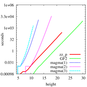
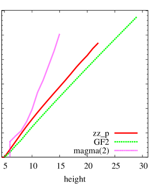
Figure 2: Build time (left) and isomorphism time (right) with respect to tower height. Plot is in logarithmic scale.

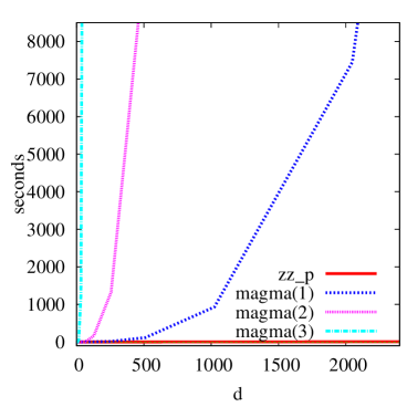
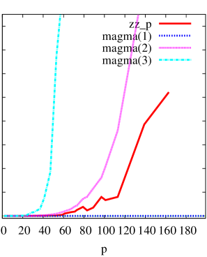
Figure 3: Build times with respect to $d$ (left) and $p$ (right).

The timings of our code are significantly better for increasing height or increasing $d$. Not surprisingly, for increasing $p$, the magma(1) approach performs better than any other: the quo operation simply creates a residue class ring, regardless of the (ir)reducibility of the modulus, so the timing for building two levels barely depend on $p$. Yet, we notice that FAAST has reasonable performances for characteristics up to about $p=50$.

In Tables 1 and 2 we provide some comparative timings for the different arithmetic operations provided by FAAST. The column “Primitive” gives the time taken to build one level of the primitive tower (this includes the precomputation of the data as described in Subsection 4.4); the other entries are self-explanatory. Product and inversion are just wrappers around NTL routines: in these operations we didn’t observe any overhead compared to the native NTL code. All the operations stay within a factor of $30$ of the cost of multiplication, which is satisfactory.

level	Primitive	Push-d.	Lift-up	Product	Inverse	apply $\sigma^{-1}$	apply $\sigma$
19	1.061	0.269	1.165	0.038	0.599	0.572	1.152
20	2.381	0.538	2.554	0.076	1.430	1.146	2.333
21	5.284	1.083	5.645	0.171	3.331	2.306	4.807
22	11.747	2.202	12.595	0.430	7.730	4.811	10.051
23	26.441	4.654	28.641	0.961	18.059	10.240	21.494

Table 1: Some timings in seconds for arithmetics in a generic tower built over $\mathbb{F}_{2}$ using GF2.

level	Primitive	Push-d.	Lift-up	Product	Inverse	apply $\sigma^{-1}$	apply $\sigma$
18	9.159	0.514	8.278	0.321	6.432	2.379	6.624
19	21.695	1.130	20.388	1.083	14.929	6.289	18.202
20	49.137	3.058	48.605	2.444	33.986	10.716	32.493
21	122.252	7.476	123.369	5.307	92.827	26.437	76.780
22	275.110	15.832	279.338	10.971	210.680	47.956	134.167

Table 2: Some timings in seconds for arithmetics in a generic tower built over $\mathbb{F}_{2}$ using zz_p.

Finally, we mention the cost of precomputation. The precomputation of the images of $\sigma$ as explained in Section 6 is quite expensive; most of it is spent computing pseudotraces. Indeed it took one week to precompute the data in Figure 2 (right), while all the other data can be computed in a few hours. There is still space for some minor improvement in FAAST, mainly tweaking recursion thresholds and implementing better algorithms for small and moderate input sizes. Still, we think that only a major algorithmic improvement could consistently speed up this phase.

Isogeny algorithm.

An isogeny is a regular map between two elliptic curves $\mathscr{E}$ and $\mathscr{E}^{\prime}$ that is also a group morphism. In cryptology, isogenies are used in the Schoof-Elkies-Atkin point-counting algorithm BlSeSm99 , but also in more recent constructions RoSt06 ; Teske06 , and the fast computation of isogenies remains a difficult challenge.

Our interest here is Couveignes’ isogeny algorithm Couveignes96 , which computes isogenies of degree $\sim p^{k}$; the algorithm relies on the interpolation of a rational function at special points in an Artin-Schreier tower. The original algorithm in Couveignes96 was first implemented in Lercier97 ; Couveignes’ later paper Couveignes00 described improvements to speed up the computation, but as we already mentioned, a key component, fast arithmetic in Artin-Schreier towers, was still missing. The recent paper DeFeo10 combines this paper’s algorithms and other improvements to achieve a completely explicit version of Couveignes00 .

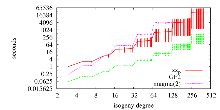
Figure 4: Timings for the isogeny algorithm. Isogenies of degree increasing degree are computed between curves defined over $\mathbb{F}_{2^{101}}$.

The algorithm is composed of 5 phases:

1. Depending on the degree $\ell$ of the isogeny to be computed, a parameter $k$ is chosen such that $p^{k-1}(p-1)>4\ell-2$;

2. a primitive tower of height $\sim k$ is computed (the precise height depends on $\mathscr{E}$ and $\mathscr{E^{\prime}}$, in the example of figure 4 it is always equal to $k-2$);

3. an Artin-Schreier tower in which the $p^{k}$-torsion points of $\mathscr{E}$ are defined is computed and an isomorphism is constructed to the primitive tower;

4. an Artin-Schreier tower in which the $p^{k}$-torsion points of $\mathscr{E^{\prime}}$ are defined is computed and an isomorphism is constructed to the primitive tower;

5. a mapping from $\mathscr{E}[p^{k}]$ to $\mathscr{E^{\prime}}[p^{k}]$ is computed through interpolation;

6. all the possible mappings from $\mathscr{E}[p^{k}]$ to $\mathscr{E^{\prime}}[p^{k}]$ are computed through modular composition until one is found that yields an isogeny.

We ran experiments for curves defined over the base field $\mathbb{F}_{2^{101}}$ for increasing isogeny degree. Figure 4 shows the timings for two implementations of DeFeo10 based on FAAST and one implementation of the same algorithm based on the magma(2) approach; remark that the time scale is logarithmic. The running time is probabilistic because step 6 stops as soon as it has found an isogeny; we plot the average running times with bars around them for minimum/maximum times; the distribution is uniform. Note that the plot in the original ISSAC ’09 version of this paper shows timings that are one order of magnitude worse. This was due to a bug that has later been fixed.

degree	step 2	step 3	step 5	step 6
				preconditioning	avg # iterations	iteration
3	0.008	0.053	0.124	0.005	8	0
5	0.004	0.161	0.310	0.019	16	0.002
11	0.008	0.469	0.749	0.096	32	0.001
17	0.014	1.312	1.779	0.227	64	0.003
37	0.039	3.544	4.168	1.130	128	0.013
67	0.078	9.306	9.651	6.107	256	0.052
131	0.189	23.79	22.124	34.652	512	0.207
257	0.383	59.82	50.532	200.980	1024	0.812

Table 3: Comparative timings for each phase of the isogeny algorithm using GF2.

Table 3 shows comparative timings for each phase of the algorithm. The reason why we left step 4 out of the table is that it is essentially the same as step 3 and timings are nearly identical. Step 6 is asymptotically the most expensive one; it uses some preconditioning to speed up each iteration of the loop. From the point of view of this paper, the most interesting steps are 2-5 since they are the only ones that make use of the library FAAST.

For $p=2$, it should be noted that Lercier’s isogeny algorithm Lercier96 has better performance; for generic, small, $p$ we mention as well a new algorithm by Lercier and Sirvent LeSi09 . See DeFeo10 for further discussions on isogeny computation.

References

• (1) A. Bostan, G. Lecerf, and É. Schost. Tellegen’s principle into practice. In ISSAC’03, pages 37–44. ACM, 2003.
• (2) I. Blake, G. Seroussi, and N. Smart. Elliptic curves in cryptography. Cambridge University Press, 1999.
• (3) W. Bosma, J. Cannon, C. Playoust. The Magma algebra system. I. The user language. J. Symb. Comp., 24(3-4):235-265, 1997.
• (4) R. P. Brent. On computing factors of cyclotomic polynomials. Math. Comp. 61:131–149, 1993.
• (5) R. Brent, P. Gaudry, E. Thomé, P. Zimmermann. Faster multiplication in GF$(2)[x]$. In ANTS’08, 153-166. Springer, 2008.
• (6) P. Bürgisser, M. Clausen, and A. Shokrollahi. Algebraic complexity theory. Springer–Verlag, 1997.
• (7) D. G. Cantor. On arithmetical algorithms over finite fields. Journal of Combinatorial Theory, Series A 50, 285-300, 1989.
• (8) J.-M. Couveignes. Computing $\ell$-isogenies using the $p$-torsion. in ANTS’II, 59–65. Springer, 1996.
• (9) J.-M. Couveignes. Isomorphisms between Artin-Schreier towers. Math. Comp. 69(232): 1625–1631, 2000.
• (10) L. De Feo. Fast algorithms for computing isogenies between ordinary elliptic curves in small characteristic. Preprint, 2010.
• (11) L. De Feo and É. Schost. Fast arithmetical in Artin-Schreier towers over finite fields. in ISSAC’09, pages 127–134. ACM, 2010.
• (12) A. Enge and F. Morain, Fast decomposition of polynomials with known Galois group. in AAECC-15, 254–264. Springer, 2003.
• (13) J. von zur Gathen and J. Gerhard. Modern Computer Algebra. Cambridge University Press, 1999.
• (14) J. von zur Gathen and V. Shoup. Computing Frobenius maps and factoring polynomials Comput. Complexity, vol. 2, 187–224, 1992.
• (15) J. von zur Gathen and J. Gerhard, Arithmetic and factorization of polynomials over $\mathbb{F}_{2}$. In ISSAC’96, pages 1–9. ACM, 1996.
• (16) J. von zur Gathen and V. Shoup. Computing Frobenius maps and factoring polynomials. Comp. Complex., 2(3):187–224, 1992.
• (17) D. Hachenberger, Finite Fields, Normal Bases and Completely Free Elements. Kluwer, 1997.
• (18) E. Kaltofen. Challenges of symbolic computation: my favorite open problems. J. Symb. Comp., 29(6):891–919, 2000.
• (19) K. S. Kedlaya and C. Umans Fast modular composition in any characteristic in FOCS’08, 146–155, IEEE, 2008
• (20) R. Lercier. Computing isogenies in GF($2^{n}$). In ANTS-II, LNCS vol 1122, pages 197–212. Springer, 1996.
• (21) R. Lercier. Algorithmique des courbes elliptiques dans les corps finis. Ph.D. Thesis, École polytechnique, 1997.
• (22) R. Lercier, T. Sirvent. On Elkies subgroups of $\ell$-torsion points in curves defined over a finite field. To appear in J. Théor. Nombres Bordeaux.
• (23) X. Li, M. Moreno Maza, and É. Schost. Fast arithmetic for triangular sets: from theory to practice. In ISSAC’07, pages 269–276. ACM, 2007.
• (24) R. Lidl and H. Niederreiter. Finite Fields, second edition. Cambridge University Press, 1997.
• (25) T. Mateer. Fast Fourier transform algorithms with applications. Ph.D. Thesis, Clemson University, August 2008.
• (26) C. Pascal and É. Schost. Change of order for bivariate triangular sets. In ISSAC’06, pages 277–284. ACM, 2006.
• (27) A. Rostovtsev and A. Stolbunov. Public-key cryptosystem based on isogenies. Cryptology ePrint Archive, Report 2006/145.
• (28) F. Rouillier. Solving zero-dimensional systems through the Rational Univariate Representation. Appl. Alg. in Eng. Comm. Comput., 9(5):433–461, 1999.
• (29) V. Shoup. NTL: A library for doing number theory. http://www.shoup.net/ntl/.
• (30) V. Shoup. Fast construction of irreducible polynomials over finite fields. J. Symb. Comp. 17:371-391, 1994.
• (31) V. Shoup. Efficient computation of minimal polynomials in algebraic extensions of finite fields. In ISSAC’99, pages 53–58, ACM, 1999.
• (32) E. Teske. An elliptic trapdoor system. Journal of Cryptology, 19(1):115–133, 2006.
• (33) Y. Wang and X. Zhu. A Fast Algorithm for Fourier Transform Over Finite Fields and its VLSI Implementation. IEEE Journal on Selected Areas in Communications, 6 (3):572-7, 1988.