10.1080/14786435.20xx.xxxxxx \issn1478-6443 \issnp1478-6435 \jvol00 \jnum00 \jyear2010

Magnetic-field-induced chiral hidden order in $\bm{{\rm URu_{2}Si_{2}}}$

P. Kotetesa โˆ— โˆ—Corresponding author. Email: panagiotis.kotetes@kit.edu โ€ƒโ€ƒ A. Aperisb and G. Varelogiannisc
aInstitut fรผr Theoretische Festkรถrperphysik and DFG-Center for Functional Nanostructures (CFN), Karlsruhe Institute of Technology, 76128 Karlsruhe, Germany
bDepartment of Physics and Astronomy, Uppsala University, Box 516, SE-75120 Uppsala, Sweden
cDepartment of Physics, National Technical University of Athens, GR-15780 Athens, Greece
Abstract

Two of the most striking and yet unresolved manifestations of the hidden order (HO) in ${\rm URu_{2}Si_{2}}$, are associated on one hand with the double-step metamagnetic transitions and on the other with the giant anomalous Nernst signal. Both are observed when a magnetic field is applied along the c-axis. Here we provide for the first time a unified understanding of these puzzling phenomena and the related field-temperature (${\cal B}-T$) phase diagram. We demonstrate that the HO phase at finite fields can be explained with a chiral $d_{xy}+id_{x^{2}-y^{2}}$ spin density wave, assuming that the zero field HO contains only the time-reversal symmetry preserving $id_{x^{2}-y^{2}}$ component. We argue that the presence of the field-induced chiral HO can be reflected in a distinctive non-linear ${\cal B}$-dependence of the Kerr angle, when a Kerr experiment is conducted for finite fields. This fingerprint can be conclusive for the possible emergence of chirality in the HO.


keywords:
${\rm URu_{2}Si_{2}}$; hidden order; chirality; itinerant metamagnetism; anomalous Nernst effect; polar Kerr effect.

1 Introduction

The โ€˜hiddenโ€™ order (HO) transition of heavy fermion ${\rm URu_{2}Si_{2}}$ [1] attracted enormous attention due to the mismatch of its specific heat jump at To=17.5K and the concomitant c-axis oriented tiny antiferromagnetic moment $0.03\mu_{B}/U$, of wave-vector $\bm{Q}_{0}=(0,0,1)$ [2, 3]. This incompatibility has raised great controversy on whether the genuine spin-dipolar antiferromagnetic moment inferred from the Bragg reflection at $\bm{Q}_{0}$ [4], may be the driving order parameter of this transition. In fact, NMR measurements [5, 6] and Larmor diffraction [7], suggest that antiferromagnetism is inhomogeneous and parasitic in the HO phase. In addition, experiments have found no evidence for higher spin-correlators [8].

Inelastic neutron scattering (INS) measurements [9, 10, 11, 12, 13], have revealed two gapped spin excitations at the wave-vectors $\bm{Q}=(1,0,0)$ (equivalent to $\bm{Q}_{0}$) and $\bm{Q}_{1}=(1\pm 0.4,0,0)$. Specifically, the first resonance always accompanies the HO phase and disappears in the pressure-induced large moment antiferromagnetic (LMAF) phase [12, 13] of ${\rm URu_{2}Si_{2}}$. In stark contrast, the second persists and acquires a larger gap upon effecting pressure. Moreover, the emergence of incommensurate excitations can be only understood within an itinerant picture [11], clearly contradicting the predictions of a number of theoretical models, solely based on the localized nature of the U-5f electrons [14, 15, 16, 17, 18]. The itinerant perspective [19, 20, 21, 22, 23, 24, 25, 26, 27, 28, 29, 30, 31] is also supported by the existence of strong Fermi surface nesting at $\bm{Q}_{1}^{\phantom{{\dagger}}}$ [23, 32] and the recent verification of Fermi surface gapping in Angularly Resolved Photoemission Spectroscopy (ARPES) experiments [33, 34].

Under strong external magnetic fields applied along the c-axis and at sufficiently low temperature, ${\rm URu_{2}Si_{2}}$ exhibits a cascade of transitions from the HO to a multitude of unidentified phases that bear similarities with the HO [35, 36]. The sharpest of these transitions are from the HO to a re-entrant HO (RHO) phase around 35T and to a polarized paramagnetic phase near 39T. These are accompanied by double-step itinerant metamagnetism, i.e. two first order jumps in the magnetization; one entering and another one leaving the RHO regime [36]. At elevated temperatures, the transitions become second order, signalling the presence of a metamagnetic critical end point (MCEP) in the ${\cal B}-T$ phase diagram of this material. This intricate behavior, is reminiscent to the case of ${\rm Sr_{3}Ru_{2}O_{7}}$ [37], a prototypical itinerant metamagnet, thus providing further support for the importance of itinerant electron physics in the HO phase.

Apart from the remarkable changes in the phase diagram of the HO, transport measurements under applied magnetic fields inside the HO have revealed that this compound is characterized by an anomalous thermoelectric behaviour up to 35T [38, 39], where the HO has been considered to collapse [39]. The arising Nernst signal has a positive sign and a giant magnitude of several ${\rm\mu V/K}$, while the temperature evolution of the Nernst response resembles to a โ€˜tilted-hillโ€™, demonstrating a peak at about 3-4K, where it reaches the value of $30{\rm\mu V/K}$ for ${\cal B}\simeq 12$T. Up to now, the enhanced Nernst signal has been solely viewed as the signature of the semi-metallic character of this electron-hole compensated metal [38, 39].

Here, we propose that the HO in the ${\cal B}-T$ phase diagram of ${\rm URu_{2}Si_{2}}$ is a chiral $d_{xy}+id_{x^{2}-y^{2}}$ spin density wave (d-SDW) phase. Within a mean-field approximation we reproduce self-consistently the experimentally resolved ${\cal B}-T$ phase diagram of this compound. Moreover, we provide a unified explanation for the emergence of characteristic phenomena that accompany the HO phase such as the puzzling metamagnetism [36, 35] and the giant Nernst signal [38, 39]. In addition, we propose a Kerr angle measurement in the presence of an external magnetic field, that could directly identify the formation of a chiral HO in this compound, through the non-linear ${\cal B}$-dependence associated with the induced chirality. Note that our proposal is also compatible with the chiral superconducting state that is believed to appear within the HO [40].

2 Mean-field description of the field induced chiral d-SDW HO

The particular $d_{xy}+id_{x^{2}-y^{2}}$ momentum structure of the order parameter is considered here to originate from repulsive nearest and next-nearest inter-site Coulomb interactions of the form โˆ‘๐’Šโ‰ ๐’‹V๐’Šโ€‹๐’‹โ€‹n๐’Šโ€‹n๐’‹subscript๐’Š๐’‹superscriptsubscript๐‘‰๐’Š๐’‹absentsuperscriptsubscript๐‘›๐’Šabsentsuperscriptsubscript๐‘›๐’‹absent\sum_{\bm{i}\neq\bm{j}}V_{\bm{i}\bm{j}}^{\phantom{{\dagger}}}n_{\bm{i}}^{\phantom{{\dagger}}}n_{\bm{j}}^{\phantom{{\dagger}}}, while it is described by a two component c-axis polarized spin-triplet order parameter $\Delta^{z}(\bm{k})=\Delta_{1}\sin k_{x}\sin k_{y}-i\Delta_{2}(\cos k_{x}-\cos k_{y})$, with the second of them bearing similarities to orbital orders already proposed for URu2Si2 [19, 20, 21, 22, 28, 27]. The additional $d_{xy}$ component renders the HO chiral rather than orbital, violating time-reversal symmetry in a macroscopic level due to the development of an intrinsic orbital ferromagnetic moment. It has been shown, that due to this orbital magnetic-field-coupling, any unconventional density wave of the form $id_{x^{2}-y^{2}}$ will acquire an additional field-dependent $d_{xy}$ component [41, 42]. Even if the chiral order does not appear in zero-field, it will be necessarily field-induced, affecting the ${\cal B}-T$ phase diagram of the HO and every transport measurement realized in the presence of a field, such as the Nernst effect. In fact, when one of the two components is solely field-induced, the chiral order may be viewed as a magnetic-field-renormalized orbital order (see Appendix). In this sense, our theory is fully compatible with all the earlier proposed orbital-order-based models [19, 20, 21, 22, 28, 27] and it could be considered as a natural and necessary extension to them.

However, the chiral order exhibits properties not familiar to orbital orders. Generally the spontaneous appearance of a chiral phase leads to a polar Kerr effect [43] and the generation of anomalous Hall electric [44] and thermoelectric currents [45, 46], including the โ€˜tilted-hillโ€™ giant Nernst signal recently shown to arise in strongly insulating chiral condensates [46]. In the present case, the chiral HO will be field-induced and it will manifest its presence in all the phenomena mentioned above through the characteristic non-linear field-dependence of the $d_{xy}$ order parameter.

3 Metamagnetism within our self-consistently extracted magnetic field-temperature phase diagram
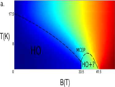
The resulting โ„ฌโˆ’Tโ„ฌ๐‘‡{\cal B}-T phase diagram is depicted in Fig.ย 1a,b. We observe that our phase diagram grasps to a large extent both qualitative and quantitative features of the experimental observations [36, 35]. At โ„ฌ=0โ„ฌ0{\cal B}=0T, ฮ”1=0subscriptฮ”10\Delta_{1}=0 and ฮ”2=1.55โ€‹meVsubscriptฮ”21.55meV\Delta_{2}=1.55{\rm meV}. The latter order parameter corresponds to the
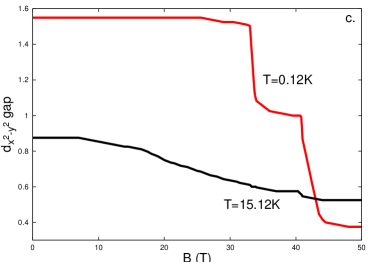
 iโ€‹dx2โˆ’y2๐‘–subscript๐‘‘superscript๐‘ฅ2superscript๐‘ฆ2id_{x^{2}-y^{2}} component which as we observe in Fig.ย 1c, slightly decreases upon raising the magnetic field for low temperatures. In contrast, the dxโ€‹ysubscript๐‘‘๐‘ฅ๐‘ฆd_{xy} order parameter ฮ”1subscriptฮ”1\Delta_{1}, rises monotonically. A MCEP [37] (MCEP) is located at โ„ฌcโ€‹1=33.5subscriptโ„ฌ๐‘133.5{\cal B}_{c1}=33.5T and Tโ‰ƒsimilar-to-or-equals\simeq3K, down to which the driving HO gap, ฮ”2subscriptฮ”2\Delta_{2}, evolves continuously with the magnetic field satisfying the quadratic relation ฮ”2โ€‹(โ„ฌz)/ฮ”2โ€‹(0)โ‰ƒ1โˆ’(โ„ฌz/โ„ฌcโ€‹1)2similar-to-or-equalssubscriptฮ”2subscriptโ„ฌ๐‘งsubscriptฮ”201superscriptsuperscriptsubscriptโ„ฌ๐‘งabsentsuperscriptsubscriptโ„ฌ๐‘1absent2\Delta_{2}({\cal B}_{z})/\Delta_{2}(0)\simeq 1-({\cal B}_{z}^{\phantom{{\dagger}}}/{\cal B}_{c1}^{\phantom{{\dagger}}})^{2}. This behaviour has been verified in magnetoresistance measurements [47]. In stark contrast, ฮ”2subscriptฮ”2\Delta_{2} remains practically constant for temperatures below the MCEP which could explain the field independent energy scale witnessed in the inelastic magnetic response at ๐‘ธ1subscript๐‘ธ1\bm{Q}_{1} [10], in terms of the spin exciton scenario [25]. A continuous evolution with the field is not compatible with the first-order character of the metamagnetic step. This property can settle the controversy concerning the observed field dependence of the HO.

Refer to captionRefer to captionRefer to captionRefer to captionRefer to caption
Figure 1: a. Self-consistently extracted โ„ฌโˆ’Tโ„ฌ๐‘‡{\cal B}-T phase diagram of the chiral d-spin density wave. The chiral HO is present in the whole phase diagram. The reduced 
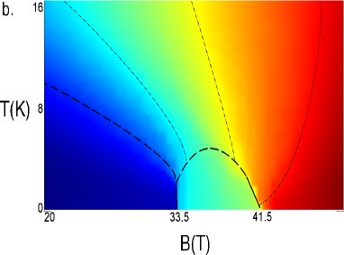
magnitude of the order parameters in the high field and temperature regions, mask its presence providing a thermodynamic phase boundary (dashed lines). b. A Metamagnetic Critical End Point (MCEP) is located at Tโ‰ƒ3similar-to-or-equals๐‘‡3T\simeq 3K and โ„ฌ=โ„ฌcโ€‹1=33.5โ„ฌsubscriptโ„ฌ๐‘133.5{\cal B}={\cal B}_{c1}=33.5T. Two metamagnetic steps appear at โ„ฌcโ€‹1=33.5subscriptโ„ฌ๐‘133.5{\cal B}_{c1}=33.5T and โ„ฌcโ€‹1โ‰ƒ41similar-to-or-equalssubscriptโ„ฌ๐‘141{\cal B}_{c1}\simeq 41T along with the formation of crossover areas (separated by dash-dotted lines), in agreement with the experimental observations [36, 35]. c. For T<<3K, the dx2โˆ’y2subscript๐‘‘superscript๐‘ฅ2superscript๐‘ฆ2d_{x^{2}-y^{2}} order parameter is nearly constant until โ„ฌ=โ„ฌcโ€‹1โ„ฌsubscriptโ„ฌ๐‘1{\cal B}={\cal B}_{c1}, where it abruptly decreases. This is presumably the gap seen in neutron scattering experiments [10]. Above the MCEP, the gap evolves smoothly with the field, explaining the dependence arising from bulk measurements [47]. The saturation appearing 
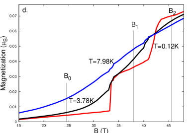
in high fields does not give rise to any thermodynamic anomaly, rendering the chiral HO experimentally undetectable. d. The metamagnetic steps are accompanied by an abrupt 
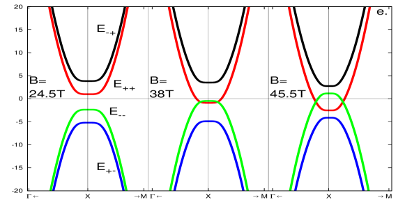
increase of the magnetization. For higher temperatures the first order character becomes milder leading to a smooth evolution. e. The cascade of the metamagnetic transitions, appears due to additional band crossings at each โ„ฌcsubscriptโ„ฌ๐‘{\cal B}_{c} [48]. The reconstruction of the Fermi surface increases steeply the carriers of the system and concomitantly the magnetization.

Our self-consistent phase diagram exhibits double-step metamagnetism (Fig.ย 1d) at ${\cal B}_{c1}$=33.5T and ${\cal B}_{c2}\simeq$41T, below 3K in agreement with experiments [36, 35]. Note that the occurrence of metamagnetism in such a high field scale is also related to the appearance of the $d_{xy}$ component, which leads to an enhancement of the critical temperature of the dominant $d_{x^{2}-y^{2}}$ order parameter (see Appendix). The gradual increment of the field shifts the four quasiparticle bands through the combined orbital-Zeeman coupling (see Eq.11). At each ${\cal B}_{c}$ an additional energy branch crosses the Fermi level (Fig.ย 1e) providing an abrupt increase to the density of carriers of the system and a concomitant steep enhancement of the magnetization [48]. For higher temperatures the first order character of the metamagnetic steps becomes milder, leading to a smoother increase of the magnetization in this region of fields.

The pronounced similaritities presented in our phase diagram compared to Ref.ย [36, 35], are accompanied by important ramifications arising from the finite chirality of the order parameter. First and more importantly, the chiral HO is present in the whole diagram, due to the enhanced critical temperature, originating from the orbital magnetic-field coupling. For magnetic fields ${\cal B}_{c1}<{\cal B}<{\cal B}_{c2}$, both order parameters of the chiral phase suffer a severe decrease in their magnitude. Consequently, the chiral $d_{xy}+id_{x^{2}-y^{2}}$ phase is still present in this region but unavoidably masked due to the destruction of its topological rigidity. The HO persists even for ${\cal B}\geq{\cal B}_{c2}$, behaving as a polarized paramagnetic metal.

Despite of the continuous presence of the chiral HO, the emergence of the MCEP may lead to the generation of novel phases at ${\cal B}_{c1}$, that could coexist with the chiral HO, constituting phases ${\rm III,V}$ of Ref. [35]. It has been shown that under quite generic conditions, the effect of a Zeeman field on a charge density wave can lead to a field-induced SDW transition and vice versa [48, 49]. In this sense, the magnetic field permits a number of possible induced phases [50, 51] such as the chiral spin singlet d-density wave phase, studied in the context of high-Tc superconductors [43, 52, 45, 42, 46], or even the spin singlet and triplet electron nematic phases [24, 53, 54, 55, 56].

4 Giant Nernst signal and anomalous thermoelectricity
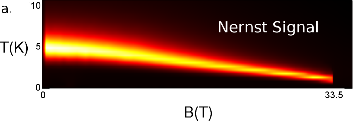
Refer to captionRefer to captionRefer to caption
Figure 2: a. โ„ฌโˆ’Tโ„ฌ๐‘‡{\cal B}-T dependence of the self-consistently calculated Nernst signal. The arising Nernst response presents a large positive signal, of about one order larger than the experimentally observed [38]. The giant response originates from the topological robustness of the chiral phase [46]. The field destruction of the Nernst signal at โ„ฌcโ€‹1subscriptโ„ฌ๐‘1{\cal B}_{c1} agrees with the experiment [39], although here, it is accompanied by the dramatic reduction, rather than the
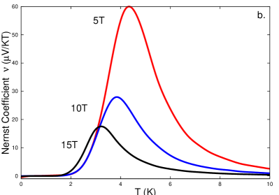
 collapse of the dxโ€‹y,dx2โˆ’y2subscript๐‘‘๐‘ฅ๐‘ฆsubscript๐‘‘superscript๐‘ฅ2superscript๐‘ฆ2d_{xy},d_{x^{2}-y^{2}} order parameters. b. The Nernst coefficient ฮฝ=N/โ„ฌz๐œˆ๐‘subscriptโ„ฌ๐‘ง\nu=N/{\cal B}_{z} shows a โ€˜tilted-hillโ€™ profile, with a pronounced peak in the region 3-5K 
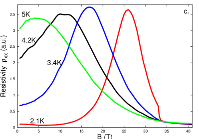
following the experimental data [38]. c. Field dependence of the resistivity for several temperatures. For T<To๐‘‡subscript๐‘‡๐‘œT<T_{o}, the presence of a โ€˜kinkโ€™, also found in experiments [39], may be naturally attributed to the field-enhancement of the dxโ€‹ysubscript๐‘‘๐‘ฅ๐‘ฆd_{xy} component.

By taking into account both topological and quasiparticle contributions in computing the electric ($\sigma_{xx},\sigma_{xy}$) and thermoelectric conductivity ($\alpha_{xx},\alpha_{xy}$) tensor elements, we demonstrate that the Nernst response in the HO phase can be understood in terms of the chiral $d_{xy}+id_{x^{2}-y^{2}}$ HO parameter. Using the values of the order parameters providing the phase diagram of Fig.ย 1, we obtain a giant Nernst signal, that has a magnitude of about one order larger than the one observed in the experiments [57]. The origin of the โ€˜tilted-hillโ€™ Nernst signal is directly related to the chirality and the strong Fermi surface gapping. As presented in Ref.ย [46], the strong insulating character of the chiral HO phase forces the thermopower and the Nernst signal to become equal at a thermoelectric crossing point. In the vicinity of this point, the usually large values of the thermopower also imply a Nernst signal of the same magnitude, leading unavoidably to an enhancement of the latter. However, the thermoelectric rigitity and the tendency towards a giant Nernst signal are lost exactly at ${\cal B}_{c1}$. The steep decrease of the $d_{x^{2}-y^{2}}$ gap across this first order transition and the concomitant Fermi surface reconstruction which partially destroys the insulating properties of the phase, lead to the full supression of the response (Fig.ย 2a) in accordance with Ref.ย [39].

Furthermore, the Nernst coefficient exhibits a peaked structure with temperature and decreases upon raising the magnetic field already at 10K (Fig.ย 2b). Notice that although this phase is also present even above 17.5K, it does not lead to a large Nernst signal, becoming in this manner experimentally elusive. We have also calculated the resistivity for finite fields and temperatures. We observe in Fig.ย 2c that the field dependence of the resistivity exhibits a kink with the increase of the magnetic field. This is a definite fingerprint of the field induced $d_{xy}$ component and coincides with the experimental findings [39]. This kink shifts to lower magnetic fields upon raising temperature, since the $d_{xy}$ gap gradually weakens.

5 Prediction of a non-linear ${\cal B}$-dependence for the Kerr angle due to the induced chirality

To verify our scenario we propose the measurement of the Kerr angle [43] in the presence of a static magnetic field. This type of measurement is an ideal probe of the possible emergence of chirality in the HO phase [58]. The field-induced chiral HO will provide the dominant contribution to the Kerr angle. More importantly, we expect that the arising Kerr angle $\vartheta_{K}^{\phantom{{\dagger}}}$ will exhibit a distinctive magnetic field dependence when the sample is cooled down and heated up again in the presence of a static external magnetic field (Fig.ย 3). The Kerr angle [58, 43, 59] is defined as

$\displaystyle\vartheta_{K}^{\phantom{{\dagger}}}=\frac{4\pi}{n(n^{2}-1)da^{2}}\frac{\sigma_{xy}^{\Im}(\omega)}{\omega}\,,$ (1)

where $n$ is the refractive index, $d$ is the c-axis thickness of the sample, $a=5{\AA}$ the in plane lattice constant and $\sigma_{xy}^{\Im}$ the imaginary part of the dynamical Hall conductivity. In the low field regime (${\cal B}\leq 20T$), the dynamical Hall conductivity is dominated by the chirality contribution. For a Sagnac inteferometer [58] $\hbar\omega=0.8eV=6420{\rm cm^{-1}}$ and $\lambda=1550{\rm nm}$, while the plasma frequency of ${\rm URu_{2}Si_{2}}$ is $\hbar\omega_{p}=2131{\rm cm^{-1}}\simeq 266{\rm meV}$ [60]. The refractive index in this case is defined as $n=\sqrt{1-\left(\omega_{p}/\omega\right)^{2}}$. Since $\omega>>\omega_{p}$ we may use the approximation $n\simeq 1$ and $n^{2}-1=-\left(\omega_{p}/\omega\right)^{2}$. We find that the Kerr angle is equal to

$\displaystyle\vartheta_{K}^{\phantom{{\dagger}}}({\cal B},T)$ $\displaystyle=$ $\displaystyle\frac{4\pi}{n(n^{2}-1)da^{2}}\frac{\sigma_{xy}^{\Im}(\omega)}{\omega}\simeq-\frac{2}{n(n^{2}-1)}\frac{e^{2}}{\hbar c}\frac{\lambda}{d}\frac{\Delta_{1}({\cal B},T)}{\hbar\omega}$ (2)
$\displaystyle=$ $\displaystyle-2\frac{e^{2}}{\hbar c}\frac{\lambda}{d}\frac{\Delta_{1}({\cal B},T)}{\hbar\omega_{p}}\left(\frac{\omega}{\omega_{p}}\right)\,.$
Refer to caption
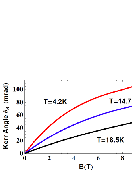
Figure 3: Predicted magnetic field dependence of the Kerr angle due to the magnetic induction of the chiral HO. The emergence of the chiral d-SDW yields a large field-induced Kerr angle. The latter can be observed only for finite magnetic fields, and even above $T_{o}$, due to the increase of the HO critical temperature arising from the magnetic induction of the $d_{xy}$ order parameter (see Appendix). Starkingly, for low temperatures we obtain a characteristic non-linear ${\cal B}$-dependence which can identify the emergence of the field-induced chiral HO proposed here.

By taking into account the value of the fine structure constant $e^{2}/\hbar c=1/137$ and by setting $d\simeq 2{\rm nm}$, we obtain a rough estimation of the Kerr angle as $\vartheta_{K}^{\phantom{{\dagger}}}\simeq 128\Delta_{1}{\rm mrad}$ with $\Delta_{1}$ in ${\rm meV}$. The maximum value of $\Delta_{1}$ is equal to $1.5{\rm meV}$, which defines an upper bound $\vartheta_{K}^{\phantom{{\dagger}}}\leq 190{\rm mrad}$. The magnitude of the Kerr angle demonstrates that the expected response is very large and easily detectable. The observation of the particular non-linear ${\cal B}$-dependent chirality contribution to the Kerr angle, as opposed to the linearly dependent quasiparticle contribution, constitutes a sharp signature of our magnetic-field-induced chiral HO scenario, unveiling its possible connection to the intricate ${\rm URu_{2}Si_{2}}$ phenomenology.

6 Summary and conclusions

In conclusion, assuming that the zero-field HO in ${\rm URu_{2}Si_{2}}$ is an unconventional $id_{x^{2}-y^{2}}$ spin density wave phase that preserves TRS, we have demonstrated that both the giant anomalous Nernst signal and the double-step metamagnetism observed in the HO of this material can be understood in a unified way, in terms of a magnetic field-induced $d_{xy}$ component which renders the HO chiral in finite magnetic fields. This chiral HO is characterized by a finite orbital ferromagnetic moment (arising from a finite Berry curvature) which ensures a robust giant anomalous Nernst signal. At the same time, the interplay of orbital and Zeeman moments allow for a sequential softening of the emergent four quasiparticle branches by the magnetic field, leading to double-step metamagnetism.

Within a mean-field theory for the magnetic field-induced chiral HO, while taking fully into account effects of induced orbital moment in the chiral phase, we have numerically obtained the ${\cal B}-T$ phase diagram of this material. For the same set of numerical self-consistent data, we have shown that also the temperature profile of the obtained Nernst signal matches that of the relevant experiments. In order to unveil the chiral nature of the HO, we propose a Kerr effect experiment in the presence of an external magnetic field. We predict a characteristic temperature and magnetic field profile of the Kerr angle. If the latter is indeed observed, this would open a new perspective to our understanding of the HO in ${\rm URu_{2}Si_{2}}$.

Acknowledgements

We are indebted to J. Mydosh, P. M. Oppeneer, Y. Matsuda, K. Behnia and A. Kapitulnik for illuminating discussions. This work was partially funded by ฮ โ€‹EVEฮ EVE{\rm\Pi EVE} by NTU Athens. A. A. wishes to thank the organizers of the Workshop on Hidden Order, Superconductivity and Magnetism in ${\rm URu_{2}Si_{2}}$, Lorentz Center, Leiden for their hospitality.

References

  • [1] Mydosh J. A. and Oppeneer P. M., Rev. Mod. Phys. 83 (2011) p.1301.
  • [2] Palstra T. T. M. et al., Phys. Rev. Lett. 55 (1985) p.2727.
  • [3] Schlabitz W. et al., Z. Phys. B 62 (1986) p.171.
  • [4] Walker M. B. et al., Phys. Rev. Lett. 71 (1993) p.2630.
  • [5] Amitsuka H., and Yokoyama M., Physica B 452 (2003) p.329.
  • [6] Takagi S. et al., J. Phys. Soc. Jpn. 76 (2007) p.033708.
  • [7] Niklowitz P. G. et al., Phys. Rev. Lett. 104 (2010) p.106406.
  • [8] Mason T. E. et al., J. Phys.: Condens. Matter. 7 (1995) p.5089.
  • [9] Broholm C. et al., Phys. Rev. Lett. 58 (1987) p.1467.
  • [10] Bourdarot F., Fak B., Habicht K., and Prokes K., Phys. Rev. Lett. 90 (2003) p.067203.
  • [11] Wiebe C. R. et al., Nature Physics 3 (2007) p.1.
  • [12] Villaume A. et al., Phys. Rev. B 78 (2008) p.012504.
  • [13] Aoki D. et al., J. Phys. Soc. Jpn. 78 (2009) p.053701.
  • [14] Santini P. and Amoretti G., Phys. Rev. Lett. 73 (1994) p.1027.
  • [15] Barzykin V. and Gorโ€™kov L. P., Phys. Rev. Lett. 74 (1995) p.4301.
  • [16] Kiss A. and Fazekas P., Phys. Rev. B 71 (2005) p.054415.
  • [17] Haule K., and Kotliar G., Nature Physics 5 (2009) p.796.
  • [18] Chandra P., Coleman P. and Flint R., Nature 493 (2013) p.621.
  • [19] Ramirez A. P. et al., Phys. Rev. Lett. 68 (1992) p.2680.
  • [20] Ikeda H., and Ohashi Y., Phys. Rev. Lett. 81 (1998) p.3723.
  • [21] Chandra P., Coleman P., Mydosh J. A., and Tripathi V., Nature 417 (2002) p.831.
  • [22] Virosztek A., Maki K., Dora B., Int. J. Mod. Phys. B 16 (2002) p.1667.
  • [23] Elgazzar S. et al., Nature Materials 8 (2009) p.337.
  • [24] Varma C. M. and Zhu L., Phys. Rev. Lett. 96 (2006) p.036405.
  • [25] Balatsky A. V. et al., Phys. Rev. B 79 (2009) p.214413.
  • [26] Cricchio F., Bultmark F., Grรฅnรคs O. and Nordstrรถm L., Phys. Rev. Lett. 103 (2009) p.107202.
  • [27] Oppeneer P. M. et al., Phys. Rev. B 84 (2011) p.241102(R).
  • [28] Fujimoto S., Phys. Rev. Lett. 106 (2011) p.196407.
  • [29] Das T., Sci. Rep. 2 (2012) p.596.
  • [30] Riseborough P.S., Coqblin B. and Magalhรฃes S.G., Phys. Rev. B 85 (2012) p.165116.
  • [31] Ikeda H. et al., Nature Physics 8 (2012) p.528.
  • [32] Oppeneer P. M. et al., Phys. Rev. B 82 (2010) p.205103.
  • [33] Santander-Syro F. et al., Nature Physics 5 (2009) p.637.
  • [34] Meng J.-Q. et al., Phys. Rev. Lett. 111 (2013) p.127002.
  • [35] Kim K. H. et al., Phys. Rev. Lett. 91 (2003) p.256401.
  • [36] Harrison N., Jaime M., and Mydosh J. A., Phys. Rev. Lett. 90 (2003) p.096402.
  • [37] Grigera S. A. et al., Science 294 (2001) p.329.
  • [38] Bel R. et al., Phys. Rev. B 70 (2004) p.220501.
  • [39] Levallois J. et al., Europhys. Lett. 85 (2009) p.27003.
  • [40] Kasahara Y. et al., Phys. Rev. Lett. 99 (2007) p.116402.
  • [41] Zhu J.-X., and Balatsky A. V., Phys. Rev. B 65 (2002) p.132502.
  • [42] Kotetes P., and Varelogiannis G., Phys. Rev. B 80 (2009) p.212401.
  • [43] Tewari S., Zhang C., Yakovenko V. M., and Das Sarma S., Phys. Rev. Lett. 100 (2008) p.217004.
  • [44] Kotetes P., and Varelogiannis G., Europhys. Lett. 84 (2008) p.37012.
  • [45] Zhang C., Tewari S., Yakovenko V. M., and Das Sarma S., Phys. Rev. B 78 (2008) p.174508.
  • [46] Kotetes P., and Varelogiannis G., Phys. Rev. Lett. 104 (2010) p.106404.
  • [47] Mentink S. A. M. et al., Phys. Rev. B 53 (1996) p.6014.
  • [48] Aperis A., Varelogiannis G. and Littlewood P. B., J. Phys.: Conf. Ser. 150 (2009) p.042007.
  • [49] Aperis A. et al., Europhys. Lett. 83 (2008) p.67008.
  • [50] Tsonis S., Kotetes P., Varelogiannis G. and Littlewood P.B., J. Phys.: Condens. Matter 20 (2008) p.434234.
  • [51] Varelogiannis G., arXiv:1305.2976.
  • [52] Kotetes P., and Varelogiannis G., Phys. Rev. B 78 (2008) p.220509.
  • [53] Yamase H., and Kohno H., J. Phys. Soc. Jpn. 69 (2000) p.332.
  • [54] Halboth C. J., and Metzner W., Phys. Rev. Lett. 85 (2000) p.5162.
  • [55] Wu C., Sun K., Fradkin E., and Zhang S.-C., Phys. Rev. B 75 (2007) p.115103.
  • [56] Sun K., and Fradkin E., Phys. Rev. B 78 (2008) p.245122.
  • [57] Matsuda Y., talk given at the Workshop on Hidden Order, Superconductivity and Magnetism in ${\rm URu_{2}Si_{2}}$, Lorentz Center, Leiden 2013.
  • [58] Kapitulnik A. et al., New J. Phys. 11 (2009) p.055060.
  • [59] Mineev V. P., Phys. Rev. B 76 (2007) p.212501.
  • [60] Degiorgi L. et al., Z. Phys. B 102 (1997) p.367.
\appendices

7 Mean-field decoupling and order parameter symmetries

Based on the phenomenology of ${\rm URu_{2}Si_{2}}$, we assume that in the real material, the chiral d-SDW orders at the incommensurate wave vector $\bm{Q}_{1}=(1\pm 0.4,0,0)$. However, describing microscopically a chiral order parameter with this ordering wave-vector, demands taking into account the main four Fermi lines that give rise to this nesting symmetry [1, 2]. This is a very complex and unnecessary task since our results do not depend on the microscopic details of the model. Our results concerning the anomalous Hall thermoelectric transport are based solely on the topological content and the symmetry properties of this phase. Moreover, the phase diagram and the metamagnetic transitions are also based on the general principles of itinerant metamagnetism, according to which this phenomenon originates from band crossing [3]. Under these conditions it is permissible to consider a simplified single-band tight-binding model characterized by the nesting condition $\varepsilon(\bm{k}+\bm{Q})=-\varepsilon(\bm{k})=-[-2t(\cos k_{x}+\cos k_{y})]$ with the commensurate nesting wave-vector $\bm{Q}=(\pi,\pi)$. This condition, should stand in a similar way for the real bands of URu2Si2, and within our approximate simple model we simulate this situation. Finally, within this framework we consider the $d$-wave harmonics $\Delta_{1}^{\phantom{{\dagger}}}(\bm{k})=\Delta_{1}^{\phantom{{\dagger}}}\sin k_{x}\sin k_{y}$, $\Delta_{2}^{\phantom{{\dagger}}}(\bm{k})=\Delta_{2}^{\phantom{{\dagger}}}(\cos k_{x}-\cos k_{y})$ with $\Delta_{1,2}^{\phantom{{\dagger}}}=\Delta^{*}_{1,2}$.

To study the phase diagram of the chiral d-SDW phase we consider that it is driven by an a inter-site Coulomb repulsion including nearest and next-nearest neighbours

$\displaystyle{\cal V}_{int}^{\phantom{{\dagger}}}$ $\displaystyle=$ โˆ’1vโ€‹โˆ‘๐’Œ,๐’Œโ€ฒโˆ‘s,sโ€ฒVโ€‹(๐’Œโˆ’๐’Œโ€ฒ)โ€‹c๐’Œ,sโ€ โ€‹c๐’Œ+๐‘ธ,sโ€ฒโ€‹c๐’Œโ€ฒ+๐‘ธ,sโ€ฒโ€ โ€‹c๐’Œโ€ฒ,s1๐‘ฃsubscript๐’Œsuperscript๐’Œโ€ฒsubscript๐‘ superscript๐‘ โ€ฒ๐‘‰๐’Œsuperscript๐’Œโ€ฒsuperscriptsubscript๐‘๐’Œ๐‘ โ€ superscriptsubscript๐‘๐’Œ๐‘ธsuperscript๐‘ โ€ฒabsentsuperscriptsubscript๐‘superscript๐’Œโ€ฒ๐‘ธsuperscript๐‘ โ€ฒโ€ superscriptsubscript๐‘superscript๐’Œโ€ฒ๐‘ absent\displaystyle-\frac{1}{v}\sum_{\bm{k},\bm{k}^{\prime}}\sum_{s,s^{\prime}}V(\bm{k}-\bm{k}^{\prime})c_{\bm{k},s}^{{\dagger}}c_{\bm{k}+\bm{Q},s^{\prime}}^{\phantom{{\dagger}}}c_{\bm{k}^{\prime}+\bm{Q},s^{\prime}}^{{\dagger}}c_{\bm{k}^{\prime},s}^{\phantom{{\dagger}}}\phantom{.} (3)

with s,sโ€ฒ=โ†‘,โ†“formulae-sequence๐‘ superscript๐‘ โ€ฒโ†‘โ†“s,s^{\prime}=\uparrow,\downarrow and $V(\bm{q})=2V^{\prime}(\cos q_{x}+\cos q_{y})+4V^{\prime\prime}\cos q_{x}\cos q_{y}$. The momenta $\bm{k},\bm{k}^{\prime}$ belong to the whole Brillouin zone (${\cal B.Z.}$) if $\bm{Q}$ is incommensurate and in the reduced Brillouin zone if $\bm{Q}$ is commensurate satisfying $\bm{k}+2\bm{Q}=\bm{k}$. The potential is separable providing $V(\bm{k}-\bm{k}^{\prime})=\sum_{n}V_{n}^{\phantom{{\dagger}}}f_{n}^{\phantom{{\dagger}}}({\bm{k}})f_{n}^{\phantom{{\dagger}}}({\bm{k}^{\prime}})$ with $n=1,2,..,8$ corresponding to the form factors $f_{n}(\bm{k}):\cos k_{x}\pm\cos k_{y}$, $\sin k_{x}\pm\sin k_{y}$, $\cos k_{x}\cos k_{y}$, $\sin k_{x}\sin k_{y}$, $\cos k_{x}\sin k_{y}$, $\sin k_{x}\cos k_{y}$ with the driving potentials $V_{n}^{\phantom{{\dagger}}}=V^{\prime}$ for $n=1,2,3,4$ and $V_{n}^{\phantom{{\dagger}}}=4V^{\prime\prime}$ for the rest. Then within a mean-field treatment we introduce the staggered order parameters

ฮ”๐‘ธsโ€‹sโ€‹(๐’Œ)superscriptsubscriptฮ”๐‘ธ๐‘ ๐‘ ๐’Œ\displaystyle\Delta_{\bm{Q}}^{ss}(\bm{k}) $\displaystyle=$ โˆ’1vโ€‹โˆ‘๐’Œโ€ฒVโ€‹(๐’Œโˆ’๐’Œโ€ฒ)โ€‹โŸจc๐’Œโ€ฒ+๐‘ธ,sโ€ โ€‹c๐’Œโ€ฒ,sโŸฉ=โˆ‘nฮ”๐‘ธ,nsโ€‹sโ€‹(๐’Œ)s=โ†‘,โ†“formulae-sequence1๐‘ฃsubscriptsuperscript๐’Œโ€ฒ๐‘‰๐’Œsuperscript๐’Œโ€ฒdelimited-โŸจโŸฉsuperscriptsubscript๐‘superscript๐’Œโ€ฒ๐‘ธ๐‘ โ€ superscriptsubscript๐‘superscript๐’Œโ€ฒ๐‘ absentsubscript๐‘›superscriptsubscriptฮ”๐‘ธ๐‘›๐‘ ๐‘ ๐’Œ๐‘ โ†‘โ†“\displaystyle-\frac{1}{v}\sum_{\bm{k}^{\prime}}V(\bm{k}-\bm{k}^{\prime})\left<c_{\bm{k}^{\prime}+\bm{Q},s}^{{\dagger}}c_{\bm{k}^{\prime},s}^{\phantom{{\dagger}}}\right>=\sum_{n}\Delta_{\bm{Q},n}^{ss}(\bm{k})\quad s=\uparrow,\downarrow (4)

and the corresponding irreducible $\bm{k}$-independent staggered order parameters

ฮ”๐‘ธ,nsโ€‹ssuperscriptsubscriptฮ”๐‘ธ๐‘›๐‘ ๐‘ \displaystyle\Delta_{\bm{Q},n}^{ss} $\displaystyle=$ โˆ’1vโ€‹โˆ‘๐’ŒVnโ€‹fnโ€‹(๐’Œ)โ€‹โŸจc๐’Œ+๐‘ธ,sโ€ โ€‹c๐’Œ,sโŸฉs=โ†‘,โ†“.formulae-sequence1๐‘ฃsubscript๐’Œsuperscriptsubscript๐‘‰๐‘›absentsuperscriptsubscript๐‘“๐‘›absent๐’Œdelimited-โŸจโŸฉsuperscriptsubscript๐‘๐’Œ๐‘ธ๐‘ โ€ superscriptsubscript๐‘๐’Œ๐‘ absent๐‘ โ†‘โ†“\displaystyle-\frac{1}{v}\sum_{\bm{k}}V_{n}^{\phantom{{\dagger}}}f_{n}^{\phantom{{\dagger}}}(\bm{k})\left<c_{\bm{k}+\bm{Q},s}^{{\dagger}}c_{\bm{k},s}^{\phantom{{\dagger}}}\right>\quad s=\uparrow,\downarrow\,. (5)

The interaction decouples in the following way

$\displaystyle{\cal V}_{int}^{\phantom{{\dagger}}}$ $\displaystyle=$ โˆ‘๐’Œ{ฮ”๐‘ธโ†‘โ†‘(๐’Œ)c๐’Œ,โ†‘โ€ c๐’Œ+๐‘ธ,โ†‘+ฮ”๐‘ธโ†“โ†“(๐’Œ)c๐’Œ,โ†“โ€ c๐’Œ+๐‘ธ,โ†“+h.c.}+vโˆ‘n,s|ฮ”๐‘ธ,nsโ€‹s|2Vn,\displaystyle\sum_{\bm{k}}\left\{\Delta_{\bm{Q}}^{\uparrow\uparrow}(\bm{k})c_{\bm{k},\uparrow}^{{\dagger}}c_{\bm{k}+\bm{Q},\uparrow}^{\phantom{{\dagger}}}+\Delta_{\bm{Q}}^{\downarrow\downarrow}(\bm{k})c_{\bm{k},\downarrow}^{{\dagger}}c_{\bm{k}+\bm{Q},\downarrow}^{\phantom{{\dagger}}}+h.c.\right\}+v\sum_{n,s}\frac{|\Delta_{\bm{Q},n}^{ss}|^{2}}{V_{n}^{\phantom{{\dagger}}}}\,,\qquad (6)

with $v$ the volume of the corresponding ${\cal B.Z.}$. By introducing the spinor ฮจ๐’Œโ€ =(c๐’Œ,โ†‘โ€ โ€‹c๐’Œ,โ†“โ€ โ€‹c๐’Œ+๐‘ธ,โ†‘โ€ โ€‹c๐’Œ+๐‘ธ,โ†“โ€ )superscriptsubscriptฮจ๐’Œโ€ superscriptsubscript๐‘๐’Œโ†‘โ€ superscriptsubscript๐‘๐’Œโ†“โ€ superscriptsubscript๐‘๐’Œ๐‘ธโ†‘โ€ superscriptsubscript๐‘๐’Œ๐‘ธโ†“โ€ \Psi_{\bm{k}}^{{\dagger}}=(c_{\bm{k},\uparrow}^{{\dagger}}\phantom{{\dagger}}c_{\bm{k},\downarrow}^{{\dagger}}\phantom{{\dagger}}c_{\bm{k}+\bm{Q},\uparrow}^{{\dagger}}\phantom{{\dagger}}c_{\bm{k}+\bm{Q},\downarrow}^{{\dagger}}) and by using the isospin and spin Pauli matrices ฯ„i,sisubscript๐œ๐‘–subscript๐‘ ๐‘–\tau_{i},s_{i} with $i=1,2,3$ complemented by the related unit matrices ฯ„0,s0superscriptsubscript๐œ0absentsuperscriptsubscript๐‘ 0absent\tau_{0}^{\phantom{{\dagger}}},s_{0}^{\phantom{{\dagger}}}, we furnish a representation of the $4\times 4$ mean-field hamiltonian as Kronecker products of the form ฯ„ฮผโŠ—sฮฝtensor-productsubscript๐œ๐œ‡superscriptsubscript๐‘ ๐œˆabsent\tau_{\mu}\otimes s_{\nu}^{\phantom{{\dagger}}} where $\mu,\nu=0,1,2,3$ (for simplicity we omit $\otimes$). The most general chiral d-SDW state is defined as $\Delta_{\bm{Q}}^{z}(\bm{k})=\Delta_{1}^{\phantom{{\dagger}}}(\bm{k})-i\Delta_{2}^{\phantom{{\dagger}}}(\bm{k})$. Moreover we introduce the kinetic term of the paramagnetic state โ„‹0=โˆ‘๐’Œ,s{(ฮตโ€‹(๐’Œ)โˆ’ฮผ)โ€‹c๐’Œ,sโ€ โ€‹c๐’Œ,s+(ฮตโ€‹(๐’Œ+๐‘ธ)โˆ’ฮผ)โ€‹c๐’Œ+๐‘ธ,sโ€ โ€‹c๐’Œ+๐‘ธ,s}superscriptsubscriptโ„‹0absentsubscript๐’Œ๐‘ ๐œ€๐’Œ๐œ‡superscriptsubscript๐‘๐’Œ๐‘ โ€ superscriptsubscript๐‘๐’Œ๐‘ absent๐œ€๐’Œ๐‘ธ๐œ‡superscriptsubscript๐‘๐’Œ๐‘ธ๐‘ โ€ superscriptsubscript๐‘๐’Œ๐‘ธ๐‘ absent{\cal H}_{0}^{\phantom{{\dagger}}}=\sum_{\bm{k},s}\left\{(\varepsilon(\bm{k})-\mu)c_{\bm{k},s}^{{\dagger}}c_{\bm{k},s}^{\phantom{{\dagger}}}+(\varepsilon(\bm{k}+\bm{Q})-\mu)c_{\bm{k}+\bm{Q},s}^{{\dagger}}c_{\bm{k}+\bm{Q},s}^{\phantom{{\dagger}}}\right\} along with a chemical potential $\mu$. Putting together all these terms and using the fact that in the spin-triplet state $\Delta_{\bm{Q}}^{z}=\Delta_{\bm{Q}}^{\uparrow\uparrow}=-\Delta_{\bm{Q}}^{\downarrow\downarrow}$, we obtain the quasiparticle Hamiltonian

$\displaystyle{\cal H}_{q-p}^{\phantom{{\dagger}}}$ $\displaystyle=$ โˆ‘๐’Œฮจ๐’Œโ€ {ฮ”1โ€‹(๐’Œ)+ฮ”1โˆ—โ€‹(๐’Œ)2ฯ„1s3+ฮ”1โ€‹(๐’Œ)โˆ’ฮ”1โˆ—โ€‹(๐’Œ)2iฯ„2s3\displaystyle\sum_{\bm{k}}\Psi_{\bm{k}}^{{\dagger}}\Bigl{\{}\frac{\Delta_{1}^{\phantom{{\dagger}}}(\bm{k})+\Delta_{1}^{*}(\bm{k})}{2}\tau_{1}^{\phantom{{\dagger}}}s_{3}^{\phantom{{\dagger}}}+\frac{\Delta_{1}^{\phantom{{\dagger}}}(\bm{k})-\Delta_{1}^{*}(\bm{k})}{2}i\tau_{2}^{\phantom{{\dagger}}}s_{3}^{\phantom{{\dagger}}} (7)
$\displaystyle-$ iโ€‹ฮ”2โ€‹(๐’Œ)โˆ’ฮ”2โˆ—โ€‹(๐’Œ)2โ€‹ฯ„1โ€‹s3+ฮ”2โ€‹(๐’Œ)+ฮ”2โˆ—โ€‹(๐’Œ)2โ€‹ฯ„2โ€‹s3๐‘–subscriptฮ”2๐’Œsuperscriptsubscriptฮ”2๐’Œ2superscriptsubscript๐œ1absentsuperscriptsubscript๐‘ 3absentsubscriptฮ”2๐’Œsuperscriptsubscriptฮ”2๐’Œ2superscriptsubscript๐œ2absentsuperscriptsubscript๐‘ 3absent\displaystyle i\frac{\Delta_{2}(\bm{k})-\Delta_{2}^{*}(\bm{k})}{2}\tau_{1}^{\phantom{{\dagger}}}s_{3}^{\phantom{{\dagger}}}+\frac{\Delta_{2}(\bm{k})+\Delta_{2}^{*}(\bm{k})}{2}\tau_{2}^{\phantom{{\dagger}}}s_{3}^{\phantom{{\dagger}}}
$\displaystyle+$ $\displaystyle\frac{\varepsilon(\bm{k})+\varepsilon(\bm{k}+\bm{Q})}{2}\tau_{0}^{\phantom{{\dagger}}}s_{0}^{\phantom{{\dagger}}}+\frac{\varepsilon(\bm{k})-\varepsilon(\bm{k}+\bm{Q})}{2}\tau_{3}^{\phantom{{\dagger}}}s_{0}^{\phantom{{\dagger}}}-\mu\tau_{0}^{\phantom{{\dagger}}}s_{0}^{\phantom{{\dagger}}}\Bigl{\}}\Psi_{\bm{k}}^{\phantom{{\dagger}}}\,,$

and the elastic energy needed to build up the two density wave gaps

$\displaystyle{\cal H}_{\bm{\Delta}^{2}}^{\phantom{{\dagger}}}=2v\left(\frac{|\Delta_{1}|^{2}}{4V^{\prime\prime}}+\frac{|\Delta_{2}|^{2}}{V^{\prime}}\right)\,.$ (8)

8 Intrinsic orbital moment and magnetic field coupling

With these definitions we may write the quasiparticle hamiltonian in the condensed form โ„‹qโˆ’p=โˆ‘๐’Œฮจ๐’Œโ€ โ€‹{๐’ˆ^โ€‹(๐’Œ)โ‹…๐‰โˆ’ฮผ}โ€‹ฮจ๐’Œsuperscriptsubscriptโ„‹๐‘ž๐‘absentsubscript๐’Œsuperscriptsubscriptฮจ๐’Œโ€ โ‹…^๐’ˆ๐’Œ๐‰๐œ‡superscriptsubscriptฮจ๐’Œabsent{\cal H}_{q-p}^{\phantom{{\dagger}}}=\sum_{\bm{k}}\Psi_{\bm{k}}^{{\dagger}}\left\{\widehat{\bm{g}}(\bm{k})\cdot\bm{\tau}-\mu\right\}\Psi_{\bm{k}}^{\phantom{{\dagger}}} where we have introduced the vector ๐’ˆ^โ€‹(๐’Œ)=(ฮ”1โ€‹(๐’Œ)โ€‹s3,ฮ”2โ€‹(๐’Œ)โ€‹s3,ฮตโ€‹(๐’Œ)โ€‹s0)^๐’ˆ๐’Œsubscriptฮ”1๐’Œsuperscriptsubscript๐‘ 3absentsubscriptฮ”2๐’Œsuperscriptsubscript๐‘ 3absent๐œ€๐’Œsuperscriptsubscript๐‘ 0absent\widehat{\bm{g}}(\bm{k})=\left(\Delta_{1}(\bm{k})s_{3}^{\phantom{{\dagger}}},\Delta_{2}(\bm{k})s_{3}^{\phantom{{\dagger}}},\varepsilon(\bm{k})s_{0}^{\phantom{{\dagger}}}\right). Diagonalizing the above hamiltonian yields the eigenstates |ฮฆs,ฮฝโ€‹(๐’Œ)โŸฉketsubscriptฮฆ๐‘ ๐œˆ๐’Œ|\Phi_{s,\nu}(\bm{k})\rangle with energy dispersions Es,ฮฝโ€‹(๐’Œ)=โˆ’ฮผ+ฮฝโ€‹Eโ€‹(๐’Œ)subscript๐ธ๐‘ ๐œˆ๐’Œ๐œ‡๐œˆ๐ธ๐’ŒE_{s,\nu}(\bm{k})=-\mu+\nu E(\bm{k}) and ฮฝ=ยฑ,s=โ†‘,โ†“formulae-sequence๐œˆplus-or-minus๐‘ โ†‘โ†“\nu=\pm,s=\uparrow,\downarrow, $E(\bm{k})=|\widehat{\bm{g}}(\bm{k})|=\sqrt{\varepsilon^{2}(\bm{k})+|\Delta_{\bm{Q}}^{z}(\bm{k})|^{2}}$. The non trivial topological content of this Hamiltonian generates a non zero $U(1)$ Berry connection [4] ๐“s,ฮฝโ€‹(๐’Œ)=โŸจฮฆs,ฮฝโ€‹(๐’Œ)โˆฃiโ€‹โˆ‡๐’Œโˆฃฮฆs,ฮฝโ€‹(๐’Œ)โŸฉsubscript๐“๐‘ ๐œˆ๐’Œquantum-operator-productsubscriptฮฆ๐‘ ๐œˆ๐’Œ๐‘–superscriptsubscriptbold-โˆ‡๐’Œabsentsubscriptฮฆ๐‘ ๐œˆ๐’Œ\bm{{\cal A}}_{s,\nu}(\bm{k})=\langle\Phi_{s,\nu}(\bm{k})\mid i\bm{\nabla}_{\bm{k}}^{\phantom{{\dagger}}}\mid\Phi_{s,\nu}(\bm{k})\rangle and a corresponding Berry curvature defined as ๐›€s,ฮฝโ€‹(๐’Œ)=โˆ‡๐’Œร—๐“s,ฮฝโ€‹(๐’Œ)=ฮฉs,ฮฝzโ€‹(๐’Œ)โ€‹๐’›^subscript๐›€๐‘ ๐œˆ๐’Œsubscriptbold-โˆ‡๐’Œsubscript๐“๐‘ ๐œˆ๐’Œsubscriptsuperscriptฮฉ๐‘ง๐‘ ๐œˆ๐’Œbold-^๐’›\bm{\Omega}_{s,\nu}(\bm{k})=\bm{\nabla}_{\bm{k}}\times\bm{{\cal A}}_{s,\nu}(\bm{k})=\Omega^{z}_{s,\nu}(\bm{k})\bm{\hat{z}}, i.e. oriented along the $z$-axis. The detailed expression for the Berry curvature reads [6, 7, 5, 8]

ฮฉs,ฮฝzโ€‹(๐’Œ)=12โ€‹Tโ€‹rsโ€‹{โˆ’ฮฝโ€‹a22โ€‹E3โ€‹(๐’Œ)โ€‹๐’ˆ^โ€‹(๐’Œ)โ‹…(โˆ‚๐’ˆ^โ€‹(๐’Œ)โˆ‚kxร—โˆ‚๐’ˆ^โ€‹(๐’Œ)โˆ‚ky)}.superscriptsubscriptฮฉ๐‘ ๐œˆ๐‘ง๐’Œ12๐‘‡superscriptsubscript๐‘Ÿ๐‘ absentโ‹…๐œˆsuperscript๐‘Ž22superscript๐ธ3๐’Œ^๐’ˆ๐’Œ^๐’ˆ๐’Œsuperscriptsubscript๐‘˜๐‘ฅabsent^๐’ˆ๐’Œsuperscriptsubscript๐‘˜๐‘ฆabsent\displaystyle\Omega_{s,\nu}^{z}(\bm{k})=\frac{1}{2}Tr_{s}^{\phantom{{\dagger}}}\left\{\frac{-\nu a^{2}}{2E^{3}(\bm{k})}\widehat{\bm{g}}(\bm{k})\cdot\left(\frac{\partial\widehat{\bm{g}}(\bm{k})}{\partial k_{x}^{\phantom{{\dagger}}}}\times\frac{\partial\widehat{\bm{g}}(\bm{k})}{\partial k_{y}^{\phantom{{\dagger}}}}\right)\right\}\,. (9)

We observe that the Berry curvature is not depending on spin while it just changes sign when $\nu=\pm$. The intrinsic orbital moment of this state is straighforward calculated using the definition [4]

๐’Žs,ฮฝโ€‹(๐’Œ)superscriptsubscript๐’Ž๐‘ ๐œˆabsent๐’Œ\displaystyle\bm{m}_{s,\nu}^{\phantom{{\dagger}}}(\bm{k}) $\displaystyle=$ e2โ€‹โ„โ€‹iโ€‹โŸจโˆ‡๐’Œฮฆs,ฮฝโ€‹(๐’Œ)โˆฃร—[โ„‹โ€‹(๐’Œ)โˆ’Es,ฮฝโ€‹(๐’Œ)]โ€‹โˆฃโˆ‡๐’Œฮฆs,ฮฝโ€‹(๐’Œ)โŸฉ๐‘’2Planck-constant-over-2-pi๐‘–brasubscriptbold-โˆ‡๐’Œsuperscriptsubscriptฮฆ๐‘ ๐œˆabsent๐’Œdelimited-[]โ„‹๐’Œsuperscriptsubscript๐ธ๐‘ ๐œˆabsent๐’Œketsubscriptbold-โˆ‡๐’Œsuperscriptsubscriptฮฆ๐‘ ๐œˆabsent๐’Œ\displaystyle\frac{e}{2\hbar i}\langle\bm{\nabla}_{\bm{k}}\Phi_{s,\nu}^{\phantom{{\dagger}}}(\bm{k})\mid\times\left[{\cal H}(\bm{k})-E_{s,\nu}^{\phantom{{\dagger}}}(\bm{k})\right]\mid\bm{\nabla}_{\bm{k}}\Phi_{s,\nu}^{\phantom{{\dagger}}}(\bm{k})\rangle (10)
$\displaystyle=$ eโ€‹ฮฝโ„โ€‹Eโ€‹(๐’Œ)โ€‹๐›€s,ฮฝโ€‹(๐’Œ).๐‘’๐œˆPlanck-constant-over-2-pi๐ธ๐’Œsuperscriptsubscript๐›€๐‘ ๐œˆabsent๐’Œ\displaystyle\frac{e\nu}{\hbar}E(\bm{k})\bm{\Omega}_{s,\nu}^{\phantom{{\dagger}}}(\bm{k})\,.

One may observe that the orbital moment is band independent. When we apply a magnetic field, the system interacts with both the Zeeman and the orbital moment mzโ€‹(๐’Œ)=eโ€‹Eโ€‹(๐’Œ)โ€‹ฮฉs,+zโ€‹(๐’Œ)/โ„subscript๐‘š๐‘ง๐’Œ๐‘’๐ธ๐’Œsuperscriptsubscriptฮฉ๐‘ ๐‘ง๐’ŒPlanck-constant-over-2-pim_{z}(\bm{k})=eE(\bm{k})\Omega_{s,+}^{z}(\bm{k})/\hbar yielding the following interacting Hamiltonian โ„‹โ„ฌโ€‹(๐’Œ)=โˆ’(ฮผBโ€‹ฯ„0โ€‹s3โˆ’mzโ€‹(๐’Œ)โ€‹ฯ„0โ€‹s0)โ€‹โ„ฌsubscriptโ„‹โ„ฌ๐’Œsubscript๐œ‡๐ตsuperscriptsubscript๐œ0absentsuperscriptsubscript๐‘ 3absentsubscript๐‘š๐‘ง๐’Œsuperscriptsubscript๐œ0absentsuperscriptsubscript๐‘ 0absentโ„ฌ{\cal H_{{\cal B}}}(\bm{k})=-(\mu_{B}\tau_{0}^{\phantom{{\dagger}}}s_{3}^{\phantom{{\dagger}}}-m_{z}(\bm{k})\tau_{0}^{\phantom{{\dagger}}}s_{0}^{\phantom{{\dagger}}}){\cal B}. The inclusion of the magnetic coupling leads to the four field dependent eigenenergies:

$\displaystyle E_{s,\nu}^{{\cal B}}(\bm{k})=-[s\mu_{B}-m_{z}(\bm{k})]{\cal B}+\nu\sqrt{\varepsilon^{2}(\bm{k})+|\Delta_{\bm{Q}}^{z}(\bm{k})|^{2}}\ \ ,\ \ \nu,s=\pm$ (11)

corresponding to the conduction and valence bands of the upper and lower spin sectors respectively.

9 Free energy and self-consistency equations

Having set up the microscopic description of the chiral d-SDW condensate, interacting with both Zeeman and the intrisic orbital moments with a magnetic field, we may solve the self-consistency equations that derive from the minimization of the free-energy functional

โ„ฑ=2โ€‹vโ€‹(ฮ”124โ€‹Vโ€ฒโ€ฒ+ฮ”22Vโ€ฒ)โˆ’1ฮฒโ€‹โˆ‘๐’Œ,s,ฮฝlnโก(1+eโˆ’ฮฒโ€‹Es,ฮฝโ„ฌโ€‹(๐’Œ)),โ„ฑ2๐‘ฃsuperscriptsubscriptฮ”124superscript๐‘‰โ€ฒโ€ฒsuperscriptsubscriptฮ”22superscript๐‘‰โ€ฒ1๐›ฝsubscript๐’Œ๐‘ ๐œˆ1superscript๐‘’๐›ฝsuperscriptsubscript๐ธ๐‘ ๐œˆโ„ฌ๐’Œ\displaystyle{\cal F}=2v\left(\frac{\Delta_{1}^{2}}{4V^{\prime\prime}}+\frac{\Delta_{2}^{2}}{V^{\prime}}\right)-\frac{1}{\beta}\sum_{\bm{k},s,\nu}\ln\left(1+e^{-\beta E_{s,\nu}^{{\cal B}}(\bm{k})}\right)\,, (12)

with $t=50{\rm meV}$, $\mu=0.69{\rm meV}$, $\mu_{B}^{\phantom{{\dagger}}}=0.058{\rm meV/T}$, $a=5{\AA}$, $V^{\prime}=23.5{\rm meV}$ and $V^{\prime\prime}=35.25{\rm meV}$. Minimization of the above yields the following two self-consistency equations, that determine the order parameters of the chiral d-SDW [6]

ฮ”i=โˆ’Vi2โ€‹vโ€‹โˆ‘๐’Œ,s,ฮฝ{ฮฝโ€‹ฮ”iโ€‹fi2โ€‹(๐’Œ)2โ€‹Eโ€‹(๐’Œ)+eโ€‹a2โ€‹tโ„โ€‹โ„ฌzโ€‹ฮ”~iโ€‹Sโ€‹(๐’Œ)E2โ€‹(๐’Œ)โ€‹[1โˆ’2โ€‹(ฮ”iโ€‹(๐’Œ)Eโ€‹(๐’Œ))2]}superscriptsubscriptฮ”๐‘–absentsuperscriptsubscript๐‘‰๐‘–absent2๐‘ฃsubscript๐’Œ๐‘ ๐œˆ๐œˆsuperscriptsubscriptฮ”๐‘–absentsuperscriptsubscript๐‘“๐‘–2๐’Œ2๐ธ๐’Œ๐‘’superscript๐‘Ž2๐‘กPlanck-constant-over-2-pisuperscriptsubscriptโ„ฌ๐‘งabsentsuperscriptsubscript~ฮ”๐‘–absent๐‘†๐’Œsuperscript๐ธ2๐’Œdelimited-[]12superscriptsuperscriptsubscriptฮ”๐‘–absent๐’Œ๐ธ๐’Œ2\displaystyle\Delta_{i}^{\phantom{{\dagger}}}=\frac{-V_{i}^{\phantom{{\dagger}}}}{2v}\sum_{\bm{k},s,\nu}\left\{\nu\Delta_{i}^{\phantom{{\dagger}}}\frac{f_{i}^{2}(\bm{k})}{2E(\bm{k})}+\frac{ea^{2}t}{\hbar}{\cal B}_{z}^{\phantom{{\dagger}}}\widetilde{\Delta}_{i}^{\phantom{{\dagger}}}\frac{S(\bm{k})}{E^{2}(\bm{k})}\left[1-2\left(\frac{\Delta_{i}^{\phantom{{\dagger}}}(\bm{k})}{E(\bm{k})}\right)^{2}\right]\right\}
ร—nFโ€‹[Es,ฮฝ๐“‘โ€‹(๐’Œ)],absentsuperscriptsubscript๐‘›๐นabsentdelimited-[]superscriptsubscript๐ธ๐‘ ๐œˆ๐“‘๐’Œ\displaystyle\times n_{F}^{\phantom{{\dagger}}}\left[E_{s,\nu}^{\bm{{\cal B}}}(\bm{k})\right]\,, (13)

with $V_{1}^{\phantom{{\dagger}}}=4V^{\prime\prime}$, $V_{2}^{\phantom{{\dagger}}}=V^{\prime}$, $\widetilde{\Delta}_{1,2}^{\phantom{{\dagger}}}=\Delta_{2,1}^{\phantom{{\dagger}}}$, $S(\bm{k})=\sin^{2}k_{x}\cos^{2}k_{y}+\sin^{2}k_{y}$ and $n_{F}^{\phantom{{\dagger}}}$ the Fermi-Dirac distribution.

10 Landau theory of the magnetic-field-induced chiral d-spin density wave HO and Tc enhancement

In order to understand phenomenologically the mechanism leading to the field-induced chiral HO as this arises microscopically from the previous appendices, we can construct a employ a Landau description. The numerical solution of the equations, points to the following Landau picture for the chiral d-spin density wave order

$\displaystyle{\cal F}=\alpha_{1}^{\phantom{{\dagger}}}\frac{\Delta_{1}^{2}}{2}+\alpha_{2}(T-T_{o}^{\phantom{{\dagger}}})\frac{\Delta_{2}^{2}}{2}+\beta\frac{\Delta_{2}^{4}}{4}-g\Delta_{1}^{\phantom{{\dagger}}}\Delta_{2}^{\phantom{{\dagger}}}{\cal B}_{z}^{\phantom{{\dagger}}}$ (14)

The phenomenological constants $\alpha_{1,2}^{\phantom{{\dagger}}},\beta$ and the field ${\cal B}_{z}^{\phantom{{\dagger}}}$, are positive. The coefficient $\alpha_{1}^{\phantom{{\dagger}}}$ ensures that the $d_{xy}^{\phantom{{\dagger}}}$ component is magnetic-field induced. From the numerical analysis we have discerned that the sign of the orbital coupling $g$, is also positive. With this convention $\Delta_{1,2}^{\phantom{{\dagger}}}$ have the same sign. The mean-field solution for the $\Delta_{1}$ component yields

$\displaystyle\frac{\partial{\cal F}}{\partial\Delta_{1}}=0\Rightarrow\alpha_{1}\Delta_{2}^{\phantom{{\dagger}}}$ $\displaystyle=$ $\displaystyle g\Delta_{2}^{\phantom{{\dagger}}}{\cal B}_{z}\,.$ (15)

One may โ€˜integrate outโ€™ the induced $\Delta_{1}$ component and obtain an effective theory only in terms of the driving $d_{x^{2}-y^{2}}$ order parameter $\Delta_{2}$. This is straightforward, yielding

$\displaystyle{\cal F}_{eff}=\alpha(T-T_{o}^{\phantom{{\dagger}}})\frac{\Delta_{2}^{2}}{2}+\beta\frac{\Delta_{2}^{4}}{4}-\frac{g^{2}}{\alpha_{1}}\Delta_{2}^{2}{\cal B}_{z}^{2}=\alpha\left[T-T_{o}^{\phantom{{\dagger}}}({\cal B}_{z}^{\phantom{{\dagger}}})\right]\frac{\Delta_{2}^{2}}{2}+\beta\frac{\Delta_{2}^{4}}{4}\,.$ (16)

Note, that since $\alpha_{1}>0$, the quadratic magnetic-field-coupling leads to an enhanced critical temperature $T_{o}^{\phantom{{\dagger}}}({\cal B}_{z}^{\phantom{{\dagger}}})=T_{o}^{\phantom{{\dagger}}}+\frac{g^{2}}{\alpha_{1}}{\cal B}_{z}^{2}$ for the $d_{x^{2}-y^{2}}$ component and consequently for the chiral order. In the magnetic-field-induced chiral d-spin density wave, the $\Delta_{2}$ order parameter is driving the transition.

11 Magnetization and thermoelectric response

As far as the magnetic and transport properties are concerned, we have used the expressions found in the theory of orbital magnetization [4]. The magnetization is the summation of both spin and orbital contributions in the following way โ„ณzโ„ฌ=โ„ณz,sโ€‹pโ€‹iโ€‹nโ„ฌ+โ„ณz,oโ€‹rโ€‹bโ„ฌsuperscriptsubscriptโ„ณ๐‘งโ„ฌsuperscriptsubscriptโ„ณ๐‘ง๐‘ ๐‘๐‘–๐‘›โ„ฌsuperscriptsubscriptโ„ณ๐‘ง๐‘œ๐‘Ÿ๐‘โ„ฌ{\cal M}_{z}^{\cal B}={\cal M}_{z,spin}^{\cal B}+{\cal M}_{z,orb}^{\cal B} where:

โ„ณz,sโ€‹pโ€‹iโ€‹nโ„ฌsuperscriptsubscriptโ„ณ๐‘ง๐‘ ๐‘๐‘–๐‘›โ„ฌ\displaystyle{\cal M}_{z,spin}^{\cal B} $\displaystyle=$ 1vโ€‹โˆ‘๐’Œ,s,ฮฝ{(1+eโ€‹โ„ฌโ€‹a2โ„โ€‹ฮฉs,ฮฝzโ€‹(๐’Œ))โ€‹ฮผBโ€‹sโ€‹nFโ€‹[Es,ฮฝโ„ฌโ€‹(๐’Œ)]}1๐‘ฃsubscript๐’Œ๐‘ ๐œˆ1๐‘’โ„ฌsuperscript๐‘Ž2Planck-constant-over-2-pisuperscriptsubscriptฮฉ๐‘ ๐œˆ๐‘ง๐’Œsuperscriptsubscript๐œ‡๐ตabsent๐‘ superscriptsubscript๐‘›๐นabsentdelimited-[]superscriptsubscript๐ธ๐‘ ๐œˆโ„ฌ๐’Œ\displaystyle\frac{1}{v}\sum_{\bm{k},s,\nu}\left\{\left(1+\frac{e{\cal B}a^{2}}{\hbar}\Omega_{s,\nu}^{z}(\bm{k})\right)\mu_{B}^{\phantom{{\dagger}}}s\phantom{.}n_{F}^{\phantom{{\dagger}}}[E_{s,\nu}^{\cal B}(\bm{k})]\right\} (17)
$\displaystyle{\cal M}_{z,orb}^{\cal B}$ $\displaystyle=$ $\displaystyle\frac{1}{v}\sum_{\bm{k},s,\nu}\Biggl{\{}\left(1+\frac{e{\cal B}a^{2}}{\hbar}\Omega_{s,\nu}^{z}(\bm{k})\right)m_{z}(\bm{k})n_{F}^{\phantom{{\dagger}}}[E_{s,\nu}^{\cal B}(\bm{k})]$ (18)
$\displaystyle+$ $\displaystyle\frac{ea^{2}}{\hbar}\Omega_{s,\nu}^{z}(\bm{k})k_{B}T\ln\left(1+e^{-E_{s,\nu}^{\cal B}(\bm{k})/k_{B}T}\right)\Biggl{\}}\,.$

The above expressions include the Berry phase correction to the electronic density of states, as this is apparent from the factor (1+eโ€‹โ„ฌโ€‹a2โ„โ€‹ฮฉs,ฮฝzโ€‹(๐’Œ))1๐‘’โ„ฌsuperscript๐‘Ž2Planck-constant-over-2-pisuperscriptsubscriptฮฉ๐‘ ๐œˆ๐‘ง๐’Œ\left(1+\frac{e{\cal B}a^{2}}{\hbar}\Omega_{s,\nu}^{z}(\bm{k})\right) in the first equation.

For transport properties, we have taken into account both topological $(\sigma_{xy,top}^{\cal B}$, $\alpha_{xy,top}^{\cal B})$ and quasiparticle contributions ($\sigma_{xy,q-p}^{\cal B}$, $\alpha_{xy,q-p}^{\cal B})$ in calculating the Hall transport, while we have incorporated the Berry phase corrections in the scattering time and density states of the system. We have used ฯ„s,ฮฝโ€‹(๐’Œ)โ‰กฯ„=3.3โ‹…10โˆ’13โ€‹ssubscript๐œ๐‘ ๐œˆ๐’Œ๐œโ‹…3.3superscript1013๐‘ \tau_{s,\nu}(\bm{k})\equiv\tau=3.3\cdot 10^{-13}s. Based on experimental data [9] $m^{*}=25m_{e}$, and $\omega_{c}\tau({\cal B}=1T)=0.08$, the estimated scattering time is of the order of 10โˆ’12โ€‹ssuperscript1012๐‘ 10^{-12}s. In order to illustrate the chirality induced giant Nernst signal, we have on purpose selected a 3 times smaller relaxation time so to demonstrate that the possible enhancement of the quasiparticle contribution due to a large $\tau$, is not crucial for the anomalous Hall thermoelectricity. In finite magnetic fields, the initially constant relaxation time, becomes field and momentum dependent in the following manner: ฯ„s,ฮฝโ„ฌโ€‹(๐’Œ)=ฯ„1+eโ„โ€‹โ„ฌโ€‹ฮฉs,ฮฝzโ€‹(๐’Œ)superscriptsubscript๐œ๐‘ ๐œˆโ„ฌ๐’Œ๐œ1๐‘’Planck-constant-over-2-piโ„ฌsuperscriptsubscriptฮฉ๐‘ ๐œˆ๐‘ง๐’Œ\tau_{s,\nu}^{\cal B}(\bm{k})=\frac{\tau}{1+\frac{e}{\hbar}{\cal B}\Omega_{s,\nu}^{z}(\bm{k})}. The electric and thermoelectric coefficients read:

$\displaystyle\sigma_{xx}^{\cal B}$ $\displaystyle=$ โˆ’1vโ€‹โˆ‘๐’Œ,s,ฮฝnFโ€ฒโ€‹[Es,ฮฝโ„ฌโ€‹(๐’Œ)]1+eโ„โ€‹โ„ฌโ€‹ฮฉs,ฮฝzโ€‹(๐’Œ)โ€‹(ฯ„s,ฮฝโ„ฌโ€‹(๐’Œ)โ„)โ€‹[vs,ฮฝx,โ„ฌโ€‹(๐’Œ)]2,1๐‘ฃsubscript๐’Œ๐‘ ๐œˆsuperscriptsubscript๐‘›๐นโ€ฒdelimited-[]superscriptsubscript๐ธ๐‘ ๐œˆโ„ฌ๐’Œ1๐‘’Planck-constant-over-2-piโ„ฌsuperscriptsubscriptฮฉ๐‘ ๐œˆ๐‘ง๐’Œsuperscriptsubscript๐œ๐‘ ๐œˆโ„ฌ๐’ŒPlanck-constant-over-2-pisuperscriptdelimited-[]superscriptsubscript๐‘ฃ๐‘ ๐œˆ๐‘ฅโ„ฌ๐’Œ2\displaystyle-\frac{1}{v}\sum_{\bm{k},s,\nu}\frac{n_{F}^{\prime}\left[E_{s,\nu}^{\cal B}({\bm{k}})\right]}{1+\frac{e}{\hbar}{\cal B}\Omega_{s,\nu}^{z}(\bm{k})}\left(\frac{\tau_{s,\nu}^{\cal B}(\bm{k})}{\hbar}\right)\left[v_{s,\nu}^{x,\cal B}(\bm{k})\right]^{2}\,,
$\displaystyle\alpha_{xx}^{\cal B}$ $\displaystyle=$ +1vโ€‹โˆ‘๐’Œ,s,ฮฝnFโ€ฒโ€‹[Es,ฮฝโ„ฌโ€‹(๐’Œ)]1+eโ„โ€‹โ„ฌโ€‹ฮฉs,ฮฝzโ€‹(๐’Œ)โ€‹(ฯ„s,ฮฝโ„ฌโ€‹(๐’Œ)โ„)โ€‹[vs,ฮฝx,โ„ฌโ€‹(๐’Œ)]2โ€‹(Es,ฮฝโ„ฌโ€‹(๐’Œ)kBโ€‹T),1๐‘ฃsubscript๐’Œ๐‘ ๐œˆsuperscriptsubscript๐‘›๐นโ€ฒdelimited-[]superscriptsubscript๐ธ๐‘ ๐œˆโ„ฌ๐’Œ1๐‘’Planck-constant-over-2-piโ„ฌsuperscriptsubscriptฮฉ๐‘ ๐œˆ๐‘ง๐’Œsuperscriptsubscript๐œ๐‘ ๐œˆโ„ฌ๐’ŒPlanck-constant-over-2-pisuperscriptdelimited-[]superscriptsubscript๐‘ฃ๐‘ ๐œˆ๐‘ฅโ„ฌ๐’Œ2superscriptsubscript๐ธ๐‘ ๐œˆโ„ฌ๐’Œsuperscriptsubscript๐‘˜๐ตabsent๐‘‡\displaystyle+\frac{1}{v}\sum_{\bm{k},s,\nu}\frac{n_{F}^{\prime}\left[E_{s,\nu}^{\cal B}({\bm{k}})\right]}{1+\frac{e}{\hbar}{\cal B}\Omega_{s,\nu}^{z}(\bm{k})}\left(\frac{\tau_{s,\nu}^{\cal B}(\bm{k})}{\hbar}\right)\left[v_{s,\nu}^{x,\cal B}(\bm{k})\right]^{2}\left(\frac{E_{s,\nu}^{\cal B}(\bm{k})}{k_{B}^{\phantom{{\dagger}}}T}\right)\,,
$\displaystyle\sigma_{xy,top}^{\cal B}$ $\displaystyle=$ โˆ’1vโ€‹โˆ‘๐’Œ,s,ฮฝnFโ€‹[Es,ฮฝโ„ฌโ€‹(๐’Œ)]โ€‹ฮฉs,ฮฝzโ€‹(๐’Œ),1๐‘ฃsubscript๐’Œ๐‘ ๐œˆsuperscriptsubscript๐‘›๐นabsentdelimited-[]superscriptsubscript๐ธ๐‘ ๐œˆโ„ฌ๐’Œsuperscriptsubscriptฮฉ๐‘ ๐œˆ๐‘ง๐’Œ\displaystyle-\frac{1}{v}\sum_{\bm{k},s,\nu}n_{F}^{\phantom{{\dagger}}}[E_{s,\nu}^{\cal B}({\bm{k}})]\Omega_{s,\nu}^{z}(\bm{k})\,,
$\displaystyle\alpha_{xy,top}^{\cal B}$ $\displaystyle=$ +1vโ€‹โˆ‘๐’Œ,s,ฮฝ{(Es,ฮฝโ„ฌโ€‹(๐’Œ)kBโ€‹T)โ€‹nFโ€‹[Es,ฮฝโ„ฌโ€‹(๐’Œ)]+lnโก(1+eโˆ’Es,ฮฝโ„ฌโ€‹(๐’Œ)/kBโ€‹T)}โ€‹ฮฉs,ฮฝzโ€‹(๐’Œ),1๐‘ฃsubscript๐’Œ๐‘ ๐œˆsuperscriptsubscript๐ธ๐‘ ๐œˆโ„ฌ๐’Œsuperscriptsubscript๐‘˜๐ตabsent๐‘‡superscriptsubscript๐‘›๐นabsentdelimited-[]superscriptsubscript๐ธ๐‘ ๐œˆโ„ฌ๐’Œ1superscript๐‘’superscriptsubscript๐ธ๐‘ ๐œˆโ„ฌ๐’Œsuperscriptsubscript๐‘˜๐ตabsent๐‘‡superscriptsubscriptฮฉ๐‘ ๐œˆ๐‘ง๐’Œ\displaystyle+\frac{1}{v}\sum_{\bm{k},s,\nu}\left\{\left(\frac{E_{s,\nu}^{\cal B}(\bm{k})}{k_{B}^{\phantom{{\dagger}}}T}\right)n_{F}^{\phantom{{\dagger}}}[E_{s,\nu}^{\cal B}(\bm{k})]+\ln\left(1+e^{-E_{s,\nu}^{\cal B}(\bm{k})/k_{B}^{\phantom{{\dagger}}}T}\right)\right\}\Omega_{s,\nu}^{z}(\bm{k})\,,
$\displaystyle\sigma_{xy,q-p}^{\cal B}$ $\displaystyle=$ โˆ’1vโ€‹โˆ‘๐’Œ,s,ฮฝnFโ€ฒโ€‹[Es,ฮฝโ„ฌโ€‹(๐’Œ)]1+eโ„โ€‹โ„ฌโ€‹ฮฉs,ฮฝzโ€‹(๐’Œ)โ€‹(ฯ„s,ฮฝโ„ฌโ€‹(๐’Œ)โ„)2โ€‹eโ€‹a2โ€‹โ„ฌโ„โ€‹vs,ฮฝx,โ„ฌโ€‹(๐’Œ)โ€‹(ฮตiโ€‹jโ€‹zโ€‹vs,ฮฝj,โ„ฌโ€‹(๐’Œ)โ€‹โˆ‚โˆ‚ki)1๐‘ฃsubscript๐’Œ๐‘ ๐œˆsuperscriptsubscript๐‘›๐นโ€ฒdelimited-[]superscriptsubscript๐ธ๐‘ ๐œˆโ„ฌ๐’Œ1๐‘’Planck-constant-over-2-piโ„ฌsuperscriptsubscriptฮฉ๐‘ ๐œˆ๐‘ง๐’Œsuperscriptsuperscriptsubscript๐œ๐‘ ๐œˆโ„ฌ๐’ŒPlanck-constant-over-2-pi2๐‘’superscript๐‘Ž2โ„ฌPlanck-constant-over-2-pisuperscriptsubscript๐‘ฃ๐‘ ๐œˆ๐‘ฅโ„ฌ๐’Œsubscript๐œ€๐‘–๐‘—๐‘งsuperscriptsubscript๐‘ฃ๐‘ ๐œˆ๐‘—โ„ฌ๐’Œsubscript๐‘˜๐‘–\displaystyle-\frac{1}{v}\sum_{\bm{k},s,\nu}\frac{n_{F}^{\prime}\left[E_{s,\nu}^{\cal B}({\bm{k}})\right]}{1+\frac{e}{\hbar}{\cal B}\Omega_{s,\nu}^{z}(\bm{k})}\left(\frac{\tau_{s,\nu}^{\cal B}(\bm{k})}{\hbar}\right)^{2}\frac{ea^{2}{\cal B}}{\hbar}v_{s,\nu}^{x,{\cal B}}(\bm{k})\left(\varepsilon_{ijz}v_{s,\nu}^{j,\cal B}(\bm{k})\frac{\partial}{\partial k_{i}}\right)
$\displaystyle\times$ vs,ฮฝy,โ„ฌโ€‹(๐’Œ),i,j=x,y,formulae-sequencesuperscriptsubscript๐‘ฃ๐‘ ๐œˆ๐‘ฆโ„ฌ๐’Œ๐‘–๐‘—๐‘ฅ๐‘ฆ\displaystyle v_{s,\nu}^{y,\cal B}(\bm{k}),i,j=x,y\,,
$\displaystyle\alpha_{xy,q-p}^{\cal B}$ $\displaystyle=$ โˆ’1vโ€‹โˆ‘๐’Œ,s,ฮฝnFโ€ฒโ€‹[Es,ฮฝโ„ฌโ€‹(๐’Œ)]1+eโ„โ€‹โ„ฌโ€‹ฮฉs,ฮฝzโ€‹(๐’Œ)โ€‹(ฯ„s,ฮฝโ„ฌโ€‹(๐’Œ)โ„)2โ€‹eโ€‹a2โ€‹โ„ฌโ„โ€‹vs,ฮฝx,โ„ฌโ€‹(๐’Œ)โ€‹(ฮตiโ€‹jโ€‹zโ€‹vs,ฮฝj,โ„ฌโ€‹(๐’Œ)โ€‹โˆ‚โˆ‚ki)1๐‘ฃsubscript๐’Œ๐‘ ๐œˆsuperscriptsubscript๐‘›๐นโ€ฒdelimited-[]superscriptsubscript๐ธ๐‘ ๐œˆโ„ฌ๐’Œ1๐‘’Planck-constant-over-2-piโ„ฌsuperscriptsubscriptฮฉ๐‘ ๐œˆ๐‘ง๐’Œsuperscriptsuperscriptsubscript๐œ๐‘ ๐œˆโ„ฌ๐’ŒPlanck-constant-over-2-pi2๐‘’superscript๐‘Ž2โ„ฌPlanck-constant-over-2-pisuperscriptsubscript๐‘ฃ๐‘ ๐œˆ๐‘ฅโ„ฌ๐’Œsubscript๐œ€๐‘–๐‘—๐‘งsuperscriptsubscript๐‘ฃ๐‘ ๐œˆ๐‘—โ„ฌ๐’Œsubscript๐‘˜๐‘–\displaystyle-\frac{1}{v}\sum_{\bm{k},s,\nu}\frac{n_{F}^{\prime}\left[E_{s,\nu}^{\cal B}({\bm{k}})\right]}{1+\frac{e}{\hbar}{\cal B}\Omega_{s,\nu}^{z}(\bm{k})}\left(\frac{\tau_{s,\nu}^{\cal B}(\bm{k})}{\hbar}\right)^{2}\frac{ea^{2}{\cal B}}{\hbar}v_{s,\nu}^{x,\cal B}(\bm{k})\left(\varepsilon_{ijz}v_{s,\nu}^{j,\cal B}(\bm{k})\frac{\partial}{\partial k_{i}}\right)
$\displaystyle\times$ vs,ฮฝy,โ„ฌโ€‹(๐’Œ)โ€‹(Es,ฮฝโ„ฌโ€‹(๐’Œ)kBโ€‹T),i,j=x,y.formulae-sequencesuperscriptsubscript๐‘ฃ๐‘ ๐œˆ๐‘ฆโ„ฌ๐’Œsuperscriptsubscript๐ธ๐‘ ๐œˆโ„ฌ๐’Œsuperscriptsubscript๐‘˜๐ตabsent๐‘‡๐‘–๐‘—๐‘ฅ๐‘ฆ\displaystyle v_{s,\nu}^{y,\cal B}(\bm{k})\left(\frac{E_{s,\nu}^{\cal B}(\bm{k})}{k_{B}^{\phantom{{\dagger}}}T}\right),i,j=x,y\,.\quad

with units $[\sigma]=ea^{2}/\hbar$ and $[\alpha]=(k_{B}^{\phantom{{\dagger}}}/e)[\sigma]$. We have also introduced the field dependent velocities ๐’—s,ฮฝโ„ฌโ€‹(๐’Œ)=โˆ‡๐’ŒโกEs,ฮฝโ„ฌโ€‹(๐’Œ)superscriptsubscript๐’—๐‘ ๐œˆโ„ฌ๐’Œsuperscriptsubscriptbold-โˆ‡๐’Œabsentsuperscriptsubscript๐ธ๐‘ ๐œˆโ„ฌ๐’Œ\bm{v}_{s,\nu}^{\cal B}(\bm{k})=\bm{\nabla_{k}}^{\phantom{{\dagger}}}E_{s,\nu}^{\cal B}(\bm{k}). The Nernst signal and the resistivity are calculated from the following expressions

$\displaystyle{\cal N}=\frac{E_{y}^{\phantom{{\dagger}}}}{-\partial_{x}^{\phantom{{\dagger}}}T}=\frac{\sigma_{xx}^{\cal B}\alpha_{xy}^{\cal B}-\alpha_{xx}^{\cal B}\sigma_{xy}^{\cal B}}{\sigma_{xx}^{\cal B}\sigma_{yy}^{\cal B}+\sigma_{xy}^{\cal B}\sigma_{xy}^{\cal B}}\,\,,\qquad\qquad\rho_{xx}^{\cal B}=\frac{\sigma_{xx}^{\cal B}}{\sigma_{xx}^{\cal B}\sigma_{yy}^{\cal B}+\sigma_{xy}^{\cal B}\sigma_{xy}^{\cal B}}\,.$ (19)

12 Kerr effect in the presence of a static magnetic field

For the calculations of the Kerr angle in the presence of small external static magnetic fields, only the topological dynamical Hall conductivity is important in our case, defined as ฯƒxโ€‹yโ€‹(ฯ‰)=ฮ cโ€‹cxโ€‹yโ€‹(๐’’โ†’0,iโ€‹ฯ‰sโ†’ฯ‰+iโ€‹0+)โˆ’iโ€‹ฯ‰superscriptsubscript๐œŽ๐‘ฅ๐‘ฆabsent๐œ”subscriptsuperscriptฮ ๐‘ฅ๐‘ฆ๐‘๐‘formulae-sequenceโ†’๐’’0โ†’๐‘–superscriptsubscript๐œ”๐‘ absent๐œ”๐‘–superscript0๐‘–๐œ”\sigma_{xy}^{\phantom{{\dagger}}}(\omega)=\frac{\Pi^{xy}_{cc}(\bm{q}\rightarrow 0,i\omega_{s}^{\phantom{{\dagger}}}\rightarrow\omega+i0^{+})}{-i\omega} with ฮ xโ€‹ycโ€‹cโ€‹(๐’’,iโ€‹ฯ‰s)superscriptsubscriptฮ ๐‘ฅ๐‘ฆ๐‘๐‘๐’’๐‘–superscriptsubscript๐œ”๐‘ absent\Pi_{xy}^{cc}(\bm{q},i\omega_{s}^{\phantom{{\dagger}}}) the current-current polarization function originating from the bubble diagram:

ฮ iโ€‹jcโ€‹cโ€‹(iโ€‹ฯ‰s,๐’’)=a2ฮฒโ€‹โˆ‘iโ€‹kn,๐’ŒTโ€‹rฯ„,sโ€‹{๐’ข^โ€‹(iโ€‹kn,๐’Œ)โ€‹ฮ“^iฮผโ€‹(๐’Œ,๐’Œ+๐’’)โ€‹ฯ„ฮผโ€‹๐’ข^โ€‹(iโ€‹kn+iโ€‹ฯ‰s,๐’Œ+๐’’)โ€‹ฮ“^jฮฝโ€‹(๐’Œ+๐’’,๐’Œ)โ€‹ฯ„ฮฝ}superscriptsubscriptฮ ๐‘–๐‘—๐‘๐‘๐‘–superscriptsubscript๐œ”๐‘ absent๐’’superscript๐‘Ž2๐›ฝsubscript๐‘–superscriptsubscript๐‘˜๐‘›absent๐’Œ๐‘‡superscriptsubscript๐‘Ÿ๐œ๐‘ absent^๐’ข๐‘–superscriptsubscript๐‘˜๐‘›absent๐’Œsuperscriptsubscript^ฮ“๐‘–๐œ‡๐’Œ๐’Œ๐’’subscript๐œ๐œ‡^๐’ข๐‘–superscriptsubscript๐‘˜๐‘›absent๐‘–superscriptsubscript๐œ”๐‘ absent๐’Œ๐’’superscriptsubscript^ฮ“๐‘—๐œˆ๐’Œ๐’’๐’Œsubscript๐œ๐œˆ\displaystyle\Pi_{ij}^{cc}(i\omega_{s}^{\phantom{{\dagger}}},\bm{q})=\frac{a^{2}}{\beta}\sum_{ik_{n}^{\phantom{{\dagger}}},\bm{k}}Tr_{\tau,s}^{\phantom{{\dagger}}}\left\{\widehat{{\cal G}}(ik_{n}^{\phantom{{\dagger}}},\bm{k})\phantom{.}\widehat{\Gamma}_{i}^{\mu}(\bm{k},\bm{k}+\bm{q})\tau_{\mu}\phantom{.}\widehat{{\cal G}}(ik_{n}^{\phantom{{\dagger}}}+i\omega_{s}^{\phantom{{\dagger}}},\bm{k}+\bm{q})\phantom{.}\widehat{\Gamma}_{j}^{\nu}({\bm{k}+\bm{q},\bm{k}})\tau_{\nu}\right\}

and $\widehat{{\cal G}}(ik_{n},\bm{k})$ is the bare matrix Matsubara Greenโ€™s function

$\displaystyle\widehat{{\cal G}}(ik_{n}^{\phantom{{\dagger}}},\bm{k})$ $\displaystyle=$ iโ€‹knโˆ’ฮผBโ€‹s3โˆ’mzโ€‹(๐’Œ)โˆ’ฮผ+๐’ˆ^โ€‹(๐’Œ)โ‹…๐‰(iโ€‹knโˆ’ฮผBโ€‹s3โˆ’mzโ€‹(๐’Œ)โˆ’ฮผ)2โˆ’E2โ€‹(๐’Œ)๐‘–superscriptsubscript๐‘˜๐‘›absentsuperscriptsubscript๐œ‡๐ตabsentsuperscriptsubscript๐‘ 3absentsuperscriptsubscript๐‘š๐‘งabsent๐’Œ๐œ‡โ‹…^๐’ˆ๐’Œ๐‰superscript๐‘–superscriptsubscript๐‘˜๐‘›absentsuperscriptsubscript๐œ‡๐ตabsentsuperscriptsubscript๐‘ 3absentsuperscriptsubscript๐‘š๐‘งabsent๐’Œ๐œ‡2superscript๐ธ2๐’Œ\displaystyle\frac{ik_{n}^{\phantom{{\dagger}}}-\mu_{B}^{\phantom{{\dagger}}}s_{3}^{\phantom{{\dagger}}}-m_{z}^{\phantom{{\dagger}}}(\bm{k})-\mu+\widehat{\bm{g}}({\bm{k}})\cdot\bm{\tau}}{(ik_{n}^{\phantom{{\dagger}}}-\mu_{B}^{\phantom{{\dagger}}}s_{3}^{\phantom{{\dagger}}}-m_{z}^{\phantom{{\dagger}}}(\bm{k})-\mu)^{2}-E^{2}({\bm{k}})} (20)

and the vertex functions $\widehat{\Gamma}_{i}^{\mu}(\bm{k},\bm{k}+\bm{q})$ are defined as the coefficients of the fermion-gauge field coupling written in the form โˆ‘๐’’Jicโ€‹(๐’’)โ€‹Aiโ€‹(โˆ’๐’’)=โˆ‘๐’’,๐’Œฮจ๐’Œ+๐’’โ€ โ€‹ฮ“^iฮผโ€‹(๐’Œ+๐’’,๐’Œ)โ€‹ฯ„ฮผโ€‹ฮจ๐’Œโ€‹Aiโ€‹(โˆ’๐’’)subscript๐’’superscriptsubscript๐ฝ๐‘–๐‘๐’’superscript๐ด๐‘–๐’’subscript๐’’๐’Œsuperscriptsubscriptฮจ๐’Œ๐’’โ€ superscriptsubscript^ฮ“๐‘–๐œ‡๐’Œ๐’’๐’Œsubscript๐œ๐œ‡superscriptsubscriptฮจ๐’Œabsentsuperscript๐ด๐‘–๐’’\sum_{\bm{q}}J_{i}^{c}(\bm{q})A^{i}(-\bm{q})=\sum_{\bm{q},\bm{k}}\Psi_{\bm{k}+\bm{q}}^{{\dagger}}\widehat{\Gamma}_{i}^{\mu}(\bm{k}+\bm{q},\bm{k})\tau_{\mu}\Psi_{\bm{k}}^{\phantom{{\dagger}}}A^{i}(-\bm{q}). Consequently they are known if we find the fermionic currents. We start by the equation of continuity of the electric charge $Q_{el}^{\phantom{{\dagger}}}=\int d\bm{r}\rho(\bm{r})$ in momentum space $\dot{\rho}(\bm{q})-i\bm{q}\cdot\bm{J}^{c}(\bm{q})=0$, where we have introduced the electric charge density ฯโ€‹(๐’’)=โˆ’eโ€‹โˆ‘๐’Œฮจ๐’Œ+๐’’โ€ โ€‹ฮจ๐’Œ๐œŒ๐’’๐‘’subscript๐’Œsubscriptsuperscriptฮจโ€ ๐’Œ๐’’superscriptsubscriptฮจ๐’Œabsent\rho(\bm{q})=-e\sum_{\bm{k}}\Psi^{{\dagger}}_{\bm{k+q}}\Psi_{\bm{k}}^{\phantom{{\dagger}}}. The corresponding electric current can be derived from the equation of continuity as the limit

๐‘ฑcโ€‹(๐’’)=โˆ’iโ€‹lim๐’’โ†’0โˆ‡๐’’ฯห™โ€‹(๐’’)=lim๐’’โ†’0โˆ‡๐’’[โ„‹,ฯโ€‹(๐’’)]=โˆ’eโ€‹โˆ‘๐’Œฮจ๐’Œ+๐’’โ€ โ€‹๐‘ฝ^โ€‹(๐’Œ)โ€‹ฮจ๐’Œsuperscript๐‘ฑ๐‘๐’’๐‘–subscriptโ†’๐’’0subscriptbold-โˆ‡๐’’ห™๐œŒ๐’’subscriptโ†’๐’’0subscriptbold-โˆ‡๐’’โ„‹๐œŒ๐’’๐‘’subscript๐’Œsubscriptsuperscriptฮจโ€ ๐’Œ๐’’^๐‘ฝ๐’Œsuperscriptsubscriptฮจ๐’Œabsent\displaystyle\bm{J}^{c}(\bm{q})=-i\lim_{\bm{q}\rightarrow 0}\bm{\nabla_{q}}\phantom{.}\dot{\rho}(\bm{q})=\lim_{\bm{q}\rightarrow 0}\bm{\nabla_{q}}\left[\phantom{.}{\cal H},\rho(\bm{q})\phantom{.}\right]=-e\sum_{\bm{k}}\Psi^{{\dagger}}_{\bm{k+q}}\widehat{\bm{V}}(\bm{k})\Psi_{\bm{k}}^{\phantom{{\dagger}}} (21)

with $\widehat{\bm{V}}(\bm{k})=\bm{\nabla_{k}}^{\phantom{{\dagger}}}\widehat{{\cal H}}(\bm{k})$ the velocity defined in spinor space. Consequently $\widehat{\Gamma}_{i}^{0}(\bm{k}+\bm{q},\bm{k})=0$ and $\widehat{\bm{\Gamma}}_{i}^{\phantom{{\dagger}}}(\bm{k}+\bm{q},\bm{k})=\frac{\partial\widehat{\bm{g}}(\bm{k})}{\partial k_{i}^{\phantom{{\dagger}}}}$. Straightforward calculation of the polarization tensor yields the Hall topological conductivity

ฯƒxโ€‹yโ€‹(ฯ‰)=e2โ„โ€‹vโ€‹โˆ‘๐’Œ,s,ฮฝ4โ€‹E2โ€‹(๐’Œ)โ€‹nFโ€‹[Es,ฮฝโ„ฌโ€‹(๐’Œ)]โ€‹ฮฉs,ฮฝzโ€‹(๐’Œ)[โ„โ€‹ฯ‰+iโ€‹ฮทโˆ’2โ€‹Eโ€‹(๐’Œ)]โ€‹[โ„โ€‹ฯ‰+iโ€‹ฮท+2โ€‹Eโ€‹(๐’Œ)].subscript๐œŽ๐‘ฅ๐‘ฆ๐œ”superscript๐‘’2Planck-constant-over-2-pi๐‘ฃsubscript๐’Œ๐‘ ๐œˆ4superscript๐ธ2๐’Œsuperscriptsubscript๐‘›๐นabsentdelimited-[]superscriptsubscript๐ธ๐‘ ๐œˆโ„ฌ๐’Œsuperscriptsubscriptฮฉ๐‘ ๐œˆ๐‘ง๐’Œdelimited-[]Planck-constant-over-2-pi๐œ”๐‘–๐œ‚2๐ธ๐’Œdelimited-[]Planck-constant-over-2-pi๐œ”๐‘–๐œ‚2๐ธ๐’Œ\displaystyle\sigma_{xy}(\omega)=\frac{e^{2}}{\hbar v}\sum_{\bm{k},s,\nu}\frac{4E^{2}(\bm{k})\phantom{.}n_{F}^{\phantom{{\dagger}}}\left[E_{s,\nu}^{\cal B}(\bm{k})\right]\Omega_{s,\nu}^{z}(\bm{k})}{\left[\hbar\omega+i\eta-2E(\bm{k})\right]\left[\hbar\omega+i\eta+2E(\bm{k})\right]}\,. (22)

The imaginary part of the conductivity for $\omega>0$ is given as

ฯƒxโ€‹yโ„‘โ€‹(ฯ‰)=โˆ’ฯ€โ€‹e2โ€‹โ„โ€‹ฯ‰2โ€‹โ„โ€‹vโ€‹โˆ‘๐’Œ,s,ฮฝnFโ€‹[Es,ฮฝโ„ฌโ€‹(๐’Œ)]โ€‹ฮฉs,ฮฝzโ€‹(๐’Œ)โ€‹ฮดโ€‹[โ„โ€‹ฯ‰โˆ’2โ€‹Eโ€‹(๐’Œ)],superscriptsubscript๐œŽ๐‘ฅ๐‘ฆ๐œ”๐œ‹superscript๐‘’2Planck-constant-over-2-pi๐œ”2Planck-constant-over-2-pi๐‘ฃsubscript๐’Œ๐‘ ๐œˆsuperscriptsubscript๐‘›๐นabsentdelimited-[]superscriptsubscript๐ธ๐‘ ๐œˆโ„ฌ๐’Œsuperscriptsubscriptฮฉ๐‘ ๐œˆ๐‘ง๐’Œ๐›ฟdelimited-[]Planck-constant-over-2-pi๐œ”2๐ธ๐’Œ\displaystyle\sigma_{xy}^{\Im}(\omega)=-\frac{\pi e^{2}\hbar\omega}{2\hbar v}\sum_{\bm{k},s,\nu}n_{F}^{\phantom{{\dagger}}}\left[E_{s,\nu}^{\cal B}(\bm{k})\right]\Omega_{s,\nu}^{z}(\bm{k})\delta[\hbar\omega-2E(\bm{k})]\,, (23)

where due to the delta function we have the simplification Es,ฮฝโ„ฌโ€‹(๐’Œ)=โˆ’ฮผโˆ’[ฮผBโ€‹s+mzโ€‹(๐’Œ)]โ€‹โ„ฌ+ฮฝโ€‹โ„โ€‹ฯ‰/2superscriptsubscript๐ธ๐‘ ๐œˆโ„ฌ๐’Œ๐œ‡delimited-[]subscript๐œ‡๐ต๐‘ subscript๐‘š๐‘ง๐’Œโ„ฌ๐œˆPlanck-constant-over-2-pi๐œ”2E_{s,\nu}^{\cal B}(\bm{k})=-\mu-[\mu_{B}s+m_{z}(\bm{k})]{\cal B}+\nu\hbar\omega/2. Typically, $\hbar\omega$ is of the order of eV, definitely larger than the energy scales considered here. This means that nFโ€‹[Es,ฮฝโ„ฌโ€‹(๐’Œ)]โ‰ƒnFโ€‹[ฮฝโ€‹โ„โ€‹ฯ‰/2]similar-to-or-equalssubscript๐‘›๐นdelimited-[]superscriptsubscript๐ธ๐‘ ๐œˆโ„ฌ๐’Œsubscript๐‘›๐นdelimited-[]๐œˆPlanck-constant-over-2-pi๐œ”2n_{F}\left[E_{s,\nu}^{\cal B}(\bm{k})\right]\simeq n_{F}[\nu\hbar\omega/2]. For low fields, the physics may be well described by considering an expansion around the $\bm{k}_{0}=(\frac{\pi}{2},\frac{\pi}{2})$ point. In this case, ฮฉs,ฮฝzโ€‹(๐’Œ)โ‰ƒ2โ€‹ฮฝโ€‹a2โ€‹tโ€‹ฮ”1โ€‹ฮ”2/E3โ€‹(๐’Œ)=16โ€‹ฮฝโ€‹a2โ€‹tโ€‹ฮ”1โ€‹ฮ”2/(โ„โ€‹ฯ‰)3similar-to-or-equalssuperscriptsubscriptฮฉ๐‘ ๐œˆ๐‘ง๐’Œ2๐œˆsuperscript๐‘Ž2๐‘กsubscriptฮ”1subscriptฮ”2superscript๐ธ3๐’Œ16๐œˆsuperscript๐‘Ž2๐‘กsubscriptฮ”1subscriptฮ”2superscriptPlanck-constant-over-2-pi๐œ”3\Omega_{s,\nu}^{z}(\bm{k})\simeq 2\nu a^{2}t\Delta_{1}\Delta_{2}/E^{3}(\bm{k})=16\nu a^{2}t\Delta_{1}\Delta_{2}/(\hbar\omega)^{3}, $E(\bm{k})=\sqrt{\Delta_{1}^{2}+\Delta_{2}^{2}(\delta k_{x}-\delta k_{y})^{2}+(2t)^{2}(\delta k_{x}+\delta k_{y})^{2}}$, with $\delta\bm{k}=\bm{k}-\bm{k}_{0}$ and $\frac{1}{v}\sum_{\bm{k}\in{\cal B.Z.}}=\int_{\Delta_{1}}^{E_{c}}{\rm dE\phantom{.}E}/[2\pi(4t\Delta_{2})]$.

$\displaystyle\sigma_{xy}^{\Im}(\omega)=\frac{e^{2}\Delta_{1}}{\hbar}\frac{1-2n_{F}\left(\hbar\omega/2\right)}{\hbar\omega}a^{2}\simeq\frac{e^{2}}{\hbar}\frac{\Delta_{1}}{\hbar\omega}a^{2}\,.$ (24)

References

  • [1] Elgazzar S. et al., Nature Materials 8 (2009) p.337.
  • [2] Oppeneer P. M. et al., Phys. Rev. B 82 (2010) p.205103
  • [3] Wohlfarth E. P. and Rhodes P., Philos. Mag. 7 (1962) p.1817.
  • [4] Xiao D., Chang M.-C., and Niu Q., Rev. Mod. Phys. 82 (2010) p.1959.
  • [5] Zhang C., Tewari S., Yakovenko V. M., and Das Sarma S., Phys. Rev. B 78 (2008) p.174508.
  • [6] Kotetes P., and Varelogiannis G., Phys. Rev. B 80 (2009) p.212401.
  • [7] Kotetes P., and Varelogiannis G., Phys. Rev. Lett. 104 (2010) p.106404.
  • [8] Goswami P., arXiv:0910.3464.
  • [9] Behnia K., Measson M.-A., Kopelevich Y., Phys. Rev. Lett. 98 (2007) p.076603.