The Hamiltonian BVMs (HBVMs) Homepage

Preface

Hamiltonian Boundary Value Methods (in short, HBVMs) is a new class of numerical methods for the efficient numerical solution of canonical Hamiltonian systems. In particular, their main feature is that of exactly preserving, for the numerical solution, the value of the Hamiltonian function, when the latter is a polynomial of arbitrarily high degree.

Clearly, this fact implies a practical conservation of any analytical Hamiltonian function.

In this notes, we collect the introductory material on HBVMs contained in the HBVMs Homepage, available at the url:

http://web.math.unifi.it/users/brugnano/HBVM/index.html

The notes are organized as follows:

• Chapter 1: Basic Facts about HBVMs

• Chapter 2: Numerical Tests

• Chapter 3: Infinity HBVMs

• Chapter 4: Isospectral Property of HBVMs and their connections with Runge-Kutta collocation methods

• Chapter 5: Blended HBVMs

• Chapter 6: Notes and References

• Bibliography

Chapter 1 Basic Facts about HBVMs

We consider Hamiltonian problems in the form

$$\dot{y}(t)=J\nabla H(y(t)),\qquad y(t_{0})=y_{0}\in\mathbb{R}^{2m},$$ (1.1)

where $J$ is a skew-symmetric constant matrix, and the Hamiltonian $H(y)$ is assumed to be sufficiently differentiable. Usually,

$$J=\left(\begin{array}[]{rr}&I_{m}\\ -I_{m}\end{array}\right),\qquad y=\left(\begin{array}[]{c}q\\ p\end{array}\right),\quad q,p\in\mathbb{R}^{m},$$

so that (1.1) assumes the form

$$\dot{q}=\nabla_{p}H(q,p),\qquad\dot{p}=-\nabla_{q}H(q,p).$$

The induced dynamical system is characterized by the presence of invariants of motion, among which the Hamiltonian itself:

$$\dot{H}(y(t))=\nabla H(y(t))^{T}\dot{y}(t)=\nabla H(y(t))^{T}J\nabla H(y(t))=0,$$

due to the fact that $J$ is skew-symmetric. Such property is usually lost, when numerically solving problem (1.1). This drawback can be overcome by using Hamiltonian BVMs (hereafter, HBVMs).

The key formula which HBVMs rely on, is the line integral and the related property of conservative vector fields:

$$H(y_{1})-H(y_{0})=h\int_{0}^{1}{\dot{\sigma}}(t_{0}+\tau h)^{T}\nabla H(\sigma(t_{0}+\tau h))\mathrm{d}\tau,$$ (1.2)

for any $y_{1}\in\mathbb{R}^{2m}$, where $\sigma$ is any smooth function such that

$$\sigma(t_{0})=y_{0},\qquad\sigma(t_{0}+h)=y_{1}.$$ (1.3)

Here we consider the case where $\sigma(t)$ is a polynomial of degree $s$, yielding an approximation to the true solution $y(t)$ in the time interval $[t_{0},t_{0}+h]$. The numerical approximation for the subsequent time-step, $y_{1}$, is then defined by (1.3). After introducing a set of $s$ distinct abscissae

$$0<c_{1},\ldots,c_{s}\leq 1,$$ (1.4)

we set

$$Y_{i}=\sigma(t_{0}+c_{i}h),\qquad i=1,\dots,s,$$ (1.5)

so that $\sigma(t)$ may be thought of as an interpolation polynomial, interpolating the fundamental stages $Y_{i}$, $i=1,\dots,s$. We observe that, due to (1.3), $\sigma(t)$ also interpolates the initial condition $y_{0}$.

Remark 1.

Sometimes, the interpolation at $t_{0}$ is explicitly required. In such a case, the extra abscissa $c_{0}=0$ is formally added to (1.4). This is the case, for example, of a Lobatto distribution of the abscissae [6].

Let us consider the following expansions of $\dot{\sigma}(t)$ and $\sigma(t)$ for $t\in[t_{0},t_{0}+h]$:

$$\dot{\sigma}(t_{0}+\tau h)=\sum_{j=1}^{s}\gamma_{j}P_{j}(\tau),\qquad\sigma(t_{0}+\tau h)=y_{0}+h\sum_{j=1}^{s}\gamma_{j}\int_{0}^{\tau}P_{j}(x)\,\mathrm{d}x,$$ (1.6)

where $\{P_{j}(t)\}$ is a suitable basis of the vector space of polynomials of degree at most $s-1$ and the (vector) coefficients $\{\gamma_{j}\}$ are to be determined. Because of the arguments in [6, 7, 8], we shall consider an orthonormal basis of polynomials on the interval $[0,1]$, i.e.:

$$\int_{0}^{1}P_{i}(t)P_{j}(t)\mathrm{d}t=\delta_{ij},\qquad i,j=1,\dots,s,$$ (1.7)

where $\delta_{ij}$ is the Kronecker symbol, and $P_{i}(t)$ has degree $i-1$. Such a basis can be readily obtained as

$$P_{i}(t)=\sqrt{2i-1}\,\hat{P}_{i-1}(t),\qquad i=1,\dots,s,$$ (1.8)

with $\hat{P}_{i-1}(t)$ the shifted Legendre polynomial, of degree $i-1$, on the interval $[0,1]$.

Remark 2.

From the properties of shifted Legendre polynomials (see, e.g., [1] or the Appendix in [6]), one readily obtains that the polynomials $\{P_{j}(t)\}$ satisfy the three-terms recurrence:

$$P_{1}(t) \equiv 1,\qquad P_{2}(t)=\sqrt{3}(2t-1),$$

$$P_{j+2}(t) = (2t-1)\frac{2j+1}{j+1}\sqrt{\frac{2j+3}{2j+1}}P_{j+1}(t)-\frac{j}{j+1}\sqrt{\frac{2j+3}{2j-1}}P_{j}(t),\quad j\geq 1.$$

We shall also assume that $H(y)$ is a polynomial, which implies that the integrand in (1.2) is also a polynomial so that the line integral can be exactly computed by means of a suitable quadrature formula. In general, however, due to the high degree of the integrand function, such quadrature formula cannot be solely based upon the available abscissae $\{c_{i}\}$: one needs to introduce an additional set of abscissae $\{\hat{c}_{1},\dots,\hat{c}_{r}\}$, distinct from the nodes $\{c_{i}\}$, in order to make the quadrature formula exact:

$$\int_{0}^{1}{\dot{\sigma}}(t_{0}+\tau h)^{T}\nabla H(\sigma(t_{0}+\tau h))\mathrm{d}\tau=$$

$$\sum_{i=1}^{s}\beta_{i}{\dot{\sigma}}(t_{0}+c_{i}h)^{T}\nabla H(\sigma(t_{0}+c_{i}h))+\sum_{i=1}^{r}\hat{\beta}_{i}{\dot{\sigma}}(t_{0}+\hat{c}_{i}h)^{T}\nabla H(\sigma(t_{0}+\hat{c}_{i}h)),$$

where $\beta_{i}$, $i=1,\dots,s$, and $\hat{\beta}_{i}$, $i=1,\dots,r$, denote the weights of the quadrature formula corresponding to the abscissae $\{c_{i}\}$ and $\{\hat{c}_{i}\}$, respectively, i.e.,

$$\beta_{i} = \int_{0}^{1}\left(\prod_{j=1,j\neq i}^{s}\frac{t-c_{j}}{c_{i}-c_{j}}\right)\left(\prod_{j=1}^{r}\frac{t-\hat{c}_{j}}{c_{i}-\hat{c}_{j}}\right)\mathrm{d}t,\qquad i=1,\dots,s,$$

$$\hat{\beta}_{i} = \int_{0}^{1}\left(\prod_{j=1}^{s}\frac{t-c_{j}}{\hat{c}_{i}-c_{j}}\right)\left(\prod_{j=1,j\neq i}^{r}\frac{t-\hat{c}_{j}}{\hat{c}_{i}-\hat{c}_{j}}\right)\mathrm{d}t,\qquad i=1,\dots,r.$$

Remark 3.

In the case considered in the previous Remark 1, i.e. when $c_{0}=0$ is formally considered together with the abscissae (1.4), the first product in each formula in (LABEL:betai) ranges from $j=0$ to $s$. Moreover, also the range of $\{\beta_{i}\}$ becomes $i=0,1,\dots,s$. However, for sake of simplicity, we shall not consider this case further.

According to [28], the right-hand side of (1) is called discrete line integral, while the vectors

$$\hat{Y}_{i}=\sigma(t_{0}+\hat{c}_{i}h),\qquad i=1,\dots,r,$$ (1.11)

are called silent stages: they just serve to increase, as much as one likes, the degree of precision of the quadrature formula, but they are not to be regarded as unknowns since, from (1.6), they can be expressed in terms of linear combinations of the fundamental stages (1.5).

Definition 1.

The method defined by substituting the quantities in (1.6) into the right-hand side of (1), and by choosing the unknown coefficients $\{\gamma_{j}\}$ in order that the resulting expression vanishes, is called Hamiltonian Boundary Value Method with $k$ steps and degree $s$, in short HBVM($k$,$s$), where $k=s+r$   [6].

In such a way, one easily obtains, from (1.2)–(1.3),

$$H(\sigma(t_{0}+h))=H(y_{0}),$$

that is, the value of the Hamiltonian is exactly preserved at the subsequent approximation, provided by $\sigma(t_{0}+h)$.

In the sequel, we shall see that HBVMs may be expressed through different, though equivalent, formulations: some of them can be directly implemented in a computer program, the others being of more theoretical interest.

Because of the equality (1), we can apply the procedure directly to the original line integral appearing in the left-hand side. With this premise, by considering the first expansion in (1.6), the conservation property reads

$$\sum_{j=1}^{s}\gamma_{j}^{T}\int_{0}^{1}P_{j}(\tau)\nabla H(\sigma(t_{0}+\tau h))\mathrm{d}\tau=0,$$ (1.12)

which, as is easily checked, is certainly satisfied if we impose the following set of orthogonality conditions

$$\gamma_{j}=\int_{0}^{1}P_{j}(\tau)J\nabla H(\sigma(t_{0}+\tau h))\mathrm{d}\tau,\qquad j=1,\dots,s.$$ (1.13)

Then, from the second relation of (1.6) we obtain, by introducing the operator

$$L(f;h)\sigma(t_{0}+ch)=$$

$$\sigma(t_{0})+h\sum_{j=1}^{s}\int_{0}^{c}P_{j}(x)\mathrm{d}x\,\int_{0}^{1}P_{j}(\tau)f(\sigma(t_{0}+\tau h))\mathrm{d}\tau,\qquad c\in[0,1],$$

that $\sigma$ is the eigenfunction of $L(J\nabla H;h)$ relative to the eigenvalue $\lambda=1$:

$$\sigma=L(J\nabla H;h)\sigma.$$ (1.15)

Definition 2.

Equation (1.15) is the Master Functional Equation defining $\sigma$  [7].

Remark 4.

From the previous arguments, one readily obtains that the Master Functional Equation (1.15) characterizes HBVM$(k,s)$ methods, for all $k\geq 1$. Indeed, such methods are uniquely defined by the polynomial $\sigma$, of degree $s$, the number of steps $k$ being only required to obtain an exact quadrature formula (see (1)).

To practically compute $\sigma$, we set (see (1.5) and (1.6))

$$Y_{i}=\sigma(t_{0}+c_{i}h)=y_{0}+h\sum_{j=1}^{s}a_{ij}\gamma_{j},\qquad i=1,\dots,s,$$ (1.16)

where

$$a_{ij}=\int_{0}^{c_{i}}P_{j}(x)\mathrm{d}x,\qquad i,j=1,\dots,s.$$ (1.17)

Inserting (1.13) into (1.16) yields the final formulae which define the HBVMs class based upon the orthonormal basis $\{P_{j}\}$:

$$Y_{i}=y_{0}+h\sum_{j=1}^{s}a_{ij}\int_{0}^{1}P_{j}(\tau)J\nabla H(\sigma(t_{0}+\tau h))\mathrm{d}\tau,\qquad i=1,\dots,s.$$ (1.18)

For sake of completeness, we report the nonlinear system associated with the HBVM$(k,s)$ method, in terms of the fundamental stages $\{Y_{i}\}$ and the silent stages $\{\hat{Y}_{i}\}$ (see (1.11)), by using the notation

$$f(y)=J\nabla H(y).$$ (1.19)

In this context, it represents the discrete counterpart of (1.18), and may be directly retrieved by evaluating, for example, the integrals in (1.18) by means of the (exact) quadrature formula introduced in (1):

$$Y_{i}=$$

$$y_{0}+h\sum_{j=1}^{s}a_{ij}\left(\sum_{l=1}^{s}\beta_{l}P_{j}(c_{l})f(Y_{l})+\sum_{l=1}^{r}\hat{\beta}_{l}P_{j}(\hat{c}_{l})f(\widehat{Y}_{l})\right),\quad i=1,\dots,s.$$

From the above discussion it is clear that, in the non-polynomial case, supposing to choose the abscissae $\{\hat{c}_{i}\}$ so that the sums in (1) converge to an integral as $r=k-s\rightarrow\infty$, the resulting formula is (1.18). This implies that HBVMs may be as well applied in the non-polynomial case since, in finite precision arithmetic, HBVMs are indistinguishable from their limit formulae (1.18), when a sufficient number of silent stages is introduced. The aspect of having a practical exact integral, for $k$ large enough, was already stressed in [3, 6, 7, 24, 28].

We emphasize that, in the non-polynomial case, (1.18) becomes an operative method, only after that a suitable strategy to approximate the integral is taken into account. In the present case, if one discretizes the Master Functional Equation (1)–(1.15), HBVM$(k,s)$ are then obtained, essentially by extending the discrete problem (1) also to the silent stages (1.11). In order to simplify the exposition, we shall use (1.19) and introduce the following notation:

$$\{\tau_{i}\}=\{c_{i}\}\cup\{\hat{c}_{i}\}, \{\omega_{i}\}=\{\beta_{i}\}\cup\{\hat{\beta}_{i}\},$$

$$y_{i}=\sigma(t_{0}+\tau_{i}h), f_{i}=f(\sigma(t_{0}+\tau_{i}h)),\qquad i=1,\dots,k.$$

The discrete problem defining the HBVM$(k,s)$ then becomes,

$$y_{i}=y_{0}+h\sum_{j=1}^{s}\int_{0}^{\tau_{i}}P_{j}(x)\mathrm{d}x\sum_{\ell=1}^{k}\omega_{\ell}P_{j}(\tau_{\ell})f_{\ell},\qquad i=1,\dots,k.$$ (1.22)

Remark 5.

We also observe that, from (1.13) and the first relation in (1.6), one obtains the equations

$$\dot{\sigma}(t_{0}+\tau_{i}h)=\sum_{j=1}^{s}P_{j}(\tau_{i})\int_{0}^{1}P_{j}(\tau)J\nabla H(\sigma(t_{0}+\tau h))\mathrm{d}\tau,\qquad i=1,\dots,k,$$ (1.23)

which may be viewed as extended collocation conditions according to [28, Section 2], where the integrals are (exactly) replaced by discrete sums.

By introducing the vectors

$$\boldsymbol{y}=(y_{1}^{T},\dots,y_{k}^{T})^{T},\qquad e=(1,\dots,1)^{T}\in\mathbb{R}^{k},$$

and the matrices

$$\Omega={\rm diag}(\omega_{1},\dots,\omega_{k}),\qquad{\cal I}_{s},~{}{\cal P}_{s}\in\mathbb{R}^{k\times s},$$ (1.24)

whose $(i,j)$th entry are given by

$$({\cal I}_{s})_{ij}=\int_{0}^{\tau_{i}}P_{j}(x)\mathrm{d}x,\qquad({\cal P}_{s})_{ij}=P_{j}(\tau_{i}),$$ (1.25)

we can cast the set of equations (1.22) in vector form as

$$\boldsymbol{y}=e\otimes y_{0}+h({\cal I}_{s}{\cal P}_{s}^{T}\Omega)\otimes I_{2m}\,f(\boldsymbol{y}),$$ (1.26)

with an obvious meaning of $f(\boldsymbol{y})$. Consequently, the method can be seen as a Runge-Kutta method with the following Butcher tableau:

$$\begin{array}[]{c|c}\begin{array}[]{c}\tau_{1}\\ \vdots\\ \tau_{k}\end{array}&{\cal I}_{s}{\cal P}_{s}^{T}\Omega\\ \hline\cr&\omega_{1}\,\dots~{}\omega_{k}\end{array}$$ (1.27)

Remark 6.

We observe that, because of the use of an orthonormal basis, the role of the abscissae $\{c_{i}\}$ and of the silent abscissae $\{\hat{c}_{i}\}$ is interchangeable, within the set $\{\tau_{i}\}$. This is due to the fact that all the matrices ${\cal I}_{s}$, ${\cal P}_{s}$, and $\Omega$ depend on all the abscissae $\{\tau_{i}\}$, and not on a subset of them and, moreover, they are invariant with respect to the choice of the fundamental abscissae $\{c_{i}\}$.

The following result then holds true.

Theorem 1.

Provided that the quadrature defined by the weights $\{\omega_{i}\}$ has order at least $2s$ (i.e., it is exact for polynomials of degree at least $2s-1$), HBVM($k$,$s$) has order $p=2s\equiv 2\deg(\sigma)$, whatever the choice of the abscissae $c_{1},\dots,c_{s}$.

Proof  From the classical result of Butcher (see, e.g., [22, Theorem 7.4]), the thesis follows if the usual simplifying assumptions $C(s)$, $B(p)$, $p\geq 2s$, and $D(s-1)$ are satisfied for the Runge-Kutta method defined by the tableau (1.27). By looking at the method (1.26)–(1.27), one has that the first two (i.e., $C(s)$ and $B(p)$, $p\geq 2s$) are obviously fulfilled: the former by the definition of the method, the second by hypothesis. The proof is then completed, if we prove $D(s-1)$. Such condition can be cast in matrix form, by introducing the vector $\bar{e}=(1,\dots,1)^{T}\in\mathbb{R}^{s-1}$, and the matrices

$$Q={\rm diag}(1,\dots,s-1),\qquad D={\rm diag}(\tau_{1},\dots,\tau_{k}),\qquad V=(\tau_{i}^{j-1})\in\mathbb{R}^{k\times s-1},$$

(see also (1.25)) as

$$QV^{T}\Omega\left({\cal I}_{s}{\cal P}_{s}^{T}\Omega\right)=\left(\bar{e}\,e^{T}-V^{T}D\right)\Omega,$$

i.e.,

$${\cal P}_{s}{\cal I}_{s}^{T}\Omega VQ=\left(e\,\bar{e}^{T}-DV\right).$$ (1.28)

Since the quadrature is exact for polynomials of degree $2s-1$, one has

$$\left({\cal I}_{s}^{T}\Omega VQ\right)_{ij} = \left(\sum_{\ell=1}^{k}\omega_{\ell}\int_{0}^{\tau_{\ell}}P_{i}(x)\mathrm{d}x\,(j\tau_{\ell}^{j-1})\right)=\left(\int_{0}^{1}\,\int_{0}^{t}P_{i}(x)\mathrm{d}x(jt^{j-1})\mathrm{d}t\right)$$

$$= \left(\delta_{i1}-\int_{0}^{1}P_{i}(x)x^{j}\mathrm{d}x\right),\qquad i=1,\dots,s,\quad j=1,\dots,s-1,$$

where the last equality is obtained by integrating by parts, with $\delta_{i1}$ the Kronecker symbol. Consequently,

$$\left({\cal P}_{s}{\cal I}_{s}^{T}\Omega VQ\right)_{ij} = \left(1-\sum_{\ell=1}^{s}P_{\ell}(\tau_{i})\int_{0}^{1}P_{\ell}(x)x^{j}\mathrm{d}x\right)$$

$$= (1-\tau_{i}^{j}),\qquad i=1,\dots,k,\quad j=1,\dots,s-1,$$

that is, (1.28), where the last equality follows from the fact that

$$\sum_{\ell=1}^{s}P_{\ell}(\tau)\int_{0}^{1}P_{\ell}(x)x^{j}\mathrm{d}x=\tau^{j},\qquad j=1,\dots,s-1.~{}\mbox{$\Box$}$$

Concerning the stability of the methods, the following result holds true.

Theorem 2.

For all $k$ such that the quadrature formula has order at least $2s\equiv 2\deg(\sigma)$, HBVM($k$,$s$) is perfectly $A$-stable, whatever the choice of the abscissae $c_{1},\dots,c_{s}$.

Proof  As it has been previously observed, a HBVM$(k,s)$ is fully characterized by the corresponding polynomial $\sigma$ which, for $k$ sufficiently large (i.e., assuming that (1) holds true), satisfies the Master Functional Equation (1)–(1.15), which is independent of the choice of the nodes $c_{1},\dots,c_{s}$ (since we consider an orthonormal basis). When, in place of $f(y)=J\nabla H(y)$ we put the test equation $f(y)=\lambda y$, we have that the collocation polynomial of the Gauss-Legendre method of order $2s$, say $\sigma_{s}$, satisfies the Master Functional Equation, since the integrands appearing in it are polynomials of degree at most $2s-1$, so that $\sigma=\sigma_{s}$. The proof completes by considering that Gauss-Legendre methods are perfectly $A$-stable. $\Box$

Example 1.

As an example, for the methods studied in [6], based on a Lobatto distribution of the nodes $\{c_{0}=0,c_{1},\dots,c_{s}\}\cup\{\hat{c}_{1},\dots,\hat{c}_{k-s}\}$, one has that $\deg(\sigma)=s$, so that the order of HBVM($k$,$s$) turns out to be $2s$, with a quadrature satisfying $B(2k)$. Finally, we observe that, with such choice of the abscissae HBVM$(s,s)$ reduces to the Lobatto IIIA method of order $2s$.

Example 2.

For the same reason, when one considers a Gauss distribution for the abscissae $\{c_{1},\dots,c_{s}\}\cup\{\hat{c}_{1},\dots,\hat{c}_{k-s}\}$, as done in [7], one also obtains a method of order $2s$ with a quadrature satisfying $B(2k)$. Similarly as in the previous example, HBVM$(s,s)$ now reduces to the Gauss-Legendre method of order $2s$.

Remark 7.

A number of remarks are in order, to emphasize relevant features of HBVM$(k,s)$:

• From Remark 6, HBVM($k$,$s$) are symmetric methods according to the time reversal symmetry condition defined in [17, p. 218] (see also [19]), provided that the abscissae $\{\tau_{i}\}$ (see (LABEL:tiyi)) are symmetrically distributed  [6].

• By virtue of Theorems 1 and 2, all methods in Examples 1 and 2 are symmetric, perfectly $A$-stable, and of order $2s$. In particular such HBVM$(k,s)$ are exact for polynomial Hamiltonian functions of degree $\nu$, provided that

  $$k\geq\frac{\nu s}{2}.$$ (1.29)

• For all $k$ sufficiently large so that (1) holds, HBVM$(k,s)$ based on the $k$ Gauss-Legendre abscissae in $[0,1]$ are equivalent to HBVM$(k,s)$ based on $k+1$ Lobatto abscissae in $[0,1]$ (see [7]), since both methods define the same polynomial $\sigma$ of degree $s$ (i.e., they satisfy the same Master Functional Equation (1.15)–(1)).

Chapter 2 Numerical Tests

We here collect a few numerical tests, in order to put into evidence the potentialities of HBVMs [4, 6, 7].

Test problem 1

Let us consider the problem characterized by the polynomial Hamiltonian (4.1) in [20],

$$H(p,q)=\frac{p^{3}}{3}-\frac{p}{2}+\frac{q^{6}}{30}+\frac{q^{4}}{4}-\frac{q^{3}}{3}+\frac{1}{6},$$ (2.1)

having degree $\nu=6$, starting at the initial point $y_{0}\equiv(q(0),p(0))^{T}=(0,1)^{T}$, so that $H(y_{0})=0$. For such a problem, in [20] it has been experienced a numerical drift in the discrete Hamiltonian, when using the fourth-order Lobatto IIIA method with stepsize $h=0.16$, as confirmed by the plot in Figure 2.3. When using the fourth-order Gauss-Legendre method the drift disappears, even though the Hamiltonian is not exactly preserved along the discrete solution, as is confirmed by the plot in Figure 2.3. On the other hand, by using the fourth-order HBVM(6,2) with the same stepsize, the Hamiltonian turns out to be preserved up to machine precision, as shown in Figure 2.3, since such method exactly preserves polynomial Hamiltonians of degree up to 6. In such a case, according to the last item in Remark 7, the numerical solutions obtained by using the Lobatto nodes $\{c_{0}=0,c_{1},\dots,c_{6}=1\}$ or the Gauss-Legendre nodes $\{c_{1},\dots,c_{6}\}$ are the same. The fourth-order convergence of the method is numerically verified by the results listed in Table 2.4.

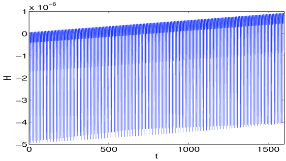
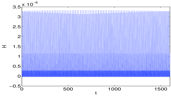
Figure 2.1: Fourth-order Lobatto IIIA method, $h=0.16$, problem (2.1): drift in the Hamiltonian.

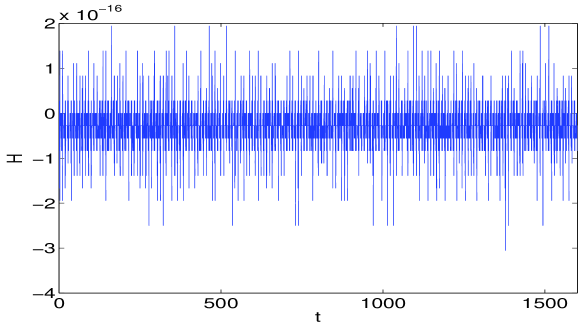
Figure 2.2: Fourth-order Gauss-Legendre method, $h=0.16$, problem (2.1): $H\approx 10^{-6}$.

Figure 2.3: Fourth-order HBVM(6,2) method, $h=0.16$, problem (2.1): $H\approx 10^{-16}$.

Test problem 2

The second test problem, having a highly oscillating solution, is the Fermi-Pasta-Ulam problem (see [21, Section I.5.1]), modelling a chain of 2$m$ mass points connected with alternating soft nonlinear and stiff linear springs, and fixed at the end points. The variables $q_{1},...,q_{2m}$ stand for the displacements of the mass points, and $p_{i}=\dot{q}_{i}$ for their velocities. The corresponding Hamiltonian, representing the total energy, is

$$H(p,q)=\frac{1}{2}\sum_{i=1}^{m}\left(p_{2i-1}^{2}+p_{2i}^{2}\right)+\frac{\omega^{2}}{4}\sum_{i=1}^{m}\left(q_{2i}-q_{2i-1}\right)^{2}+\sum_{i=0}^{m}\left(q_{2i+1}-q_{2i}\right)^{4},$$ (2.2)

with $q_{0}=q_{2m+1}=0$. In our simulation we have used the following values: $m=3$, $\omega=50$, and starting vector

$$p_{i}=0,\quad q_{i}=(i-1)/10,\qquad i=1,\dots,6.$$

In such a case, the Hamiltonian function is a polynomial of degree 4, so that the fourth-order HBVM(4,2) method, either when using the Lobatto nodes or the Gauss-Legendre nodes, is able to exactly preserve the Hamiltonian, as confirmed by the plot in Figure 2.6, obtained with stepsize $h=0.05$. Conversely, by using the same stepsize, both the fourth-order Lobatto IIIA and Gauss-Legendre methods provide only an approximate conservation of the Hamiltonian, as shown in the plots in Figures 2.6 and 2.6, respectively. The fourth-order convergence of the HBVM(4,2) method is numerically verified by the results listed in Table 2.4.

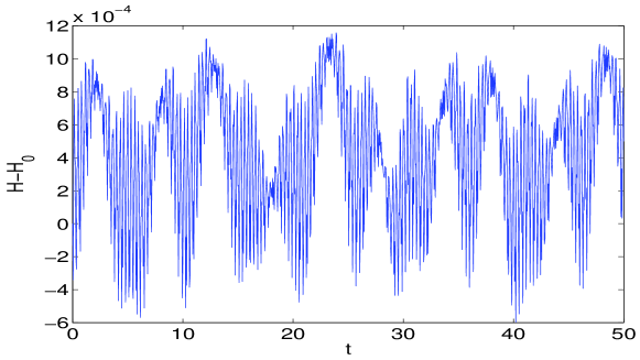
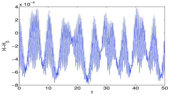
Figure 2.4: Fourth-order Lobatto IIIA method, $h=0.05$, problem (2.2): $|H-H_{0}|\approx 10^{-3}$.

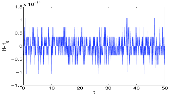
Figure 2.5: Fourth-order Gauss-Legendre method, $h=0.05$, problem (2.2): $|H-H_{0}|\approx 10^{-3}$.

Figure 2.6: Fourth-order HBVM(4,2) method, $h=0.05$, problem (2.2): $|H-H_{0}|\approx 10^{-14}$.

Test problem 3 (non-polynomial Hamiltonian)

In the previous examples, the Hamiltonian function was a polynomial. Nevertheless, as observed above, also in this case HBVM($k$,$s$) are expected to produce a practical conservation of the energy when applied to systems defined by a non-polynomial Hamiltonian function that can be locally well approximated by a polynomial. As an example, we consider the motion of a charged particle in a magnetic field with Biot-Savart potential. It is defined by the Hamiltonian [6]

$$H(x,y,z,\dot{x},\dot{y},\dot{z})=$$

$$\frac{1}{2m}\left[\left(\dot{x}-\alpha\frac{x}{\varrho^{2}}\right)^{2}+\left(\dot{y}-\alpha\frac{y}{\varrho^{2}}\right)^{2}+\left(\dot{z}+\alpha\log(\varrho)\right)^{2}\right],$$

with $\varrho=\sqrt{x^{2}+y^{2}}$, $\alpha=e\,B_{0}$, $m$ is the particle mass, $e$ is its charge, and $B_{0}$ is the magnetic field intensity. We have used the values

$$m=1,\qquad e=-1,\qquad B_{0}=1,$$

with starting point

$$x=0.5,\quad y=10,\quad z=0,\quad\dot{x}=-0.1,\quad\dot{y}=-0.3,\quad\dot{z}=0.$$

By using the fourth-order Lobatto IIIA method, with stepsize $h=0.1$, a drift is again experienced in the numerical solution, as is shown in Figure 2.9. By using the fourth-order Gauss-Legendre method with the same stepsize, the drift disappears even though, as shown in Figure 2.9, the value of the Hamiltonian is preserved within an error of the order of $10^{-3}$. On the other hand, when using the HBVM(6,2) method with the same stepsize, the error in the Hamiltonian decreases to an order of $10^{-15}$ (see Figure 2.9), thus giving a practical conservation. Finally, in Table 2.4 we list the maximum absolute difference between the numerical solutions over $10^{3}$ integration steps, computed by the HBVM$(k,2)$ methods based on Lobatto abscissae and on Gauss-Legendre abscissae, as $k$ grows, with stepsize $h=0.1$. We observe that the difference tends to 0, as $k$ increases. Finally, also in this case, one verifies a fourth-order convergence, as the results listed in Table 2.4 show.

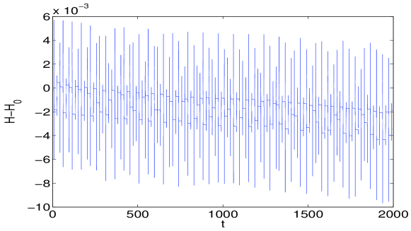
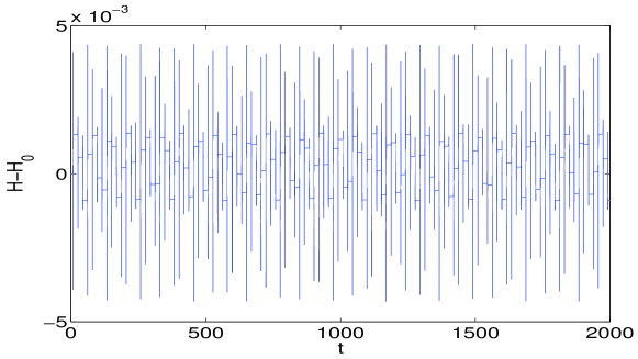
Figure 2.7: Fourth-order Lobatto IIIA method, $h=0.1$, problem (2): drift in the Hamiltonian.

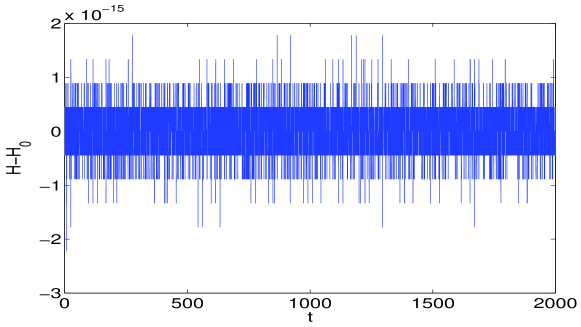
Figure 2.8: Fourth-order Gauss-Legendre method, $h=0.1$, problem (2): $|H-H_{0}|\approx 10^{-3}$.

Figure 2.9: Fourth-order HBVM(6,2) method, $h=0.1$, problem (2): $|H-H_{0}|\approx 10^{-15}$.

Table 2.1: Numerical order of convergence for the HBVM(6,2) method, problem (2.1).

$h$	0.32	0.16	0.08	0.04	0.02
error	$2.288\cdot 10^{-2}$	$1.487\cdot 10^{-3}$	$9.398\cdot 10^{-5}$	$5.890\cdot 10^{-6}$	$3.684\cdot 10^{-7}$
order	–	3.94	3.98	4.00	4.00

Table 2.2: Numerical order of convergence for the HBVM(4,2) method, problem (2.2).

$h$	$1.6\cdot 10^{-2}$	$8\cdot 10^{-3}$	$4\cdot 10^{-3}$	$2\cdot 10^{-3}$	$10^{-3}$
error	$3.030$	$1.967\cdot 10^{-1}$	$1.240\cdot 10^{-2}$	$7.761\cdot 10^{-4}$	$4.853\cdot 10^{-5}$
order	–	3.97	3.99	4.00	4.00

Table 2.3: Numerical order of convergence for the HBVM(6,2) method, problem (2).

$h$	$3.2\cdot 10^{-2}$	$1.6\cdot 10^{-2}$	$8\cdot 10^{-3}$	$4\cdot 10^{-3}$	$2\cdot 10^{-3}$
error	$3.944\cdot 10^{-6}$	$2.635\cdot 10^{-7}$	$1.729\cdot 10^{-8}$	$1.094\cdot 10^{-9}$	$6.838\cdot 10^{-11}$
order	–	3.90	3.93	3.98	4.00

Table 2.4: Maximum difference between the numerical solutions obtained through the fourth-order HBVM$(k,2)$ methods based on Lobatto abscissae and Gauss-Legendre abscissae for increasing values of $k$, problem (2), $10^{3}$ steps with stepsize $h=0.1$.

$k$ $h=0.1$ 2 $3.97\cdot 10^{-1}$ 4 $2.29\cdot 10^{-3}$ 6 $2.01\cdot 10^{-8}$ 8 $1.37\cdot 10^{-11}$ 10 $5.88\cdot 10^{-13}$

Test problem 4 (Sitnikov problem)

The main problem in Celestial Mechanics is the so called $N$-body problem, i.e. to describe the motion of $N$ point particles of positive mass moving under Newton’s law of gravitation when we know their positions and velocities at a given time. This problem is described by the Hamiltonian function:

$$H(\boldsymbol{q},\boldsymbol{p})=\frac{1}{2}\sum_{i=1}^{N}\frac{||p_{i}||_{2}^{2}}{m_{i}}-G\sum_{i=1}^{N}m_{i}\sum_{j=1}^{i-1}\frac{m_{j}}{||q_{i}-q_{j}||_{2}},$$ (2.4)

where $q_{i}$ is the position of the $i$th particle, with mass $m_{i}$, and $p_{i}$ is its momentum.

The Sitnikov problem is a particular configuration of the $3$-body dynamics (see, e.g., [31]). In this problem two bodies of equal mass (primaries) revolve about their center of mass, here assumed at the origin, in elliptic orbits in the $xy$-plane. A third, and much smaller body (planetoid), is placed on the $z$-axis with initial velocity parallel to this axis as well.

The third body is small enough that the two body dynamics of the primaries is not destroyed. Then, the motion of the third body will be restricted to the $z$-axis and oscillating around the origin but not necessarily periodic. In fact this problem has been shown to exhibit a chaotic behavior when the eccentricity of the orbits of the primaries exceeds a critical value that, for the data set we have used, is $\bar{e}\simeq 0.725$ (see Figure 2.10).

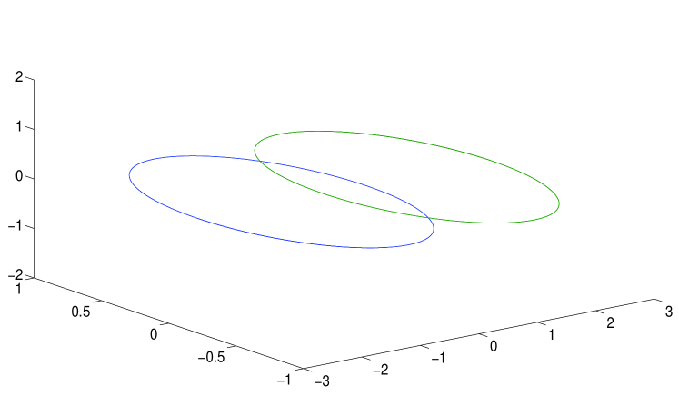
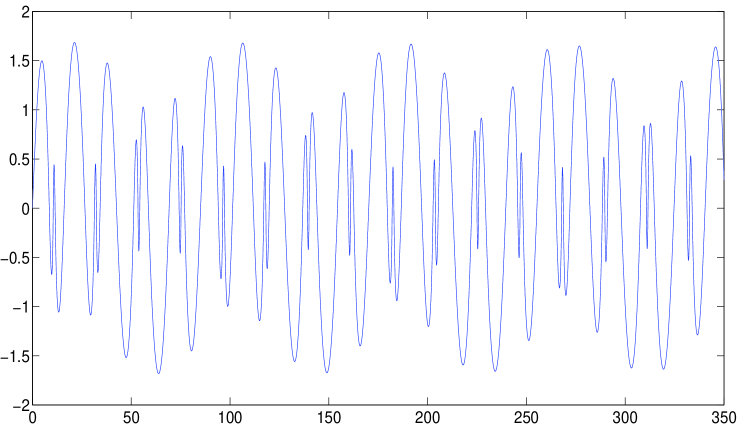
Figure 2.10: The upper picture displays the configuration of $3$-bodies in the Sitnikov problem. To an eccentricity of the orbits of the primaries $e=0.75$, there correspond bounded chaotic oscillations of the planetoid as is argued by looking at the space-time diagram in the down picture.

We have solved the problem defined by the Hamiltonian function (2.4) by the Gauss method of order 4 (i.e., HBVM(2,2) at 2 Gaussian nodes) and by HBVM(18,2) at 18 Gaussian nodes (order 4, $2$ fundamental and $16$ silent stages), with the following set of parameters in (2.4):

$N$	$G$	$m_{1}$	$m_{2}$	$m_{3}$	$e$	$d$	$h$	$t_{\mbox{max}}$
$3$	$1$	$1$	$1$	$10^{-5}$	$0.75$	$5$	$0.5$	$1500$

where $e$ is the eccentricity, $d$ is the distance of the apocentres of the primaries (points at which the two bodies are the furthest), $h$ is the used time-step, and $[0,\,t_{\mbox{max}}]$ is the time integration interval. The eccentricity $e$ and the distance $d$ may be used to define the initial condition $[\boldsymbol{q}_{0},\boldsymbol{p}_{0}]$ (see [31] for the details):

$$\begin{array}[]{l}\boldsymbol{q}_{0}=[-\frac{5}{2},~{}0,~{}0,~{}\frac{5}{2},~{}0,~{}0,~{}0,~{}0,~{}10^{-9}]^{T},\\[2.84544pt] \boldsymbol{p}_{0}=[0,~{}-\frac{1}{20}\sqrt{10},~{}0,~{}0,~{}\frac{1}{20}\sqrt{10},~{}0,~{}0,~{}0,~{}\frac{1}{2}]^{T}.\end{array}$$

First of all, we consider the two pictures in Figure 2.11 reporting the relative errors in the Hamiltonian function and in the angular momentum evaluated along the numerical solutions computed by the two methods. We know that the HBVM(18,2) precisely conserves Hamiltonian polynomial functions of degree at most $18$. This accuracy is high enough to guarantee that the nonlinear Hamiltonian function (2.4) is as well conserved up to the machine precision (see the upper picture): from a geometrical point of view this means that a local approximation of the level curves of (2.4) by a polynomial of degree $18$ leads to a negligible error. The Gauss method exhibits a certain error in the Hamiltonian function while, being this formula symplectic, it precisely conserves the angular momentum, as is confirmed by looking at the down picture of Figure 2.11. The error in the numerical angular momentum associated with the HBVM(18,2) undergoes some bounded periodic-like oscillations.

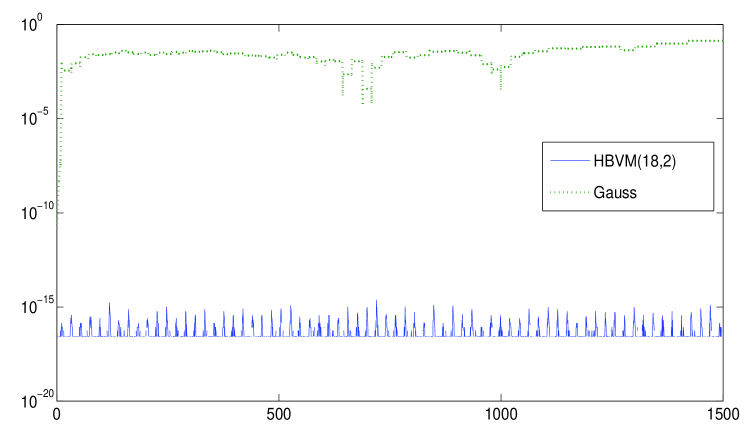
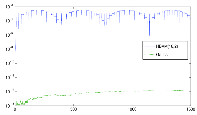
Figure 2.11: Upper picture: relative error $|H(y_{n})-H(y_{0})|/|H(y_{0})|$ of the Hamiltonian function evaluated along the numerical solution of the HBVM($18$,$2$) and the Gauss method. Down picture: relative error $|M(y_{n})-M(y_{0})|/|M(y_{0})|$ of the angular momentum evaluated along the numerical solution of the HBVM($18$,$2$) and the Gauss method.

Figures 2.12 and 2.13 show the numerical solution computed by the Gauss method and HBVM(18,2), respectively. Since the methods leave the $xy$-plane invariant for the motion of the primaries and the $z$-axis invariant for the motion of the planetoid, we have just reported the motion of the primaries in the $xy$-phase plane (upper pictures) and the space-time diagram of the planetoid (down picture).

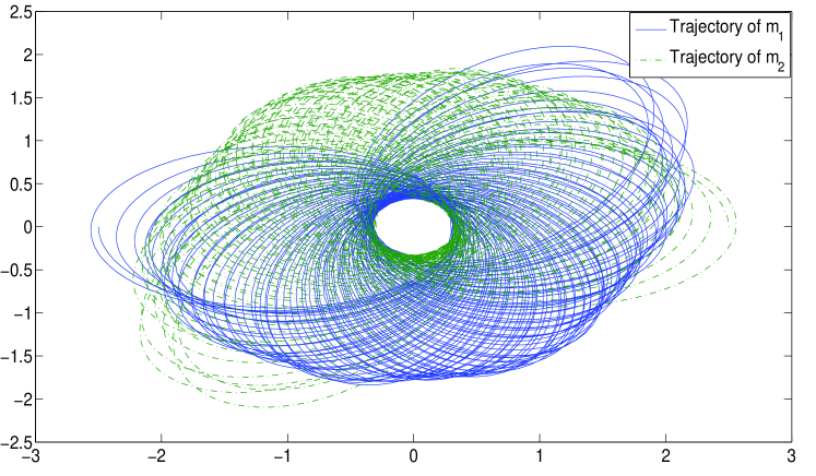
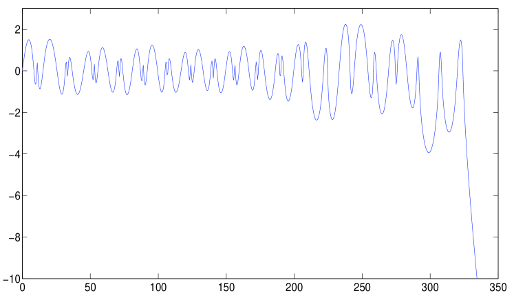
Figure 2.12: The Sitnikov problem solved by the Gauss method of order 4, with stepsize $h=0.5$, in the time interval $[0,1500]$. The trajectories of the primaries in the $xy$-plane (upper picture) exhibit a very irregular behavior which causes the planetoid to eventually escape the system, as illustrated by the space-time diagram in the down picture.

We observe that, for the Gauss method, the orbits of the primaries are irregular in character so that the third body, after performing some oscillations around the origin, will eventually escape the system (see the down picture of Figure 2.12). On the contrary (see the upper picture of Figure 2.13), the HBVM(18,2) method generates a quite regular phase portrait. Due to the large stepsize $h$ used, a sham rotation of the $xy$-plane appears which, however, does not destroy the global symmetry of the dynamics, as testified by the bounded oscillations of the planetoid (down picture of Figure 2.13) which look very similar to the reference ones in Figure 2.10. This aspect is also confirmed by the pictures in Figure 2.14 displaying the distance of the primaries as a function of the time. We see that the distance of the apocentres (corresponding to the maxima in the plots), as the two bodies wheel around the origin, are preserved by the HBVM(18,2) (down picture) while the same is not true for the Gauss method (upper picture).

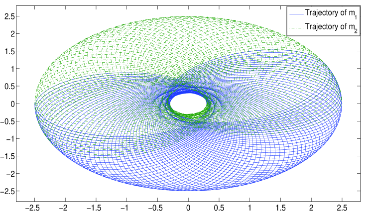
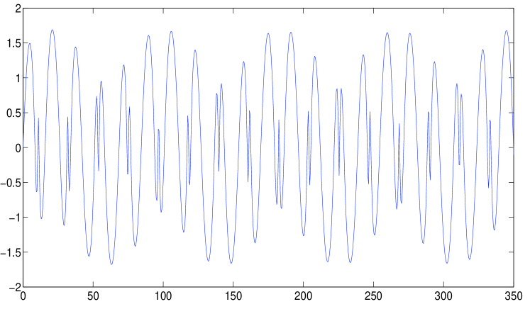
Figure 2.13: The Sitnikov problem solved by the HBVM(18,2) method (order 4), with stepsize $h=0.5$, in the time interval $[0,1500]$. Upper picture: the trajectories of the primaries are ellipse shape. The discretization introduces a fictitious uniform rotation of the $xy$-plane which however does not alter the global symmetry of the system. Down picture: the space-time diagram of the planetoid on the $z$-axis displayed (for clearness) on the time interval $[0,350]$ shows that, although a large value of the stepsize $h$ has been used, the overall behavior of the dynamics is well reproduced (compare with the down picture in Figure 2.10).

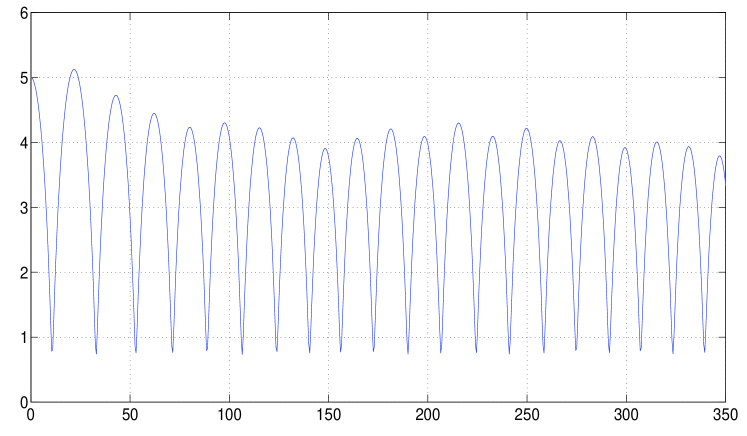
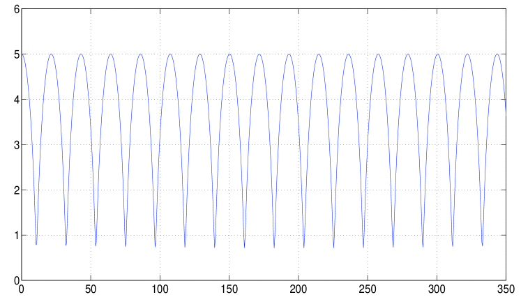
Figure 2.14: Distance between the two primaries as a function of the time, related to the numerical solutions generated by the Gauss method (upper picture) and HBVM(18,2) (down picture). The maxima correspond to the distance of apocentres. These are conserved by HBVM(18,2) while the Gauss method introduces patchy oscillations that destroy the overall symmetry of the system.

Chapter 3 Infinity HBVMs

From the previous arguments, it is clear that the orthogonality conditions (1.13), i.e., the fulfillment of the Master Functional Equation (1.15), is in principle only a sufficient condition for the conservation property (1.12) to hold, when a generic polynomial basis $\{P_{j}\}$ is considered. Such a condition becomes also necessary, when such basis is orthonormal.

Theorem 3.

Let $\{P_{j}\}$ be an orthonormal basis on the interval $[0,1]$. Then, assuming $H(y)$ to be analytical, (1.12) implies that each term in the sum has to vanish.

Proof  Let us consider the expansion

$$g(\tau)\equiv\nabla H(\sigma(t_{0}+\tau h))=\sum_{\ell\geq 1}\rho_{\ell}P_{\ell}(\tau),\qquad\rho_{\ell}=(P_{\ell},g),\qquad\ell\geq 1,$$

where, in general,

$$(f,g)=\int_{0}^{1}f(\tau)g(\tau)\mathrm{d}\tau.$$

Substituting into (1.12), yields

$$\sum_{j=1}^{s}\gamma_{j}^{T}(P_{j},g)=\sum_{j=1}^{s}\gamma_{j}^{T}\left(P_{j},\sum_{\ell\geq 1}\rho_{\ell}P_{\ell}\right)=\sum_{j=1}^{s}\gamma_{j}^{T}\rho_{j}=0.$$

Since this has to hold whatever the choice of the function $H(y)$, one concludes that

$$\gamma_{j}^{T}\rho_{j}=0,\qquad j=1,\dots,s.~{}\mbox{$\Box$}$$ (3.1)

Remark 8.

In the case where $\{P_{j}\}$ is an orthonormal basis, from (3.1) one then derives that

$$\gamma_{j}=S\rho_{j},\qquad i=1,\dots,s,$$

where $S$ is any nonsingular skew-symmetric matrix. The natural choice $S=J$ then leads to (1.13).

Moreover, we observe that, if the Hamiltonian $H(y)$ is a polynomial, the integral appearing at the right-hand side in (1.18) is exactly computed by a quadrature formula, thus resulting into a HBVM($k$,$s$) method with a sufficient number of silent stages. As already stressed in the Chapter 1, in the non-polynomial case such formulae represent the limit of the sequence HBVM($k$,$s$), as $k\rightarrow\infty$.

Definition 3.

For general Hamiltonians, we call the limit formula (1.18) Infinity Hamiltonian Boundary Value Method of degree $s$ (in short, $\infty$-HBVM of degree $s$ or HBVM$(\infty,s)$)  [7].

More precisely, due to the choice of the orthonormal basis (1.8),

$$\mbox{HBVM}(\infty,s)=\lim_{k\rightarrow\infty}\mbox{HBVM}(k,s),$$

whatever is the choice of the fundamental abscissae $\{c_{i}\}$.

A worthwhile consequence of Theorems 1 and 2 is that one can transfer to HBVM$(\infty,s)$ all those properties of HBVM($k$,$s$) which are satisfied starting from a given $k\geq k_{0}$ on: for example, the order and stability properties.

Corollary 1.

Whatever the choice of the abscissae $c_{1},\dots,c_{s}$, HBVM$(\infty,s)$ (1.18) has order $2s$ and is perfectly $A$-stable.

Chapter 4 Isospectral Property of HBVMs and their connections with Runge-Kutta collocation methods

When applied to initial value problems, HBVMs may be viewed as a special subclass of Runge-Kutta (RK) methods of collocation type. In Chapter 1 (see also [6, 7]) the RK formulation turned out useful in stating results pertaining to the order of the new formulae. Here, the RK notation will be exploited to derive the isospectral property of HBVMs and elucidate the existing connections between HBVMs and RK collocation methods [9]. In doing this, our aim is twofold:

1. to better elucidate the close link between the new formulae and the classical collocation Runge-Kutta methods;

2. to make the handling of the new formulae more comfortable to the scientific community working in the context of RK methods.

In fact, we think that HBVMs (and consequently their RK formulation) may be of interest beyond their application to Hamiltonian systems. Each HBVM($k$,$s$) becomes a classical collocation method when $k=s$, while, for $k>s$, it conserves all the features of the generating collocation formula, including the order (which may be even improved, reaching eventually order $p=2s$) and the dimension of the associated nonlinear system.

Let us then consider the matrix appearing in the Butcher tableau (1.27), corresponding to HBVM$(k,s)$, i.e., the matrix

$$A={\cal I}_{s}{\cal P}_{s}^{T}\Omega\in\mathbb{R}^{k\times k},\qquad k\geq s,$$ (4.1)

whose rank is $s$ (see (1.24)–(1.25)). Consequently it has a $(k-s)$-fold zero eigenvalue. To begin with, we are going to discuss the location of the remaining $s$ eigenvalues of that matrix.

Before that, we state the following preliminary result, whose proof can be found in [23, Theorem 5.6 on page 83].

Lemma 1.

The eigenvalues of the matrix

$$X_{s}=\left(\begin{array}[]{cccc}\frac{1}{2}&-\xi_{1}&&\\ \xi_{1}&0&\ddots&\\ &\ddots&\ddots&-\xi_{s-1}\\ &&\xi_{s-1}&0\\ \end{array}\right),$$ (4.2)

with

$$\xi_{j}=\frac{1}{2\sqrt{(2j+1)(2j-1)}},\qquad j=1,\dots,s-1,$$ (4.3)

coincide with those of the matrix in the Butcher tableau of the Gauss-Legendre method of order $2s$.

We also need the following preliminary result, whose proof derives from the properties of shifted-Legendre polynomials (see, e.g., [1] or the Appendix in [6]).

Lemma 2.

With reference to the matrices in (1.24)–(1.25), one has

$${\cal I}_{s}={\cal P}_{s+1}\hat{X}_{s},$$ (4.4)

where

$$\hat{X}_{s}=\left(\begin{array}[]{cccc}\frac{1}{2}&-\xi_{1}&&\\ \xi_{1}&0&\ddots&\\ &\ddots&\ddots&-\xi_{s-1}\\ &&\xi_{s-1}&0\\ \hline\cr&&&\xi_{s}\end{array}\right),$$ (4.5)

with the $\xi_{j}$ defined by (4.3).

The following result then holds true [8].

Theorem 4 (Isospectral Property of HBVMs).

For all $k\geq s$ and for any choice of the abscissae $\{\tau_{i}\}$ such that $B(2s)$ holds true, the nonzero eigenvalues of the matrix $A$ in (4.1) coincide with those of the matrix of the Gauss-Legendre method of order $2s$.

Proof  For $k=s$, the abscissae $\{\tau_{i}\}$ have to be the $s$ Gauss-Legendre nodes on $[0,1]$, so that HBVM$(s,s)$ reduces to the Gauss Legendre method of order $2s$, as already observed in Example 2.

When $k>s$, from the orthonormality of the basis, see (1.7), and considering that the quadrature with weights $\{\omega_{i}\}$ is exact for polynomials of degree (at least) $2s-1$, one easily obtains that

$${\cal P}_{s}^{T}\Omega{\cal P}_{s+1}=\left(I_{s}~{}\boldsymbol{0}\right),$$

since, for all $i=1,\dots,s$,  and  $j=1,\dots,s+1$:

$$\left({\cal P}_{s}^{T}\Omega{\cal P}_{s+1}\right)_{ij}=\sum_{\ell=1}^{k}\omega_{\ell}P_{i}(\tau_{\ell})P_{j}(\tau_{\ell})=\int_{0}^{1}P_{i}(t)P_{j}(t)\mathrm{d}t=\delta_{ij}.$$

By taking into account the result of Lemma 2, one then obtains:

$$A{\cal P}_{s+1} = {\cal I}_{s}{\cal P}_{s}^{T}\Omega{\cal P}_{s+1}={\cal I}_{s}\left(I_{s}~{}\boldsymbol{0}\right)={\cal P}_{s+1}\hat{X}_{s}\left(I_{s}~{}\boldsymbol{0}\right)={\cal P}_{s+1}\left(\hat{X}_{s}~{}\boldsymbol{0}\right)$$ (4.11)

$$= {\cal P}_{s+1}\left(\begin{array}[]{cccc|c}\frac{1}{2}&-\xi_{1}&&&0\\ \xi_{1}&0&\ddots&&\vdots\\ &\ddots&\ddots&-\xi_{s-1}&\vdots\\ &&\xi_{s-1}&0&0\\ \hline\cr&&&\xi_{s}&0\end{array}\right)\equiv{\cal P}_{s+1}\widetilde{X}_{s},$$

with the $\{\xi_{j}\}$ defined according to (4.3). Consequently, one obtains that the columns of ${\cal P}_{s+1}$ constitute a basis of an invariant (right) subspace of matrix $A$, so that the eigenvalues of $\widetilde{X}_{s}$ are eigenvalues of $A$. In more detail, the eigenvalues of $\widetilde{X}_{s}$ are those of $X_{s}$ (see (4.2)) and the zero eigenvalue. Then, also in this case, the nonzero eigenvalues of $A$ coincide with those of $X_{s}$, i.e., with the eigenvalues of the matrix defining the Gauss-Legendre method of order $2s$. $\Box$

4.1 HBVMs and collocation methods

By using the previous result and notations, now we go to elucidate the existing connections between HBVMs and RK collocation methods. We shall continue to use an orthonormal basis $\{P_{j}\}$, along which the underlying extended collocation polynomial $\sigma(t)$ is expanded, even though the arguments could be generalized to more general bases, as sketched below. On the other hand, the distribution of the internal abscissae can be arbitrary.

Our starting point is a generic collocation method with $k$ stages, defined by the tableau

$$\begin{array}[]{c|c}\begin{array}[]{c}\tau_{1}\\ \vdots\\ \tau_{k}\end{array}&\mathcal{A}\\ \hline\cr&\omega_{1}\,\ldots~{}\omega_{k}\end{array}$$ (4.12)

where, for $i,j=1,\dots,k$, $\mathcal{A}=\left(\alpha_{ij}\right)\equiv\left(\int_{0}^{\tau_{i}}\ell_{j}(\tau)\mathrm{d}\tau\right)$ and $\omega_{j}=\int_{0}^{1}\ell_{j}(\tau)\mathrm{d}\tau$, $\ell_{j}(t)$ being the $j$th Lagrange polynomial of degree $k-1$ defined on the set of abscissae $\{\tau_{i}\}$.

Given a positive integer $s\leq k$, we can consider a basis $\{p_{1}(\tau),\dots,p_{s}(\tau)\}$ of the vector space of polynomials of degree at most $s-1$, and we set

$$\hat{\cal P}_{s}=\left(\begin{array}[]{cccc}p_{1}(\tau_{1})&p_{2}(\tau_{1})&\cdots&p_{s}(\tau_{1})\\ p_{1}(\tau_{2})&p_{2}(\tau_{2})&\cdots&p_{s}(\tau_{2})\\ \vdots&\vdots&&\vdots\\ p_{1}(\tau_{k})&p_{2}(\tau_{k})&\cdots&p_{s}(\tau_{k})\end{array}\right)_{k\times s}$$ (4.13)

(note that $\hat{\cal P}_{s}$ is full rank since the nodes are distinct). The class of RK methods we are interested in is defined by the tableau

$$\begin{array}[]{c|c}\begin{array}[]{c}\tau_{1}\\ \vdots\\ \tau_{k}\end{array}&A\equiv\mathcal{A}\hat{\cal P}_{s}\Lambda_{s}\hat{\cal P}_{s}^{T}\Omega\\ \hline\cr&\omega_{1}\,\ldots\ldots~{}\omega_{k}\end{array}$$ (4.14)

where $\Omega={\rm diag}(\omega_{1},\dots,\omega_{k})$ and $\Lambda_{s}={\rm diag}(\eta_{1},\dots,\eta_{s})$; the coefficients $\eta_{j}$, $j=1,\dots,s$, have to be selected by imposing suitable consistency conditions on the stages $\{Y_{i}\}$ [7]. In particular, when the basis is orthonormal, as we shall assume hereafter, then matrix $\hat{\cal P}_{s}$ reduces to matrix ${\cal P}_{s}$ in (1.24)–(1.25), $\Lambda_{s}=I_{s}$, and consequently (4.14) becomes

$$\begin{array}[]{c|c}\begin{array}[]{c}\tau_{1}\\ \vdots\\ \tau_{k}\end{array}&A\equiv\mathcal{A}{\cal P}_{s}{\cal P}_{s}^{T}\Omega\\ \hline\cr&\omega_{1}\,\ldots\ldots~{}\omega_{k}\end{array}$$ (4.15)

We note that the Butcher array $A$ has rank which cannot exceed $s$, because it is defined by filtering $\mathcal{A}$ by the rank $s$ matrix ${\cal P}_{s}{\cal P}_{s}^{T}\Omega$.

The following result then holds true, which clarifies the existing connections between classical RK collocation methods and HBVMs.

Theorem 5.

Provided that the quadrature formula defined by the weights $\{\omega_{i}\}$ is exact for polynomials at least $2s-1$ (i.e., the RK method defined by the tableau (4.15) satisfies the usual simplifying assumption $B(2s)$), then the tableau (4.15) defines a HBVM$(k,s)$ method based at the abscissae $\{\tau_{i}\}$.

Proof Let us expand the basis $\{P_{1}(\tau),\dots,P_{s}(\tau)\}$ along the Lagrange basis $\{\ell_{j}(\tau)\}$, $j=1,\dots,k$, defined over the nodes $\tau_{i}$, $i=1,\dots,k$:

$$P_{j}(\tau)=\sum_{r=1}^{k}P_{j}(\tau_{r})\ell_{r}(\tau),\qquad j=1,\dots,s.$$

It follows that, for $i=1,\dots,k$ and $j=1,\dots,s$:

$$\int_{0}^{\tau_{i}}P_{j}(x)\mathrm{d}x=\sum_{r=1}^{k}P_{j}(\tau_{r})\int_{0}^{\tau_{i}}\ell_{r}(x)\mathrm{d}x=\sum_{r=1}^{k}P_{j}(\tau_{r})\alpha_{ir},$$

that is (see (1.24)–(1.25) and (4.12)),

$${\cal I}_{s}=\mathcal{A}{\cal P}_{s}.$$ (4.16)

By substituting (4.16) into (4.15), one retrieves that tableau (1.27), which defines the method HBVM$(k,s)$. This completes the proof. $\Box$

The resulting Runge-Kutta method (4.15) is then energy conserving if applied to polynomial Hamiltonian systems (1.1) when the degree of $H(y)$, is lower than or equal to a quantity, say $\nu$, depending on $k$ and $s$. As an example, when a Gaussian distribution of the nodes $\{\tau_{i}\}$ is considered, one obtains (1.29).

Remark 9 (About Simplecticity).

The choice of the abscissae $\{\tau_{1},\dots,\tau_{k}\}$ at the Gaussian points in $[0,1]$ has also another important consequence, since, in such a case, the collocation method (4.12) is the Gauss method of order $2k$ which, as is well known, is a symplectic method. The result of Theorem 5 then states that, for any $s\leq k$, the HBVM$(k,s)$ method is related to the Gauss method of order $2k$ by the relation:

$$A={\cal A}({\cal P}_{s}{\cal P}_{s}^{T}\Omega),$$

where the filtering matrix $({\cal P}_{s}{\cal P}_{s}^{T}\Omega)$ essentially makes the Gauss method of order $2k$ “work” in a suitable subspace.

It seems like the price paid to achieve such conservation properties consists in the lowering of the order of the new method with respect to the original one (4.12). Actually this is not true, because a fair comparison would be to relate method (1.27)–(4.15) to a collocation method constructed on $s$ rather than on $k$ stages. This fact will be fully elucidated in Chapter 5.

4.1.1 An alternative proof for the order of HBVMs

We conclude this chapter by observing that the order $2s$ of an HBVM$(k,s)$ method, under the hypothesis that (4.12) satisfies the usual simplifying assumption $B(2s)$, i.e., the quadrature defined by the weights $\{\omega_{i}\}$ is exact for polynomials of degree at least $2s-1$, may be stated by using an alternative, though equivalent, procedure to that used in the proof of Theorem 1.

Let us then define the $k\times k$ matrix ${\cal P}\equiv{\cal P}_{k}$ (see (1.24)–(1.25)) obtained by “enlarging” the matrix ${\cal P}_{s}$ with $k-s$ columns defined by the normalized shifted Legendre polynomials $P_{j}(\tau)$, $j=s+1,\dots,k$, evaluated at $\{\tau_{i}\}$, i.e.,

$${\cal P}=\left(\begin{array}[]{ccc}P_{1}(\tau_{1})&\dots&P_{k}(\tau_{1})\\ \vdots&&\vdots\\ P_{1}(\tau_{k})&\dots&P_{k}(\tau_{k})\end{array}\right).$$

By virtue of property $B(2s)$ for the quadrature formula defined by the weights $\{\omega_{i}\}$, it satisfies

$${\cal P}^{T}\Omega{\cal P}=\left(\begin{array}[]{ll}I_{s}&O\\ O&R\end{array}\right),\qquad R\in\mathbb{R}^{k-s\times k-s}.$$

This implies that ${\cal P}$ satisfies the property $T(s,s)$ in [23, Definition 5.10 on page 86], for the quadrature formula $(\omega_{i},\tau_{i})_{i=1}^{k}$. Therefore, for the matrix $A$ appearing in (4.15) (i.e., (1.27), by virtue of Theorem 5), one obtains:

$${\cal P}^{-1}A{\cal P}={\cal P}^{-1}\mathcal{A}{\cal P}\left(\begin{array}[]{ll}I_{s}\\ &O\end{array}\right)=\left(\begin{array}[]{ll}\widetilde{X}_{s}\\ &O\end{array}\right),$$ (4.17)

where $\widetilde{X}_{s}$ is the matrix defined in (4.11). Relation (4.17) and [23, Theorem 5.11 on page 86] prove that method (4.15) (i.e., HBVM$(k,s)$) satisfies $C(s)$ and $D(s-1)$ and, hence, its order is $2s$.

Remark 10 (Invariance of the order).

From the previous result we deduce the invariance of the superconvergence property of HBVM($k$,$s$) with respect to the distribution of the abscissae $\tau_{i}$, $i=1,\dots,k$, the only assumption to get the order $2s$ being that the underlying quadrature formula has degree of precision $2s-1$. Such exceptional circumstance is likely to have interesting applications beyond the purposes here presented.

Chapter 5 Blended HBVMs

We shall now consider some computational aspects concerning HBVM$(k,s)$. In more details, we now show how its cost depends essentially on $s$, rather than on $k$, in the sense that the nonlinear system to be solved, for obtaining the discrete solution, has (block) dimension $s$ [3, 6, 8].

This could be inferred from the fact that the silent stages (1.11) depend on the fundamental stages: let us see the details. In order to simplify the notation, we shall fix the fundamental stages at $\tau_{1},\dots,\tau_{s}$, since we have already seen that, due to the use of an orthonormal basis, they could be in principle chosen arbitrarily, among the abscissae $\{\tau_{i}\}$. With this premise, we have, from (1), (1.17)–(1.18), and by using the notation (LABEL:tiyi),

$$y_{i}=y_{0}+h\sum_{j=1}^{s}a_{ij}\sum_{\ell=1}^{k}\omega_{\ell}P_{j}(\tau_{\ell})f_{\ell},\qquad i=1,\dots,s.$$ (5.1)

This equation is now coupled with that defining the silent stages, i.e., from (1.6) and (1.11),

$$y_{i}=y_{0}+h\sum_{j=1}^{s}\gamma_{j}\int_{0}^{\tau_{i}}P_{j}(t)\mathrm{d}t,\qquad i=s+1,\dots,k.$$ (5.2)

Let us now partition the matrices ${\cal I}_{s},{\cal P}_{s}\in\mathbb{R}^{k\times s}$ in (1.24)–(1.25) into

$${\cal I}_{s1},{\cal P}_{s1}\in\mathbb{R}^{s\times s},\qquad{\cal I}_{s2},{\cal P}_{s2}\in\mathbb{R}^{k-s\times s},$$

containing the entries defined by the fundamental abscissae and the silent abscissae, respectively. Similarly, we partition the vector $\boldsymbol{y}$ into $\boldsymbol{y}_{1}$, containing the fundamental stages, and $\boldsymbol{y}_{2}$ containing the silent stages and, accordingly, let

$$\Omega_{1}\in\mathbb{R}^{s\times s},\qquad\Omega_{2}\in\mathbb{R}^{k-s\times k-s},$$

be the diagonal matrices containing the corresponding entries in matrix $\Omega$. Finally, let us define the vectors

$$\boldsymbol{\gamma}=(\gamma_{1},\dots,\gamma_{s})^{T},\qquad e=(1,\dots,1)^{T}\in\mathbb{R}^{s},\qquad u=(1,\dots,1)^{T}\in\mathbb{R}^{k-s}.$$

Consequently, we can rewrite (5.1) and (5.2), as

$$\boldsymbol{y}_{1} = e\otimes y_{0}+h{\cal I}_{s1}\left({\cal P}_{s1}^{T}~{}{\cal P}_{s2}^{T}\right)\left(\begin{array}[]{cc}\Omega_{1}\\ &\Omega_{2}\end{array}\right)\otimes I_{2m}\left(\begin{array}[]{c}f(\boldsymbol{y}_{1})\\ f(\boldsymbol{y}_{2})\end{array}\right),$$ (5.7)

$$\boldsymbol{y}_{2} = u\otimes y_{0}+h{\cal I}_{s2}\otimes I_{2m}\boldsymbol{\gamma},$$ (5.8)

respectively. The vector $\boldsymbol{\gamma}$ can be obtained by the identity (see (1.16))

$$\boldsymbol{y}_{1}=e\otimes y_{0}+h{\cal I}_{s1}\otimes I_{2m}\boldsymbol{\gamma},$$

thus giving

$$\boldsymbol{y}_{2} = \left(u-{\cal I}_{s2}{\cal I}_{s1}^{-1}e\right)\otimes y_{0}+{\cal I}_{s2}{\cal I}_{s1}^{-1}\otimes I_{2m}\boldsymbol{y}_{1}$$ (5.9)

$$\equiv \hat{u}\otimes y_{0}+A_{1}\otimes I_{2m}\boldsymbol{y}_{1},$$

in place of (5.8), where, evidently,

$$\hat{u}=\left(u-{\cal I}_{s2}{\cal I}_{s1}^{-1}e\right)\in\mathbb{R}^{k-s},\qquad A_{1}={\cal I}_{s2}{\cal I}_{s1}^{-1}\in\mathbb{R}^{k-s\times s}.$$ (5.10)

By setting

$$B_{1}={\cal I}_{s1}{\cal P}_{s1}^{T}\Omega_{1}\in\mathbb{R}^{s\times s},\qquad B_{2}={\cal I}_{s1}{\cal P}_{s2}^{T}\Omega_{2}\in\mathbb{R}^{s\times k-s},$$ (5.11)

substitution of (5.9) into (5.7) then provides, at last, the system of block size $s$ to be actually solved:

$$F(\boldsymbol{y}_{1}) \equiv \boldsymbol{y}_{1}-e\otimes y_{0}-h\left[B_{1}\otimes I_{2m}f(\boldsymbol{y}_{1})+\right.$$

$$\left.B_{2}\otimes I_{2m}f\left(\hat{u}\otimes y_{0}+A_{1}\otimes I_{2m}\boldsymbol{y}_{1}\right)\right]=\bf 0.$$

By using the simplified Newton method for solving (5), and setting

$$C=B_{1}+B_{2}A_{1}\in\mathbb{R}^{s\times s},$$ (5.13)

one obtains the iteration:

$$\left(I_{s}\otimes I_{2m}-hC\otimes J_{0}\right)\boldsymbol{\delta}^{(n)} = -F(\boldsymbol{y}_{1}^{(n)})\equiv\boldsymbol{\psi}_{1}^{(n)},$$ (5.14)

$$\boldsymbol{y}_{1}^{(n+1)} = \boldsymbol{y}_{1}^{(n)}+\boldsymbol{\delta}^{(n)},\qquad n=0,1,\dots,$$

where $J_{0}$ is the Jacobian of $f(y)$ evaluated at $y_{0}$. Because of the result of Theorem 4, the following property of matrix $C$ holds true  [8].

Theorem 6.

The eigenvalues of matrix $C$ in (5.13) coincide with those of matrix (4.2), i.e., with the eigenvalues of the matrix of the Butcher array of the Gauss-Legendre method of order $2s$.

Proof Assuming, as usual for simplicity, that the fundamental stages are the first $s$ ones, one has that the discrete problem

$$\boldsymbol{y}=\left(\begin{array}[]{c}e\\ u\end{array}\right)\otimes y_{0}+hA\otimes I_{2m}f(\boldsymbol{y}),$$

which defines the Runge-Kutta formulation of the method, is equivalent, by virtue of (5.7), (5.9), (5.10), (5.11), to

$$\left(\begin{array}[]{cc}I_{s}&O_{s\times r}\\ -A_{1}&I_{r}\end{array}\right)\otimes I_{2m}\left(\begin{array}[]{c}\boldsymbol{y}_{1}\\ \boldsymbol{y}_{2}\end{array}\right)=$$

$$\left(\begin{array}[]{c}e\\ \hat{u}\end{array}\right)\otimes y_{0}+h\left(\begin{array}[]{cc}B_{1}&B_{2}\\ O_{r\times s}&O_{r\times r}\end{array}\right)\otimes I_{2m}\left(\begin{array}[]{c}f(\boldsymbol{y}_{1})\\ f(\boldsymbol{y}_{2})\end{array}\right),$$

where, as usual, $r=k-s$. Consequently, the eigenvalues of the matrix $A$ defined in (4.1) coincides with those of the pencil

$$\left(~{}\left(\begin{array}[]{cc}I_{s}&O_{s\times r}\\ -A_{1}&I_{r}\end{array}\right),~{}\left(\begin{array}[]{cc}B_{1}&B_{2}\\ O_{r\times s}&O_{r\times r}\end{array}\right)~{}\right).$$ (5.17)

That is,

$$\mu\in\sigma(A)~{}~{}\Leftrightarrow~{}~{}\mu\left(\begin{array}[]{cc}I_{s}&O_{s\times r}\\ -A_{1}&I_{r}\end{array}\right)\left(\begin{array}[]{c}\boldsymbol{u}\\ \boldsymbol{v}\end{array}\right)=\left(\begin{array}[]{cc}B_{1}&B_{2}\\ O_{r\times s}&O_{r\times r}\end{array}\right)\left(\begin{array}[]{c}\boldsymbol{u}\\ \boldsymbol{v}\end{array}\right),$$

for some nonzero vector $(\boldsymbol{u}^{T},\boldsymbol{v}^{T})^{T}$. By setting $\boldsymbol{u}=\boldsymbol{0}$, one obtains the $r$ zero eigenvalues of the pencil. For the remaining $s$ (nonzero) ones, it must be $\boldsymbol{v}=A_{1}\boldsymbol{u}$, so that:

$$\mu\boldsymbol{u}=\left(B_{1}\boldsymbol{u}+B_{2}\boldsymbol{v}\right)=\left(B_{1}\boldsymbol{u}+B_{2}A_{1}\boldsymbol{u}\right)=C\boldsymbol{u}~{}~{}\Leftrightarrow~{}~{}\mu\in\sigma(C).~{}\mbox{$\Box$}$$

Remark 11.

From the result of Theorem 6, it follows that the spectrum of $C$ doesn’t depend on the choice of the $s$ fundamental abscissae, within the nodes $\{\tau_{i}\}$. On the contrary, its condition number does: the latter appears to be minimized when the fundamental abscissae are symmetrically distributed and approximately evenly spaced in the interval $[0,1]$. As a practical “rule of thumb”, the following algorithm appears to be almost optimal:

1. let the $k$ abscissae $\{\tau_{i}\}$ be chosen according to a Gauss-Legendre distribution of $k$ nodes;

2. then, let us consider $s$ equidistributed nodes in $(0,1)$, say $\{\hat{\tau}_{1},\dots,\hat{\tau}_{s}\}$;

3. select, as the fundamental abscissae, those nodes among the $\{\tau_{i}\}$ which are the closest ones to the $\{\hat{\tau}_{j}\}$;

4. define matrix $C$ in (5.13) accordingly.

Clearly, for the above algorithm to provide a unique solution (resulting in a symmetric choice of the fundamental abscissae), the difference $k-s$ has to be even which, however, can be easily accomplished.

In order to give evidence of the effectiveness of the above algorithm, in Figure 5.2 we plot the condition number of matrix $C=C(k,s)$, for $s=2,\dots,5$, and $k\geq s$. As one can see, the condition number of $C(k,s)$ turns out to be nicely bounded, for increasing values of $k$, which makes the implementation (that we are going to analyze in the next section) effective also when finite precision arithmetic is used. For comparison, in Figure 5.2 there is the same plot, obtained by fixing the fundamental abscissae as the first $s$ ones. In such a case, the condition number of $C(k,s)$ grows very fast, as $k$ is increased.

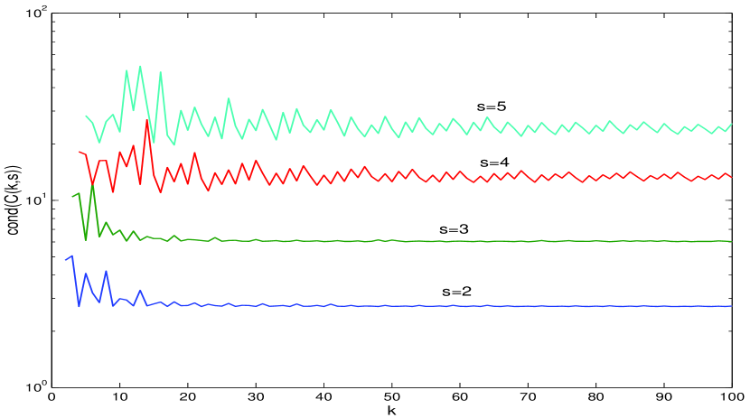
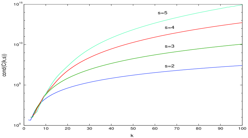
Figure 5.1: Condition number of the matrix $C=C(k,s)$, for $s=2,3,4,5$ and $k=s,s+1,\dots,100$, with the fundamental abscissae chosen according to the algorithm sketched in Remark 11.

Figure 5.2: Condition number of the matrix $C=C(k,s)$, for $s=2,3,4,5$ and $k=s,s+1,\dots,100$, with the fundamental abscissae chosen as the first $s$ ones.

5.1 Blended implementation

We observe that, since $C$ is nonsingular, we can recast problem (5.14) in the equivalent form

$$\gamma\left(C^{-1}\otimes I_{2m}-hI_{s}\otimes J_{0}\right)\boldsymbol{\delta}^{(n)}=-\gamma C^{-1}\otimes I_{2m}\,F(\boldsymbol{y}_{1}^{(n)})\equiv\boldsymbol{\psi}_{2}^{(n)},$$ (5.18)

where $\gamma>0$ is a free parameter to be chosen later. Let us now introduce the weight (matrix) function

$$\theta=I_{s}\otimes\Phi^{-1},\qquad\Phi=I_{2m}-h\gamma J_{0}\in\mathbb{R}^{2m\times 2m},$$ (5.19)

and the blended formulation of the system to be solved,

$$M\boldsymbol{\delta}^{(n)} \equiv \left[\theta\left(I_{s}\otimes I_{2m}-hC\otimes J_{0}\right)+\right.$$ (5.20)

$$\left.(I-\theta)\gamma\left(C^{-1}\otimes I_{2m}-hI_{s}\otimes J_{0}\right)\right]\boldsymbol{\delta}^{(n)}$$

$$= \theta\boldsymbol{\psi}_{1}^{(n)}+(I-\theta)\boldsymbol{\psi}_{2}^{(n)}\equiv\boldsymbol{\psi}^{(n)}.$$

The latter system has again the same solution as the previous ones, since it is obtained as the blending, with weights $\theta$ and $(I-\theta)$, of the two equivalent forms (5.14) and (5.18). For iteratively solving (5.20), we use the corresponding blended iteration, formally given by [2, 10, 11, 12, 13, 14, 15, 16, 18, 30, 32]:

$$\boldsymbol{\delta}^{(n,\ell+1)}=\boldsymbol{\delta}^{(n,\ell)}-\theta\left(M\boldsymbol{\delta}^{(n,\ell)}-\boldsymbol{\psi}^{(n)}\right),\qquad\ell=0,1,\dots.$$ (5.21)

Remark 12.

A nonlinear variant of the iteration (5.21) can be obtained, by starting at $\boldsymbol{\delta}^{(n,0)}=\bf 0$ and updating $\boldsymbol{\psi}^{(n)}$ as soon as a new approximation is available. This results in the following iteration:

$$\boldsymbol{y}^{(n+1)}=\boldsymbol{y}^{(n)}+\theta\boldsymbol{\psi}^{(n)},\qquad n=0,1,\dots.$$ (5.22)

Remark 13.

We observe that, for actually performing the iteration (5.19)–(5.21), as well as (5.22), one has to factor only the matrix $\Phi$ in (5.19), which has the same size as that of the continuous problem.

We end this section by observing that the above iterations (5.21) and (5.22) depend on a free parameter $\gamma$. It will be chosen in order to optimize the convergence properties of the iteration, according to a linear analysis of convergence, which is sketched in the next section.

5.2 Linear analysis of convergence

The linear analysis of convergence for the iteration (5.21) is carried out by considering the usual scalar test equation (see, e.g., [14] and the references therein),

$$y^{\prime}=\lambda y,\qquad\Re(\lambda)<0.$$

By setting, as usual $q=h\lambda$, the two equivalent formulations (5.14) and (5.18) become, respectively (omitting, for sake of brevity, the upper index $n$),

$$(I_{s}-qC)\boldsymbol{\delta}=\boldsymbol{\psi}_{1},\qquad\gamma(C^{-1}-qI_{s})\boldsymbol{\delta}=\boldsymbol{\psi}_{2}.$$

Moreover,

$$\theta=\theta(q)=(1-\gamma q)^{-1}I_{s},$$ (5.23)

and the blended iteration (5.21) becomes

$$\boldsymbol{\delta}^{(\ell+1)}=(I_{s}-\theta(q)M(q))\boldsymbol{\delta}^{(\ell)}+\theta(q)\boldsymbol{\psi}(q),$$ (5.24)

with

$$M(q) = \theta(q)\left(I_{s}-qC\right)+(I_{s}-\theta(q))\gamma\left(C^{-1}-qI_{s}\right),$$ (5.25)

$$\boldsymbol{\psi}(q) = \theta(q)\boldsymbol{\psi}_{1}+(I_{s}-\theta(q))\boldsymbol{\psi}_{2}.$$

Consequently, the iteration will be convergent if and only if the spectral radius $\rho(q)$ of the iteration matrix,

$$Z(q)=I_{s}-\theta(q)M(q),$$ (5.26)

is less than 1. The set

$$\Gamma=\left\{q\in\mathbb{C}\,:\,\rho(q)<1\right\}$$

is the region of convergence of the iteration. The iteration is said to be:

• $A$-convergent,   if $\mathbb{C}^{-}\subseteq\Gamma$;

• $L$-convergent,   if it is $A$-convergent and, moreover,  $\rho(q)\rightarrow 0$,  as  $q\rightarrow\infty$.

Table 5.1: optimal values (5.29), and corresponding maximum amplification factors (5.30), for various values of $s$.

$s$ $\gamma$ $\rho^{*}$ 2 0.2887 0.1340 3 0.1967 0.2765 4 0.1475 0.3793 5 0.1173 0.4544 6 0.0971 0.5114 7 0.0827 0.5561 8 0.0718 0.5921 9 0.0635 0.6218 10 0.0568 0.6467

For the iteration (5.24) one verifies that (see (5.23), (5.25), and (5.26))

$$Z(q)=\frac{q}{(1-\gamma q)^{2}}C^{-1}\left(C-\gamma I_{s}\right)^{2},$$ (5.27)

which is the null matrix at $q=0$ and at $\infty$. Consequently, the iteration will be $A$-convergent (and, therefore, $L$-convergent), provided that maximum amplification factor,

$$\rho^{*}\equiv\max_{\Re(q)=0}\rho(q)~{}\leq 1.$$ (5.28)

From (5.27) one has that, by setting hereafter $\sigma(C)$ the spectrum of matrix $C$,

$$\mu\in\sigma(C)~{}\Leftrightarrow~{}\frac{q(\mu-\gamma)^{2}}{\mu(1-\gamma q)^{2}}\in\sigma(Z(q)).$$

By taking into account that

$$\max_{\Re(q)=0}\frac{|q|}{|(1-\gamma q)^{2}|}=\frac{1}{2\gamma},$$

one then obtains that

$$\rho^{*}=\max_{\mu\in\sigma(C)}\frac{|\mu-\gamma|^{2}}{2\gamma|\mu|},$$

For Gauss-Legendre methods (and, then, for any matrix $C$ having the same spectrum), it can be shown that (see [10, 16]) the choice

$$\gamma=|\mu_{\min}|\equiv\min_{\mu\in\sigma(C)}|\mu|,$$ (5.29)

minimizes $\rho^{*}$, which turns out to be given by

$$\rho^{*}=1-\cos\varphi_{\min}~{}<1,\qquad\varphi_{\min}={\rm Arg}(\mu_{\min}).$$ (5.30)

In Table 5.1, we list the optimal value of the parameter $\gamma$, along with the corresponding maximum amplification factor $\rho^{*}$, for various values of $s$, which confirm that the iteration (5.24) is $L$-convergent.

Remark 14.

We then conclude that the blended iteration (5.21) turns out to be $L$-convergent, for any HBVM$(k,s)$ method, for all $s\geq 1$ and $k\geq s$.

We end this chapter, by emphasizing that the property of $L$-convergence has proved to be computationally very effective, as testified by the successful implementation of the codes BiM and BiMD [30, 32]. We then expect good performances also for the blended implementation of HBVM$(k,s)$.

Chapter 6 Notes and References

The approach of using discrete line integrals has been used, at first, by Iavernaro and Trigiante, in connection with the study of the properties of the trapezoidal rule [26, 27, 28].

It has been then extended by Iavernaro and Pace [24], thus providing the first example of conservative methods, basically an extension of the trapezoidal rule, named $s$-stage trapezoidal methods: this is a family of energy-preserving methods of order 2, able to preserve polynomial Hamiltonian functions of arbitrarily high degree.

Later generalizations allowed Iavernaro and Pace [25], and then Iavernaro and Trigiante [29], to derive energy preserving methods of higher order.

The general approach, involving the shifted Legendre polynomial basis, which has allowed a full complete analysis of HBVMs, has been introduced in [6] (see also [5]) and, subsequently, developed in [7].

The Runge-Kutta formulation of HBVMs, along with their connections with collocation methods, has been studied in [9].

The isospectral property of HBVMs has been also studied in [8], where the blended implementation of the methods has been also introduced.

Computational aspects, concerning both the computational cost and the efficient numerical implementation of HBVMs, have been studied in [3] and [8].

Relevant examples have been collected in [4], where the potentialities of HBVMs are clearly outlined, also demonstrating their effectiveness with respect to standard symmetric and symplectic methods.

Blended implicit methods have been studied in a series of papers [2, 10, 11, 12, 13, 14, 15, 16, 30] and have been implemented in the two computational codes BiM and BiMD [32].

Bibliography

- [1] M. Abramovitz, I.A. Stegun. Handbook of Mathematical Functions. Dover, 1965.
- [2] L. Brugnano. Blended block BVMs (B3VMs): A family of economical implicit methods for ODEs. J. Comput. Appl.Math. 116 (2000) 41–62.
- [3] L. Brugnano, F. Iavernaro, T. Susca. Hamiltonian BVMs (HBVMs): implementation details and applications. “Proceedings of ICNAAM 2009”, AIP Conf. Proc. 1168 (2009) 723–726.
- [4] L. Brugnano, F. Iavernaro, T. Susca. Numerical comparisons between Gauss-Legendre methods and Hamiltonian BVMs defined over Gauss points. Monografías de la Real Academia de Ciencias de Zaragoza, Special Issue devoted to the 65th birthday of Manuel Calvo, (Submitted) 2010 (arXiv:1002.2727).
- [5] L. Brugnano, F. Iavernaro, D. Trigiante. Hamiltonian BVMs (HBVMs): a family of “drift-free” methods for integrating polynomial Hamiltonian systems. “Proceedings of ICNAAM 2009”, AIP Conf. Proc. 1168 (2009) 715–718.
- [6] L. Brugnano, F. Iavernaro, D. Trigiante. Analisys of Hamiltonian Boundary Value Methods (HBVMs) for the numerical solution of polynomial Hamiltonian dynamical systems. BIT, submitted for publication (2009) (arXiv:0909.5659).
- [7] L. Brugnano, F. Iavernaro, D. Trigiante. Hamiltonian Boundary Value Methods (Energy Conserving Discrete Line Integral Methods). Jour. Numer. Anal., Industrial and Appl. Math., submitted for publication (2009) (arXiv:0910.3621).
- [8] L. Brugnano, F. Iavernaro, D. Trigiante. Isospectral Property of HBVMs and their Blended Implementation. BIT, submitted for publication (2010) (arXiv:1002.1387).
- [9] L. Brugnano, F. Iavernaro, D. Trigiante. Isospectral Property of HBVMs and their connections with Runge-Kutta collocation methods. Preprint, 2010 (arxiv:1002.4394).
- [10] L. Brugnano, C. Magherini. Blended implementation of block implicit methods for ODEs. Appl. Numer. Math. 42 (2002) 29–45.
- [11] L. Brugnano, C. Magherini. The BiM code for the numerical solution of ODEs. J. Comput. Appl. Math. 164–165 (2004) 145–158.
- [12] L. Brugnano, C. Magherini. Blended implicit methods for solving ODE and DAE problems, and their extension for second order problems. J. Comput. Appl. Math. 205 (2007) 777–790.
- [13] L. Brugnano, C. Magherini. Blended General Linear Methods based on Generalized BDF. AIP Conf. Proc. 1048 (2008) 871–874.
- [14] L. Brugnano, C. Magherini. Recent Advances in Linear Analysis of Convergence for Splittings for Solving ODE problems. Appl. Numer. Math. 59 (2009) 542–557.
- [15] L. Brugnano, C. Magherini. Blended General Linear Methods based on Boundary Value Methods in the GBDF family. Journal of Numerical Analysis, Industrial and Applied Mathematics 4, 1-2 (2009) 23–40.
- [16] L Brugnano, C. Magherini, F. Mugnai. Blended implicit methods for the numerical solution of DAE problems. J. Comput. Appl. Math. 189 (2006) 34–50.
- [17] L. Brugnano, D. Trigiante. Solving Differential Problems by Multistep Initial and Boundary Value Methods. Gordon and Breach, Amsterdam, 1998.
- [18] L. Brugnano, D. Trigiante. Block implicit methods for ODEs, in: D. Trigiante (Ed.), Recent Trends in Numerical Analysis. Nova Science Publ. Inc., New York, 2001, pp. 81–105.
- [19] L. Brugnano, D. Trigiante. Energy drift in the numerical integration of Hamiltonian problems. Journal of Numerical Analysis, Industrial and Applied Mathematics (to appear).
- [20] E. Faou, E. Hairer, T.-L. Pham. Energy conservation with non-symplectic methods: examples and counter-examples. BIT Numerical Mathematics 44 (2004) 699–709.
- [21] E. Hairer, C. Lubich, G. Wanner. Geometric Numerical Integration. Structure-Preserving Algorithms for Ordinary Differential Equations, 2nd ed., Springer, Berlin, 2006.
- [22] E. Hairer, G. Wanner. Solving Ordinary Differential Equations I, 2nd ed., Springer, Berlin, 2000.
- [23] E. Hairer, G. Wanner. Solving Ordinary Differential Equations II, Springer, Berlin, 1991.
- [24] F. Iavernaro, B. Pace. -Stage Trapezoidal Methods for the Conservation of Hamiltonian Functions of Polynomial Type. AIP Conf. Proc. 936 (2007) 603–606.
- [25] F. Iavernaro, B. Pace. Conservative Block-Boundary Value Methods for the Solution of Polynomial Hamiltonian Systems. AIP Conf. Proc. 1048 (2008) 888–891.
- [26] F. Iavernaro, D. Trigiante. On some conservation properties of the Trapezoidal Method applied to Hamiltonian systems. ICNAAM 2005 proceedings, T.E. Simos, G. Psihoyios, Ch. Tsitouras (Eds.). Wiley-VCH, Weinheim, 2005, pp. 254–257 (ISBN:3527406522).
- [27] F. Iavernaro, D. Trigiante. Discrete conservative vector fields induced by the trapezoidal method. J. Numer. Anal. Ind. Appl. Math. 1 (2006) 113–130.
- [28] F. Iavernaro, D. Trigiante. State-dependent symplecticity and area preserving numerical methods. J. Comput. Appl. Math. 205 no. 2 (2007) 814–825.
- [29] F. Iavernaro, D. Trigiante. High-order symmetric schemes for the energy conservation of polynomial Hamiltonian problems. J. Numer. Anal. Ind. Appl. Math. 4,1-2 (2009) 87–101.
- [30] C. Magherini. Numerical Solution of Stiff ODE-IVPs via Blended Implicit Methods: Theory and Numerics. PhD thesis, Dipartimento di Matematica “U. Dini”, Università degli Studi di Firenze, September 2004 (Available at the url [32]).
-
[31]
J.D. Mireles James. Celestial mechanics notes,
Set 1: Introduction to the -Body Problem. Available
at url:
http://www.math.utexas.edu/users/jjames/celestMech -
[32]
Codes BiM/BiMD Homepage:
http://www.math.unifi.it/~brugnano/BiM/index.html