Aspect ratio dependence of heat transfer and large-scale flow in turbulent convection

Abstract

The heat transport and corresponding changes in the large-scale circulation (LSC) in turbulent Rayleigh-Bénard convection are studied by means of three-dimensional direct numerical simulations as a function of the aspect ratio $\Gamma$ of a closed cylindrical cell and the Rayleigh number $Ra$. The Prandtl number is $Pr=0.7$ throughout the study. The aspect ratio $\Gamma$ is varied between 0.5 and 12 for a Rayleigh number range between $10^{7}$ and $10^{9}$. The Nusselt number $Nu$ is the dimensionless measure of the global turbulent heat transfer. For small and moderate aspect ratios, the global heat transfer law $Nu=A\times Ra^{\beta}$ shows a power law dependence of both fit coefficients $A$ and $\beta$ on the aspect ratio. A minimum of $Nu(\Gamma)$ is found at $\Gamma\approx 2.5$ and $\Gamma\approx 2.25$ for $Ra=10^{7}$ and $Ra=10^{8}$, respectively. This is the point where the LSC undergoes a transition from a single-roll to a double-roll pattern. With increasing aspect ratio, we detect complex multi-roll LSC configurations in the convection cell. For larger aspect ratios $\Gamma\gtrsim 8$, our data indicate that the heat transfer becomes independent of the aspect ratio of the cylindrical cell. The aspect ratio dependence of the turbulent heat transfer for small and moderate $\Gamma$ is in line with a varying amount of energy contained in the LSC, as quantified by the Karhunen-Loève or Proper Orthogonal Decomposition (POD) analysis of the turbulent convection field. The POD analysis is conducted here by the snapshot method for at least 100 independent realizations of the turbulent fields. The primary POD mode, which replicates the time-averaged LSC patterns, transports about 50% of the global heat for $\Gamma\geq 1$. The snapshot analysis enables a systematic disentanglement of the contributions of POD modes to the global turbulent heat transfer. Although the smallest scale – the Kolmogorov scale $\eta_{K}$ – and the largest scale – the cell height $H$ – are widely separated in a turbulent flow field, the LSC patterns in fully turbulent fields exhibit strikingly similar texture to those in the weakly nonlinear regime right above the onset of convection. Pentagonal or hexagonal circulation cells are observed preferentially if the aspect ratio is sufficiently large ($\Gamma\gtrsim 8$).

I Introduction

One of the most comprehensively studied turbulent flows is Rayleigh-Bénard convection, in which a complex three-dimensional turbulent motion is initiated by heating a fluid from below and cooling from above. Detailed measurements of the turbulent heat transport (e.g. Niemela et al. 2000, Funfschilling et al. 2005, Amati et al. 2005, Ahlers et al. 2009), the statistics of temperature fluctuations and their gradients (Castaing et al. 1989, Emran & Schumacher 2008), and more recently, of coherent thermal plume structures (Zhou et al. 2007, Shishkina & Wagner 2008), which carry the heat locally through the closed vessel, have been conducted. The variation of turbulent heat transfer with respect to two of the three dimensionless control parameters in thermal convection – the Rayleigh number $Ra$ and the Prandtl number $Pr$ – was the focus of most of the laboratory experiments and simulations. The dependence on the third control parameter, the aspect ratio $\Gamma=D/H$ with $D$ being the sidelength or diameter and $H$ the cell height, has been studied much less intensively.

Only a few systematic analyses of high-Rayleigh-number convection in flat cells with $\Gamma>1$ have been reported (Fitzjarrald 1976, Wu & Libchaber 1992, Funfschilling et al. 2005, Hartlep et al. 2005, Sun et al. 2005, Niemela & Sreenivasan 2006, du Puits et al. 2007) although the large-aspect ratio setting is relevant for nearly all geophysical and astrophysical flows (e.g. Stein & Nordlund 2006) and many technological applications such as the energy-efficient design of indoor ventilation (e.g. Zerihun Desta et al. 2005). Furthermore, an explicit dependence on the aspect ratio is not contained in any of the existing scaling theories for the turbulent heat transfer (Siggia 1994, Grossmann & Lohse 2000). Grossmann & Lohse (2003) discussed geometry effects by including variations of the kinetic boundary layer thickness at the plates and side walls as a function of the aspect ratio. However, they found that the global heat transfer laws remained independent of $\Gamma$. This is because their argumentation is built on the volume flux conservation which requires a large scale flow – a so-called “wind of turbulence”. In fact all existing scaling theories require such a large-scale flow for the ansatz of their boundary layer dynamics. It is, however, well-known that the coherent large-scale circulations present at $\Gamma\sim 1$ break down into more complex and less coherent patterns when the aspect ratio is increased far beyond unity. Such phenomena were reported by several authors: for example by means of Fourier spectrum analysis (Hartlep et al. 2003), plume structure visualizations (Shishkina & Wagner 2006) or comparisons of the autocorrelations of the temperature and velocity fields (du Puits et al. 2007).

In this work, we therefore want to study the dependence of convective turbulence on the aspect ratio in a cylindrical cell by three-dimensional direct numerical simulations. Our focus is on aspect ratios $\Gamma$ larger than unity. Values for $\Gamma$ cover a range between 0.5 and 12 for Rayleigh numbers between $10^{7}$ and $10^{9}$. The Prandtl number is kept constant. The present analysis addresses the following three questions: Does the turbulent heat transfer at fixed Rayleigh and Prandtl numbers depend on the aspect ratio? Similar studies have been carried out by Fitzjarald (1976), Wu & Libchaber (1992), Funfschilling et al. (2005), Hartlep et al. (2005) and Sun et al. (2005). Which changes in the global flow structure are associated with an increase of the aspect ratio beyond unity? This aspect has been discussed in part in Hartlep et al. (2003) and du Puits et al. (2007). Which fraction of the total kinetic energy is carried and how much heat is transferred by the large-scale circulation (LSC)? Answering the last question requires a systematic disentanglement of the turbulent large- and small-scale flow and temperature patterns. Therefore, we conduct Proper Orthogonal Decomposition (POD) of the turbulent flow fields. We observe a dependence of the heat transfer – as measured by the dimensionless Nusselt number $Nu$– on $\Gamma$. This dependence is due to the rearrangement of the large-scale flow patterns with varying aspect ratio.

Although the flow is fully turbulent, the time-averaged velocity field patterns will exhibit morphological similarities with the structures which have been observed at the onset of convection (Charlson & Sani 1971, Oresta et al. 2007) or in the weakly nonlinear regime right above the onset of convection (see e.g. Busse & Whitehead 1971, Croquette 1989, Clever & Busse 1989, Bodenschatz et al. 2000). For example, a transition from a one-roll to a two-roll flow pattern right above the critical Rayleigh number was found at an aspect ratio $\Gamma=1.62$ in a cylindrical cell (Oresta et al. 2007). In a fully turbulent regime, such bifurcations are present at slightly larger aspect ratios. Furthermore, in the weakly nonlinear case, many specific configurations have been detected such as knot convection, spiral defect chaos, and textures with wall foci (see Bodenschatz et al. (2000) for a review). We observe that the time-averaged flow fields for $Ra\geq 10^{7}$ yield similar patterns. Our findings will be in line with recent studies by Hartlep et al. (2005) in a rectangular cell with periodic side walls, in which emphasis was given to the variation of patterns with respect to the Prandtl number $Pr$ at different aspect ratios. Large-scale flow patterns are also present in other closed turbulent flow systems, such as in high-Reynolds number turbulence in von Kárman swirling flows (La Porta et al. 2001) or Taylor vortex flows (Lathrop et al. 1992).

The outline of the paper is as follows. In the next section, we summarise the numerical model and the equations of motion. The subsequent section discusses the dependence of the Nusselt number on the aspect ratio for fixed Rayleigh numbers and the Nusselt number as a function of the Rayleigh number at fixed aspect ratio. Section 4 studies the LSC. Section 5 describes the POD analysis and the contributions of different POD modes to the heat transfer. We conclude with a summary and outlook.

II Numerical model

The Navier–Stokes equations for an incompressible flow in the Boussinesq approximation are solved in combination with the advection–diffusion equation for the temperature field in cylindrical coordinates. The system is given by

$$\frac{\partial{\bm{u}}}{\partial t}+({\bm{u}}\cdot{\bm{\nabla}}){\bm{u}} = -{\bm{\nabla}}p+\nu{\bm{\nabla}}^{2}{\bm{u}}+\alpha gT{\bm{e}}_{z}\,,$$ (1)

$${\bm{\nabla}}\cdot{\bm{u}} = 0\,,$$ (2)

$$\frac{\partial T}{\partial t}+({\bm{u}}\cdot{\bm{\nabla}})T = \kappa{\bm{\nabla}}^{2}T\,,$$ (3)

where $p({\bm{x}},t)$ is the pressure, ${\bm{u}}({\bm{x}},t)$ the velocity field, $T({\bm{x}},t)$ the total temperature field, $\nu$ the kinematic viscosity, and $\kappa$ the diffusivity of the temperature. Our studies are conducted for $Pr=\nu/\kappa=0.7$. The Rayleigh numbers $Ra=\alpha g\Delta TH^{3}/(\nu\kappa)$ span a range from $10^{7}$ to $10^{9}$. Here, $\alpha$ is the thermal expansion coefficient, $g$ the gravitational acceleration, and $\Delta T$ the outer temperature difference. The horizontal plates have no-slip boundary conditions, i.e., ${\bm{u}}\equiv 0$, at a fixed temperature. The side walls are adiabatic no-slip boundaries, i.e., ${\bm{u}}\equiv 0$ and $\partial T/\partial r=0$. Small effects of finite conductivity – as present in the experiments – are thus excluded.

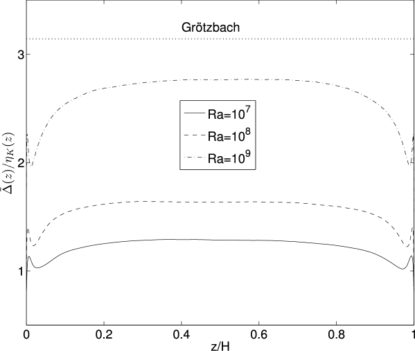
Figure 1: Ratio of the maximum geometric mean grid spacing $\tilde{\Delta}(z)$ and the Kolmogorov scale $\eta_{K}(z)$ for three different Rayleigh numbers in cells with $\Gamma=1$. The horizontal dotted line indicates the global Grötzbach resolution criterion $\Delta/\eta_{K}\leq\pi$ (Grötzbach 1983) where $\Delta$ is the global geometric mean grid spacing.

The equations are discretized on a staggered grid with a second-order finite difference scheme (Verzicco & Orlandi 1996; Verzicco & Camussi 2003). The pressure field $p$ is determined by a two-dimensional Poisson solver after applying a one-dimensional Fast Fourier Transform (FFT) in the azimuthal direction. The time advancement is done by a third-order Runge-Kutta scheme. The grid spacings are non-equidistant in the radial and vertical directions. In the vertical direction, the grid spacing corresponds to the Tschebycheff collocation points. The grid resolutions employed in all runs are listed in Table 1. The numerical effort grows with $\Gamma^{2}$ in the horizontal circular plane since the resolution at the sidewalls has to be maintained. The smallest mean scale in a turbulent flow is the Kolmogorov dissipation length which is usually defined as

$$\eta_{K}=\frac{\nu^{3/4}}{\langle\epsilon\rangle^{1/4}}\,,$$ (4)

where $\langle\epsilon\rangle$ is the mean of the energy dissipation rate (see e.g. Pope 2000), which is given by

$$\epsilon({\bm{x}},t)=\frac{\nu}{2}\left(\frac{\partial u_{i}}{\partial x_{j}}+\frac{\partial u_{j}}{\partial x_{i}}\right)^{2}.$$ (5)

The symbol $\langle\cdot\rangle$ stands for a statistical average. The resolution criteria based on $\eta_{K}$ works well in homogeneous isotropic turbulence, but has to be modified for the inhomogeneous situation. We define a height-dependent Kolmogorov scale as

$$\eta_{K}(z)=\frac{\nu^{3/4}}{\langle\epsilon(z)\rangle_{A,t}^{1/4}}\,.$$ (6)

The symbol $\langle\cdot\rangle_{A,t}$ denotes an average over a plane at a fixed height $z$ and an ensemble of statistically independent snapshots. Following Emran & Schumacher (2008), we define the maximum of the geometric mean of the grid spacing at height $z$ by $\tilde{\Delta}(z)=\max_{\phi,r}[\sqrt[3]{\Delta_{\phi}(z)\Delta_{r}(z)\Delta_{z}(z)}]$. Fig. 1 plots the ratios $\tilde{\Delta}(z)/\eta_{K}(z)$ over the cell height for three different Rayleigh numbers. One can observe that the ratio varies close to the upper and lower plates and levels off in the bulk. Overall, it does not exceed the global resolution criterion by Grötzbach (1983), $\Delta/\eta_{K}\leq\pi$, for the given Rayleigh numbers.

$N_{\phi}\times N_{r}\times N_{z}$	$Ra$	$\Gamma$	$t/t_{f}$	$Nu\pm\sigma$	$\sigma\;\;\mbox{in}\;\;\%$
$97\times 65\times 128$	$10^{7}$	0.50	300	17.08$\pm$0.07	0.4
$193\times 97\times 128$	$10^{7}$	1.00	150	16.73$\pm$0.08	0.5
$217\times 133\times 128$	$10^{7}$	1.50	111	16.37$\pm$0.08	0.5
$217\times 133\times 128$	$10^{7}$	1.75	151	16.11$\pm$0.03	0.2
$217\times 133\times 128$	$10^{7}$	2.00	250	15.88$\pm$0.07	0.4
$217\times 133\times 128$	$10^{7}$	2.25	251	15.97$\pm$0.04	0.2
$257\times 165\times 128$	$10^{7}$	2.50	251	15.77$\pm$0.03	0.1
$257\times 165\times 128$	$10^{7}$	2.75	251	15.97$\pm$0.04	0.3
$257\times 165\times 128$	$10^{7}$	3.00	150	16.06$\pm$0.05	0.3
$301\times 211\times 128$	$10^{7}$	4.00	150	16.22$\pm$0.03	0.2
$385\times 281\times 128$	$10^{7}$	6.00	150	16.66$\pm$0.04	0.2
$401\times 311\times 128$	$10^{7}$	8.00	150	17.44$\pm$0.02	0.1
$513\times 361\times 128$	$10^{7}$	10.00	150	17.34$\pm$0.03	0.2
$601\times 401\times 128$	$10^{7}$	12.00	150	17.49$\pm$0.03	0.2
$151\times 81\times 160$	$5\times 10^{7}$	0.50	150	26.20$\pm$0.21	0.8
$257\times 129\times 160$	$5\times 10^{7}$	1.00	150	25.86$\pm$0.13	0.5
$271\times 151\times 160$	$5\times 10^{7}$	2.00	149	25.83$\pm$0.12	0.5
$401\times 225\times 160$	$5\times 10^{7}$	3.00	145	25.90$\pm$0.05	0.2
$151\times 101\times 256$	$10^{8}$	0.50	300	32.06$\pm$0.24	0.7
$271\times 151\times 256$	$10^{8}$	1.00	150	32.21$\pm$0.32	1.0
$271\times 151\times 256$	$10^{8}$	1.25	150	31.77$\pm$0.15	0.5
$321\times 161\times 256$	$10^{8}$	1.50	150	31.39$\pm$0.11	0.3
$321\times 161\times 256$	$10^{8}$	1.75	249	31.57$\pm$0.10	0.3
$361\times 181\times 256$	$10^{8}$	2.00	145	31.25$\pm$0.31	1.0
$401\times 201\times 256$	$10^{8}$	2.25	143	31.25$\pm$0.21	0.7
$401\times 201\times 256$	$10^{8}$	2.50	146	31.87$\pm$0.18	0.6
$401\times 201\times 256$	$10^{8}$	2.75	145	32.34$\pm$0.08	0.3
$451\times 225\times 256$	$10^{8}$	3.00	141	32.29$\pm$0.12	0.4
$541\times 257\times 256$	$10^{8}$	4.00	132	33.20$\pm$0.08	0.2
$801\times 451\times 256$	$10^{8}$	8.00	81	34.78$\pm$0.13	0.4
$201\times 101\times 310$	$10^{9}$	0.50	150	63.67$\pm$0.56	0.9
$361\times 181\times 310$	$10^{9}$	1.00	139	64.31$\pm$0.64	1.0
$811\times 321\times 310$	$10^{9}$	2.00	109	63.25$\pm$0.26	0.4
$1025\times 551\times 310$	$10^{9}$	3.00	110	65.11$\pm$0.50	0.8

Table 1: Parameters of simulation runs. The grid resolution, Rayleigh number $Ra$, and aspect ratio $\Gamma$ are given. The Prandtl number is $Pr=0.7$ throughout this study. Furthermore, the total integration time in units of the free-fall time $t_{f}=H/U_{f}$, with $U_{f}=\sqrt{g\alpha\Delta TH}$, and the Nusselt number $Nu$ with standard deviation $\sigma$ are given. For all Rayleigh numbers, we find that a characteristic convective velocity $U_{c}=\sqrt{\langle u^{2}\rangle_{V,t}}$ is about $U_{f}/5$. Consequently, $t/t_{f}$ has to be divided by 5 in order to get $t/t_{c}$, where the alternative convective time unit is defined as $t_{c}=H/U_{c}$. This time unit was suggested by van Reeuwijk et al. (2008) since the standard free-fall velocity $U_{f}$ is too large in comparison with actual turbulent velocity fluctuations.

Fig. 2 displays the $z$-dependent mean profiles of the temperature and the product of the temperature and vertical velocity component. The variations manifested in the profiles contribute to the Nusselt number variation with $\Gamma$ . The inset magnifies the mean temperature profile for $Ra=10^{9}$ and $\Gamma=3$, where the boundary layer is resolved with 17 grid planes.

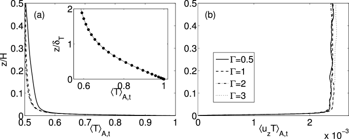
Figure 2: The $z$-dependent mean profiles of the (a) temperature and (b) product of the temperature and vertical velocity component. Data for four aspect ratios are plotted at Rayleigh number $Ra=10^{9}$. The inset in (a) magnifies the mean temperature profile in the thermal boundary layer for the simulation at $Ra=10^{9}$ and $\Gamma=3$. Profiles are shown for the lower half ($0\leq z/H\leq 0.5$) of the cell only due to symmetry.

III Dependence of the global heat transfer on aspect ratio

III.1 $Nu(\Gamma)$ at fixed Rayleigh number $Ra$

The heat transfer through each plane at a fixed height $z$ following the averaging of Eq. (3) with respect to the horizontal plane is given by

$$Nu(z)=\frac{\langle u_{z}T\rangle_{A,t}-\kappa\partial_{z}\langle T\rangle_{A,t}}{\kappa\Delta T/H}=const.$$ (7)

The global Nusselt number, $Nu$, can then be written as

$$Nu=\frac{1}{H}\int_{0}^{H}Nu(z)\mbox{d}z=1+\frac{H}{\kappa\Delta T}\langle u_{z}T\rangle_{V,t}\,,$$ (8)

where $\langle\cdot\rangle_{V,t}$ denotes an average over the whole cell volume and an ensemble of statistically independent snapshots. The samples are gathered over the total integration time, which is also listed in Table 1, and given in units of the free-fall time $t_{f}=H/U_{f}$, with the free-fall velocity $U_{f}=\sqrt{g\alpha\Delta TH}$ as the characteristic velocity. The last columns of the table display the Nusselt number $Nu$ and the standard deviation $\sigma$, which is calculated as

$$\sigma=\sqrt{\frac{1}{N_{z}}\sum^{N_{z}}_{j=1}[Nu(z_{j})-Nu]^{2}}\,.$$ (9)

Here $z_{j}$ is the vertical coordinate of each gridplane and $Nu(z)$ and $Nu$ follow from Eqns. (7) and (8), respectively. These standard deviations are smaller than or equal to 1% and thus comparable with Kerr (1996). The total integration time of the simulations is comparable with van Reeuwijk et al. (2008).

Fig. 3 shows the Nusselt number $Nu$ as a function of the aspect ratio, $\Gamma$, for three different Rayleigh numbers, namely $Ra=10^{7},10^{8}$ and $10^{9}$. At $Ra=10^{7}$ (Fig. 3(a)), $Nu$ decreases with increasing $\Gamma$, attains a minimum value at $\Gamma\approx 2.5$, then increases to a maximum value close to $\Gamma\approx 8$, and finally saturates for $\Gamma>8$. Variations of $Nu(\Gamma)$ can also be observed in Figs. 3(b) and 3(c) for the other two larger Rayleigh numbers. The minimum of $Nu(\Gamma)$ is detected at $\Gamma\approx 2.5$ and $\Gamma\approx 2.25$ for $Ra=10^{7}$ and $Ra=10^{8}$, respectively. This is the point where a transition in the LSC from a single-roll to a double-roll pattern will occur (see section 4). On the basis of stability analysis, Oresta et al. (2007) have shown that there is always a single-roll for $\Gamma\leq 2$ in the weakly nonlinear regime irrespective of the initial conditions. However, our Rayleigh numbers here are in fully turbulent regime. With our present computing capability, we could not go beyond $\Gamma>8$ for $Ra=10^{8}$ and $\Gamma>3$ for $Ra=10^{9}$. In particular, for the largest Rayleigh number, we can provide four data points only and, therefore, the minimum of $Nu(\Gamma)$ is inconclusive in this case, although it is apparently at $\Gamma\approx 2$ in Fig. 3(c). On the basis of our simulation data, we can not conclude exactly at which aspect ratio the Nusselt numbers become independent of the cell geometry for all the Rayleigh numbers, however, the trend indicates that it is at $\Gamma\approx 8$ for $Ra=10^{7}$ and $\Gamma\gtrsim 8$ for $Ra=10^{8}$. The variations in $Nu$, as defined by the difference between the maximum and minimum in the Nusselt number series, are significant – especially for the lower Rayleigh numbers – and yield 10.9%, 11.3%, and 3.0% for $Ra=10^{7}$, $10^{8}$ and $10^{9}$ respectively.

A closer inspection of the three panels in Fig. 3 reveals non-monotonic graphs of $Nu(\Gamma)$ with local maxima and minima, in particular for the two larger Rayleigh numbers. We have first verified that there is sufficient statistical convergence of the data (see Table 1). Since statistical uncertainties can be excluded, there must be physical reasons for the behaviour observed in Fig. 3. We observe that the time-averaged flow patterns in the turbulent cell are similar to those at the onset of convection (Figs. 5 and 6). In this case, an integer number of rolls must fit into the cell. This is exactly the reason why, for example, the linear instability studies by Koschmieder (1969) and Charlson & Sani (1970, 1971) in the cylindrical cells with insulated side-walls yield stability curves $Ra_{cr}(\Gamma)$ with local extrema in the low–$\Gamma$ regime, and extend to an asymptotic value for larger $\Gamma$ only. Small discontinuities in $Nu(Ra)$ in the weakly nonlinear regime, which could be traced back to a change of the number of rolls in the cell, have been also reported by Gao et al. (1987).

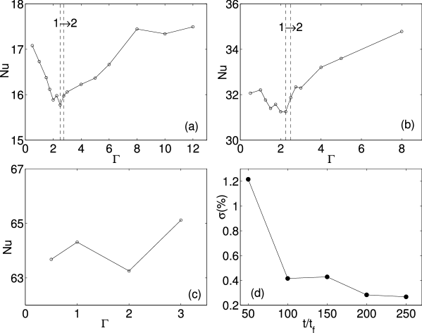
Figure 3: Nusselt number $Nu$ as a function of the aspect ratio $\Gamma$ for (a) $Ra=10^{7}$, (b) $Ra=10^{8}$, (c) $Ra=10^{9}$. The crossover from one circulation roll to two rolls is indicated in (a) and (b) by two parallel dashed lines. The errorbars for all Nusselt numbers shown are smaller than the size of the symbols. For each single snapshot, the Nusselt number was determined as a volume average. In addition, an arithmetic mean is taken over $N_{samp}=t/t_{f}$ statistically independent turbulent samples (see Eq. (8) and Table 1). The convergence of the standard deviation $\sigma$ with increasing number of samples $N_{samp}=t/t_{f}$ is shown in (d) for the data set $Ra=10^{7}$ and $\Gamma=2$.

These pattern bifurcations can be studied when a small number of degrees of freedom dominates the dynamics. It is not obvious that in a fully turbulent case, where infinitely many degrees of freedom exist, coherent patterns exist and prevail. Similar patterns can, however, be found in a turbulent Taylor vortex flow at high Reynolds number (Lathrop et al. 1992). The POD analysis in section 5 demonstrates that the LSC carries a significant amount of heat through the cell. We also show that a change of the LSC morphology causes jumps in the amount of heat transported by the first few POD modes. These findings strengthen our observation of $\Gamma$-dependent heat transfer (see Fig. 3). It should also be mentioned that persistent coherent patterns at larger Rayleigh numbers have been emphasized by Busse (2003) as a sequence-of-bifurcations to the turbulent state.

III.2 $Nu(Ra)$ at fixed aspect ratio $\Gamma$

Systematic experiments with various values of $\Gamma$ larger than unity were conducted by three groups. First, Wu & Libchaber (1992) detected a power law scaling with $Ra$, namely

$$Nu(Ra,\Gamma)=A(\Gamma)\times Ra^{\beta}\,.$$ (10)

Their measurements indicated almost an unchanged exponent $\beta$ and an aspect-ratio-dependent prefactor. Second, Sun et al. (2005) suggested the following scaling law on the basis of their experiments as

$$Nu(Ra,\Gamma)=A_{1}(\Gamma)\times Ra^{\beta_{1}}+A_{2}(\Gamma)\times Ra^{\beta_{2}}\,.$$ (11)

This scaling is a combination of two power laws with $\beta_{1}=1/3$ and $\beta_{2}=1/5$. Again, the prefactors depend on $\Gamma$ and a saturation of the Nusselt number $Nu$ for $\Gamma\geq 10$ has been detected. Third, Funfschilling et al. (2005) did not observe any sensitivity of the heat transfer on the aspect ratio. Their measurements gave power laws of the form

$$Nu(Ra,\Gamma)=A\times Ra^{\beta}\,,$$ (12)

but with a continuous drift of the exponent from $\beta=0.28$ at $Ra\sim 10^{8}$ up to $\beta=0.33$ at $Ra\gtrsim 10^{10}$. Their results were essentially unaltered by an increase in the aspect ratio. On the numerical side, a power law of $Nu\sim\Gamma^{-1}$ for $\Gamma\leq 3$ was obtained by Ching & Tam (2006) on the basis of two-dimensional steady state calculations.

The present data allows us to compare our results with the scaling laws given in (10)–(12). Table 2 displays the fit results for power laws in the form $Nu=A\times Ra^{\beta}$ at fixed aspect ratios $\Gamma=1/2,1,2$ and 3. Each data series contains four Rayleigh numbers, namely $Ra=10^{7}$, $5\times 10^{7}$, $10^{8}$ and $10^{9}$. Within this range of $Ra$, we observe a growth of the exponent $\beta$ from 0.287 to 0.305, which is about 6% variation. The present scaling law for $\Gamma=1$ differs slightly from the earlier reported scaling of $Nu=0.175\times Ra^{0.283}$ in Emran & Schumacher (2008). In the former case, six Rayleigh numbers from $5\times 10^{6}$ to $10^{9}$, but fewer snapshots for the higher Rayleigh numbers, were included. This demonstrates the sensitivity of the scaling laws and demands additional efforts to be taken here. Both the prefactor $A$ and exponent $\beta$ seem to be functions of the aspect ratio and the functional form is thus

$$Nu(Ra,\Gamma)=A(\Gamma)\times Ra^{\beta(\Gamma)}\,.$$ (13)

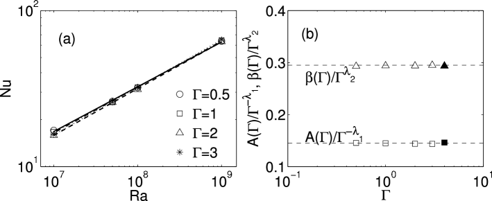
Figure 4: Aspect ratio dependence of the fit coefficients, $A(\Gamma)$ and $\beta(\Gamma)$. (a): Data for the Nusselt number and power law fits to $Nu(Ra)$ as reported in Table 2. (b): Compensated power law plots for $A(\Gamma)$ and $\beta(\Gamma)$. The exponents are $\lambda_{1}=0.18$ for $A$ and $\lambda_{2}=0.03$ for $\beta$. The open symbols are the present simulation data. The filled symbols correspond to Niemela & Sreenivasan (2006). We have fitted their data from $Ra=1.10\times 10^{8}$ to $9.51\times 10^{9}$ (see their Table 1).

Fig. 4(a) shows power law fits (13) to our DNS data for several aspect ratios and Fig. 4(b) shows $A(\Gamma)\sim\Gamma^{-\lambda_{1}}$ and $\beta(\Gamma)\sim\Gamma^{\lambda_{2}}$ in a compensated form for $0.5\leq\Gamma\leq 3$. The measurements that come closest to the present study, both in Rayleigh and Prandtl numbers, are those by Niemela & Sreenivasan (2006) at $\Gamma=4$. A power law fit of their data for $1.10\times 10^{8}\leq Ra\leq 9.51\times 10^{9}$ yields $Nu=0.114\times Ra^{0.306}$. Adding these parameters to Fig. 4 covers data over almost a decade of $\Gamma$. We see that both parameters, $A$ and $\beta$, almost perfectly follow the power law with respect to $\Gamma$. The exponent for $\beta$ is $\lambda_{2}=0.03$, which is small. The dependence of the prefactor $A$ on $\Gamma$ is stronger, with $\lambda_{1}=0.18$. It is clear that further studies are required to determine whether this weak dependence on $\Gamma$ prevails at larger Rayleigh numbers or not. Furthermore, we can expect that, for sufficiently large $\Gamma$, both exponents will saturate to aspect-ratio-independent values. This was shown clearly in Fig. 3 for $Ra=10^{7}$. In addition, the saturation threshold for $A$ and $\beta$ most likely depends on the Prandtl number, which is constant in our case.

Fit Coefficients	$\Gamma=\frac{1}{2}$	$\Gamma=1$	$\Gamma=2$	$\Gamma=3$
$A$	$0.165$	$0.145$	$0.127$	$0.118$
$\beta$	$0.287$	$0.294$	$0.300$	$0.305$

Table 2: Nusselt number as a function of the Rayleigh number for different aspect ratios. The scaling $A\times Ra^{\beta}$ has been fit for four aspect ratios.

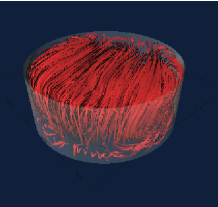
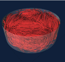
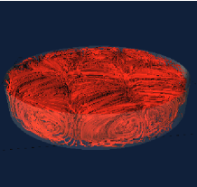
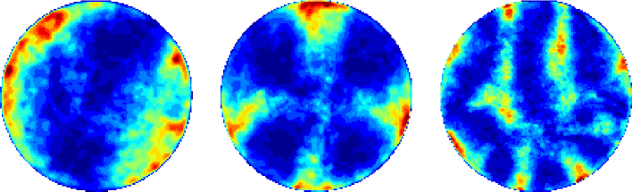
Figure 5: Flow patterns at different aspect ratios. Streamlines (top row) and contours of the local heat transfer $u_{z}\theta$ (bottom row) for three different aspect ratios, $\Gamma=2.5$ (left column), $\Gamma=3$ (middle column), and $\Gamma=6$ (right column), at $Ra=10^{7}$ are presented. All data are obtained by time averaging a sequence of 50 statistically independent snapshots. In the bottom row $\langle u_{z}\theta\rangle_{t}(r,\phi,z=1/2)$ is shown.

IV Large-scale circulation

Let us now investigate the behaviour of the LSC. In Fig. 5, we present the LSC for three aspect ratios $\Gamma=$2.5, 3, and 6 at $Ra=10^{7}$. The streamline plots in the upper three panels have been obtained by averaging the velocity field over 50 consecutive snapshots. These snapshots are separated from each other by $\Delta t=t_{f}=H/U_{f}$. Averaging over three disjoint sequences of 50 snapshots leaves the observed LSC patterns unchanged. We conclude, therefore, that the detected LSC pattern is not transient. Transient behaviour and large-scale saturation have been investigated by von Hardenberg et al. (2008). The time-averaging over the coarse sequence of snapshots removes not only all small-scale fluctuations of the velocity field, but also oscillations of the LSC, which have been observed in recent experiments (e.g. Xi & Xia (2008) and Brown & Ahlers (2008)), mostly for $\Gamma\leq 1$. Between $\Gamma=2.5$ and 2.75, the system bifurcates from a one-roll to a two-roll pattern. We have also identified this crossover in LSC between $2.25<\Gamma<2.5$ for $Ra=10^{8}$. However, for $Ra=10^{9}$ we have noticed a single-roll circulation pattern at $\Gamma=2$ and a triple-roll pattern at $\Gamma=3$. Here, the LSC patterns for aspect ratios between 2 and 3 were not investigated for the highest Rayleigh number. A single-roll at $\Gamma=2$ is consistent with the findings of Sun et al. (2005), Oresta et al. (2007) and Bukai et al (2009). The crossovers of the LSC are marked in Fig. 3(a) and Fig. 3(b) by two parallel dashed lines. With increasing aspect ratio, the LSC becomes a more complex multi-roll configuration, as can be seen in the third column of Fig. 5 for $\Gamma=6$.

In the lower row of Fig. 5, we show the corresponding contour plots of $\langle u_{z}\theta\rangle_{t}$ at the midplane where

$$\theta({\bm{x}},t)=T({\bm{x}},t)-\langle T(z)\rangle_{A,t}\,.$$ (14)

The quantity $u_{z}\theta$ is the local convective heat flux contribution and $u_{z}\theta>0$ if rising and falling plumes are present. The appearance of rising and falling plumes (red in $\langle u_{z}\theta\rangle_{t}$ contours) in the three panels (lower row of Fig. 5) is directly correlated to the corresponding LSC pattern of the time averaged velocity field. We have also verified that almost the same pattern holds for the fluctuations of the local heat transfer, as given by $\langle(u_{z}\theta)^{2}\rangle_{t}$.

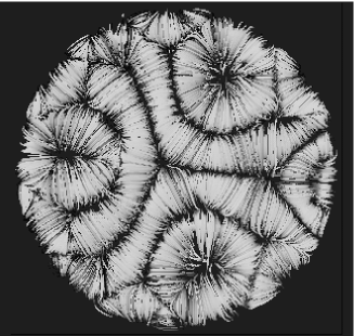
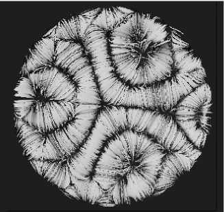
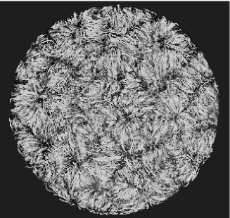
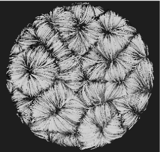
Figure 6: Top view of the large scale circulation (LSC) patterns at $\Gamma=12$ for two different Rayleigh numbers, $Ra=6\times 10^{3}$ (top row) and $Ra=10^{7}$ (bottom row). The streamlines of the instantaneous (left column) and time-averaged (right column) velocity field are shown here. In both cases, the time averaging is done over 50 convective time units $t_{f}$.

As already indicated in Fig. 5, the LSC becomes more complex when the aspect ratio becomes larger. For Rayleigh number $10^{7}$, we were able to run a numerical simulation up to $\Gamma=12$. Fig. 6 reveals such a complex LSC pattern in convective flow for two different Rayleigh numbers, $Ra=10^{7}$ and $Ra=6000$, at $\Gamma=12$. The left column shows the top view of the streamlines for instantaneous snapshots of both simulations, while the right column shows the time-averaged velocity field as in Fig. 5. When the small-scale turbulence (see lower left panel) is filtered out, the resulting pattern is strikingly similar to the weakly nonlinear regime right above the onset of convection. We observe extended rolls and pentagon-like cells. These patterns have been reported, for example, in experiments by Croquette (1989) with argon at $Pr=0.69$ for Rayleigh numbers $Ra\approx 2Ra_{c}$, where $Ra_{c}$ is the critical Rayleigh number of the onset of convection. Fig. 7 adds further support to the Rayleigh-number-dependence of the LSC. The left panel nicely displays the extended roll patterns in the weakly nonlinear regime at $Ra=6000$ and $\Gamma=8$. Relics of these patterns are still present in the turbulent regime at $Ra=10^{7}$ (mid panel). For the largest Rayleigh number, $Ra=10^{8}$, the LSC is transformed into a pentagon-like cell structure. Similarly, if we compare the top-right panel of Fig. 6 with the left panel of Fig. 7, we see that there is a reorganization of flow from the roll shape to pentagonal or hexagonal structures with increasing $\Gamma$ for a fixed $Ra$.

Regular patterns in the turbulent convection regime were studied in detail by Fitzjarrald (1976) in a square cell filled with air for aspect ratios between 2 and 58 covering a range of Rayleigh numbers between $4\times 10^{4}$ and $7\times 10^{9}$. He calculated the dominant horizontal scales from the Fourier co-spectra of $u_{z}$ and $T$. The spectral peak in the heat flux corresponds to a wavelength $\Lambda$ that increased from $4H$ to $6H$ for $4\times 10^{4}<Ra<1.7\times 10^{7}$ and thus $58>\Gamma>15$. Based on Figs. 5 and 6 for $Ra=10^{7}$ and Fig. 7 for $Ra=10^{8}$, we take the width of the large-scale circulation roll (which corresponds to the spacing between local maxima of $\langle u_{z}\theta\rangle$) as $\Lambda/2$ and get thus a wavelength $\Lambda\approx 4H$ for $\Gamma=6,8$ and 12. The associated wavenumber $k=2\pi/\Lambda\approx 1.5H^{-1}$ which is about half the size of $k_{c}=3.117H^{-1}$ at the onset of thermal convection in an infinite layer. The dominant horizontal scales are similar to those of Fitzjarrald. The results in Fig. 5 further confirm the observation made by Fitzjarrald. This wavelength shrinks at smaller aspect ratios where the pattern has to fit into the cylindrical cell. Hartlep et al. (2005) have also traced back their large-scale turbulent temperature patterns to the states which are observed in the weakly nonlinear regime. A series of simulations at $\Gamma=10$ for Rayleigh numbers up to $Ra=10^{7}$ confirms a characteristic wavelength of half their box size, i.e. $\Lambda\approx 5H$ for $Pr=0.7$. This wavelength was $\Lambda\approx 3H$ at $Ra=4000$. Their study shows in addition a clear shape dependence of the circulation rolls on the Prandtl number. Slight variations of $\Lambda$ in the three studies might be caused by different cell geometries and boundary conditions in the simulations. Nevertheless, the same range of wavelengths can be observed for $Ra\sim 10^{7}$ and $Pr=0.7$ in all works.

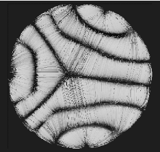
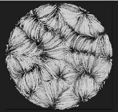
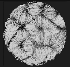
Figure 7: Rayleigh number dependence of the large scale circulation. Left panel: $Ra=6000$. Mid panel: $Ra=10^{7}$. Right panel: $Ra=10^{8}$. All data are for $\Gamma=8$.

Although qualitative similarities between the LSC patterns at small $Ra$ and those at higher $Ra$ are obvious from Fig. 6, we can expect that the particular mechanisms that drive the large-scale flow will be different. The onset of a flow motion for small $Ra$ is triggered by a slight dominance of buoyancy forces per unit mass, $f_{b}=g\alpha\theta$, compared to the restoring drag forces per unit mass, $f_{d}=\frac{1}{2}C_{f}u_{z}^{2}H$. This is the simple chaotic waterwheel picture by Malkus and Howard (see Strogatz 1994). In the turbulent case, the heat transport through the thin thermal boundary layers is responsible for large-scale spatial temperature differences. Spatial temperature differences create pressure gradients which drive the large-scale flow (Reeuwijk et al. 2008). This might the reason why the wavelength of the circulation rolls is slightly increasing with growing $Ra$.

We can summarise that, for the range of parameters covered here, the LSC patterns do not disappear in the turbulent regime up to $Ra=10^{9}$. For the larger aspect ratios pentagon-like circulation cells are formed preferentially.

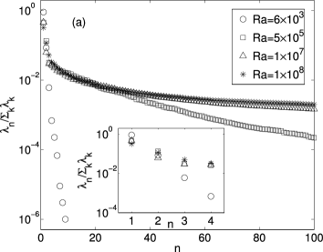
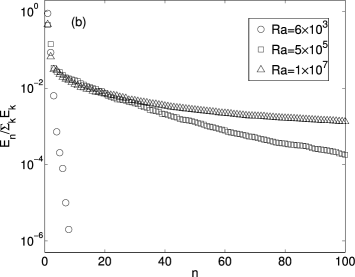
Figure 8: (a) Normalized POD eigenvalue spectrum of the total energy (thermal plus kinetic) is shown for four different Rayleigh numbers as indicated in the legend. (b) Normalized POD eigenvalue spectrum of the kinetic energy is shown for three different Rayleigh numbers as indicated in the legend. The snapshot method was conducted over 100 state vectors. The aspect ratio is $\Gamma=3$ in all four cases. The spectra in (a) and (b) coincide almost perfectly. The inset magnifies the spectra for the first few modes.

V Proper Orthogonal Decomposition of the turbulent convection flow

V.1 The snapshot method

The turbulent heat transfer is the sum of transfers by the LSC and the turbulent fluctuations. In order to disentangle both contributions systematically, we conduct a so-called Karhunen-Loève method or Proper Orthogonal Decomposition (POD). The reader is referred to Smith et al. (2005) for a compact tutorial on this subject. Here, we outline the basic ideas only. The application of the POD method to the convection problem goes primarily back to Sirovich and his co-workers (see e.g. Sirovich & Park 1990). Consider a state vector ${\bm{v}}=({\bm{u}},\theta)$ with zero mean, $\langle{\bm{v}}\rangle=0$. It has a mean turbulent energy (kinetic energy plus temperature variance), which is given by

$$E=\langle({\bm{v}},{\bm{v}})\rangle=\Big{\langle}\int_{V}\sum_{k=1}^{4}v_{k}({\bm{x}},t)v_{k}({\bm{x}},t)\,\mbox{d}^{3}x\Big{\rangle}_{t}\,,$$ (15)

where $V$ is the cell volume and the scalar product $(\cdot,\cdot)$ is defined in $L_{2}(V$). At the core of the method is the determination of the POD modes ${\bm{\phi}}({\bm{x}})$, which maximize the following functional

$$\frac{\langle|({\bm{v}},{\bm{\phi}})|^{2}\rangle_{t}}{({\bm{\phi}},{\bm{\phi}})}\rightarrow\mbox{max}.$$ (16)

Variational calculus then yields the following integral equation

$$\int_{V}\hat{\bm{K}}({\bm{x}},{\bm{x}}^{\prime}){\bm{\phi}}^{(m)}({\bm{x}}^{\prime})\,\mbox{d}^{3}x^{\prime}=\lambda_{m}{\bm{\phi}}^{(m)}({\bm{x}}),$$ (17)

with the kernel (or covariance matrix) $K_{ij}({\bm{x}},{\bm{x}}^{\prime})=\langle v_{i}({\bm{x}},t)v_{j}({\bm{x}}^{\prime},t)\rangle_{t}$ and $i,j=1,2,3,4$. If the kernel is a Hermitian and non-negative operator, the set of empirical eigenfunctions $\{{\bm{\phi}}^{(m)}\}$ forms an orthonormal system, i.e. $({\bm{\phi}}^{(m)},{\bm{\phi}}^{(n)})=\delta_{mn}$. The integral equation is transformed into a matrix eigenvalue problem. In our case the size of the kernel becomes extremely large, namely a $4N\times 4N$ matrix for ${\bm{v}}=({\bm{u}},\theta)$ and $N=N_{r}\times N_{\phi}\times N_{z}$. Symmetries and incompressibility of the flow reduce the number of degrees of freedom in many cases. However, we still have to apply the method of snapshots, which is the preferred choice if $N\gg N_{T}$, with $N_{T}$ the number of snapshots. We therefore construct empirical eigenfunctions as a linear combination of the state vectors ${\bm{v}}$, where the eigenfunctions are given by

$${\bm{\phi}}^{(m)}({\bm{x}})=\sum_{i=1}^{N_{T}}\alpha_{i}^{(m)}{\bm{v}}({\bm{x}},t_{i})\,.$$ (18)

Such a procedure reduces the complexity of the problem and leads to the solution of an eigenvalue problem of $N_{T}\times N_{T}$ matrix, as is evident from the subsequent expressions. If $\langle\cdot\rangle_{t}$ is substituted by an arithmetic mean over the snapshots, it follows from (17) that

$$\frac{1}{N_{T}}\int_{V}\sum_{k=1}^{N_{T}}v_{p}({\bm{x}},t_{k})v_{n}({\bm{x}}^{\prime},t_{k})\phi_{n}^{(m)}({\bm{x}}^{\prime})\,\mbox{d}^{3}x^{\prime}=\lambda_{m}\phi_{p}^{(m)}({\bm{x}}).$$ (19)

With (18) one can arrive at

$$\sum_{k=1}^{N_{T}}v_{p}({\bm{x}},t_{k})\left[\sum_{i=1}^{N_{T}}\frac{1}{N_{T}}\int_{V}v_{n}({\bm{x}}^{\prime},t_{k})v_{n}({\bm{x}}^{\prime},t_{i})\,\mbox{d}^{3}x^{\prime}\,\alpha_{i}^{(m)}\right]=\sum_{q=1}^{N_{T}}v_{p}({\bm{x}},t_{q})\lambda_{m}\alpha_{q}^{(m)}\,,$$ (20)

and thus

$$\sum_{i=1}^{N_{T}}\frac{1}{N_{T}}({\bm{v}}(t_{k}),{\bm{v}}(t_{i}))\alpha_{i}^{(m)}=\sum_{i=1}^{N_{T}}C_{ki}\alpha_{i}^{(m)}=\lambda_{m}\alpha_{k}^{(m)}\,.$$ (21)

Eventually, $N_{T}$ eigenvectors $\{{\bm{\alpha}}^{(m)}\}$, with $m=1,2,...,N_{T}$, represent $N_{T}$ POD modes $\{{\bm{\phi}}^{(m)}\}$ (vectors of $4N$ components) constructed from the state vectors.

We proceed in two different steps. First, we use ${\bm{v}}={\bm{u}}$ only and not the combined velocity-temperature state vectors. The eigenvalue spectrum $E_{1}\geq E_{2}\geq\dots E_{N_{T}}$ then quantifies the fraction of the turbulent kinetic energy contained in each of the $N_{T}$ POD modes. Second, we use ${\bm{v}}=({\bm{u}},\theta)$ and determine the total energy spectrum $\lambda_{1}\geq\lambda_{2}\geq\dots\lambda_{N_{T}}$. The latter will be used in the subsequent sections. Both eigenvalue spectra are presented in Fig. 8 for different Rayleigh numbers and $N_{T}=100$ snapshots. At the smallest Rayleigh number $Ra=6\times 10^{3}$, the first few POD modes contain most of the total energy (Fig. 8(a)) and kinetic energy (Fig. 8(b)). This is the weakly nonlinear regime of convection. With increasing Rayleigh number, the spectra decay slowly. For Rayleigh numbers $Ra\geq 10^{7}$ the convection is turbulent and a significant fraction of the kinetic and total energy is distributed among the higher-order POD modes. The inset in Fig. 8(a) shows the magnified view for the first few POD modes. This observation is in agreement with Sirovich & Park (1990). The dynamic significance of the subsequent modes increases steadily with increasing Rayleigh number since turbulent fluctuations are present.

V.2 Spatial structure of primary and secondary modes

Before we proceed to the analysis of the turbulent heat transfer, we visualize the spatial structure of the first two POD modes and compare it with the LSC. Fig. 9 shows the three-dimensional view of the primary and secondary modes. The velocity field ($\phi_{1}^{(m)}({\bm{x}}),\phi_{2}^{(m)}({\bm{x}}),\phi_{3}^{(m)}({\bm{x}}))$ with $m=1,2$, is plotted as streamlines in the left column and the temperature field $\phi_{4}^{(m)}({\bm{x}})$ at two isolevels is plotted in the right column. The data set corresponds to $\Gamma=3$ and $Ra=10^{7}$. The structure of the velocity field of the primary mode almost exactly replicates the time-averaged velocity field shown in Fig. 5. This replication is also verified for other aspect ratios, which are not shown here. The shape of the primary temperature POD mode indicates hot up- and cold downwellings on the side wall. The two lower panels of Fig. 9 show that the secondary modes exhibit a more complex structure. The primary and secondary POD mode have the same number of large-scale rolls. In addition, we detect smaller substructures of the secondary modes, such as recirculation vortices close to the top and bottom plates and weak modulations of the large-scale rolls.

V.3 Heat transfer by different POD modes

The contribution of different subsets of the POD modes to the turbulent heat transfer is determined as follows. We can decompose turbulent snapshots as

$$u_{i}({\bm{x}},t) = \sum_{m=1}^{N_{T}}a_{m}(t)\phi_{i}^{(m)}({\bm{x}})\,,$$ (22)

$$\theta({\bm{x}},t) = \sum_{m=1}^{N_{T}}a_{m}(t)\phi_{4}^{(m)}({\bm{x}})\,,$$ (23)

with $i=1,2,3$ (or $x,y,z$). The coefficients $a_{m}(t)$ correspond to the projection of the turbulent flow field at time $t$ to mode ${\bm{\phi}}^{(m)}({\bm{x}})$, which are calculated from the scalar product in $L_{2}(V)$. The Nusselt number definition (8) then translates to

$$Nu(N_{T}) = 1+\frac{H}{\kappa\Delta T}\sum_{m,n=1}^{N_{T}}\Big{\langle}a_{m}(t)\phi_{3}^{(m)}({\bm{x}})\left[\overline{T}(z)+a_{n}(t)\phi_{4}^{(n)}({\bm{x}})\right]\Big{\rangle}_{V,t}$$ (24)

$$= 1+\frac{H}{\kappa\Delta T}\sum_{m,n=1}^{N_{T}}\Big{\langle}a_{m}(t)\phi_{3}^{(m)}({\bm{x}})a_{n}(t)\phi_{4}^{(n)}({\bm{x}})\Big{\rangle}_{V,t}$$

$$= 1+\frac{H}{\kappa\Delta T}\sum_{m=1}^{N_{T}}\lambda_{m}\Big{\langle}\phi_{3}^{(m)}({\bm{x}})\phi_{4}^{(m)}({\bm{x}})\Big{\rangle}_{V}\,,$$

where $\overline{T}(z)=\langle T(z)\rangle_{A,t}$. The contribution of the mean profile drops out.

In Fig. 10, we report the contribution of various POD modes to the global heat transfer for $Ra=10^{7}$ and $10^{8}$. The contribution of the primary and secondary modes is displayed in panels (a) and (b). The expansion (24) is then truncated after 1, 2, 5, 20, and 100 POD modes. Panels (c) and (d) show the accumulated fraction to the heat transfer for the number of modes as given in the legend of both figures. As a consistency check, we compare the full expansion which is based on 100 snapshots with the Eulerian value as determined in section 3. Computational resources limit the present analysis to $N_{T}=100$ since intensive data in- and output is required. The values of $Nu$ still deviate slightly from those in Tab. 1. It is found that the convergence is slow in particular for the higher-order modes. The slow convergence was also underlined in Fig. 3(d). In Tab. 3 we have listed in addition some quantitative details of the POD analysis of the heat transfer. The results are consistent with the Eulerian values in Tab. 1.

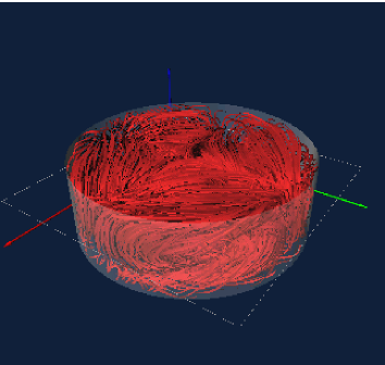
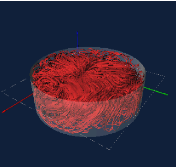
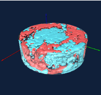
Figure 9: Three-dimensional visualization of the first two POD modes for $Ra=10^{7}$ and $\Gamma=3$. Upper row: Streamlines of the primary flow mode $(\phi_{1}^{(1)},\phi_{2}^{(1)},\phi_{3}^{(1)})$ (left) and isosurfaces of the primary temperature mode $\phi_{4}^{(1)}$ (right) at the isolevels $\pm 0.5\Delta T$. Lower row: Streamlines of the secondary flow mode $(\phi_{1}^{(2)},\phi_{2}^{(2)},\phi_{3}^{(2)})$ (left) and isosurfaces of the secondary temperature mode $\phi_{4}^{(2)}$ (right) at the isolevels $\pm 0.095\Delta T$. Blue isosurfaces correspond to negative values and red isosurfaces to positive values in both figures.

The primary POD mode carries the following fraction of the global heat transfer

$$Nu(N_{T}=1)=1+\frac{\lambda_{1}H}{\kappa\Delta T}\Big{\langle}\phi_{3}^{(1)}\phi_{4}^{(1)}\Big{\rangle}_{V}\,.$$ (25)

$Ra$	$10^{7}$					$10^{8}$
$\Gamma$	0.5	1.0	2.0	2.5	3.0	0.5	1.0	2.0	2.5	3.0
$Nu$	17.08	16.73	15.88	15.77	16.06	32.06	32.21	31.25	31.87	32.29
$Nu(N_{T}=100)$	16.74	16.42	15.28	15.26	15.42	31.13	31.78	30.64	30.88	31.05
$\frac{Nu-Nu(N_{T}=100)}{Nu}$	2.0%	1.8%	3.8%	3.3%	4.0%	2.9%	1.3%	1.9%	3.1%	3.8%
$\frac{Nu(N_{T}=1)}{Nu(N_{T}=100)}$	30%	46%	51%	47%	55%	27%	47%	51%	63%	41%

Table 3: Turbulent heat transport of POD modes. The Nusselt number $Nu$ of the analysis of the DNS data (taken from Table 1) is compared with that obtained from a sequence of $N_{T}=100$ snapshots denoted by $Nu(N_{T}=100)$. Furthermore, the contribution of the primary mode, $Nu(N_{T}=1)$, is compared to the total transport, $Nu(N_{T}=100)$.

Figure 10: Contribution of various POD modes (as indicated in the legend) to the global heat transfer for two Rayleigh numbers and five different aspect ratios. (a) Contribution of the primary and secondary modes for $Ra=10^{7}$. (b) Contribution of the primary and secondary modes for $Ra=10^{8}$. (c) Accumulated contributions for $Ra=10^{7}$. (d) Accumulated contributions for $Ra=10^{8}$. For completeness we also add the original Eulerian values of the Nusselt number.

Figure 11: Time dependence of $a_{i}(t)$ for $\Gamma=2$. The snapshots are therefore projected on the primary $(i=1)$, secondary $(i=2)$, and tertiary mode $(i=3)$. (a) $Ra=10^{7}$. (b) $Ra=10^{8}$.

For flow patterns with a single-roll circulation, i.e. $\Gamma=$ 1, 2, and 2.5 for $Ra=10^{7}$ and $\Gamma=$1 and 2 for $Ra=10^{8}$, the contribution to the heat transfer by the primary POD mode is about the same. It makes up about one half of the total amount. This contribution increases by 10% due to the transition from a single-roll to a double-roll pattern between $\Gamma=$ 2.5 and 3 for $Ra=10^{7}$. The double-roll LSC can carry more heat through the cell since the number of up- and downwelling regions with $\langle u_{z}\theta\rangle_{t}>0$ increases across the cell. This can also be seen in the plots in the lower row of Fig. 5. One can consider the dynamics around $\Gamma=2.5$ as a bottleneck for the heat transfer. The one-roll pattern gets ever flatter with increasing $\Gamma$ and can thus transfer heat less efficiently through the cell. Once the two-roll pattern is established, this bottleneck is removed and the share of the primary mode in the total heat transfer increases. The same transition appears between aspect ratios of 2 and 2.5 for $Ra=10^{8}$. Again, we detect a jump of the primary mode contribution by 12%. The opposite is the case for the slender cell at $\Gamma=0.5$. One observes a much lower $Nu$ fraction due to the primary mode in comparison to the cases with $\Gamma\geq 1$. This can be attributed to the complex flow configuration in the slender cell, in which there are either two counter-rotating rolls on top of each other, or one slender roll (Verzicco & Camussi 2003, Xi & Xia 2008a).

The secondary and higher-order modes provide information that can be obtained within the present POD analysis only. The fraction of the secondary POD mode (see Fig. 10 (a) and (b)) to the global heat transfer is much smaller than that of the primary. It is about 5% for the larger aspect ratios and remains almost insensitive when the primary mode switches from a one-roll to a two-roll pattern. A closer inspection of both plots suggests, however, that an increase of the portion of the total heat transfer due to the primary mode causes a decrease of that of the secondary mode. This is clearly indicated for $\Gamma=0.5$ and 1 in both $Ra=10^{7}$ and $10^{8}$ series, and for $\Gamma=2$, 2.5 and 3 in the series with $Ra=10^{8}$. It further supports our arguments in the last paragraph. The local minimum of the secondary POD mode contribution coincides with the local maximum of the primary one. When the primary mode becomes less efficient in transferring heat, the secondary mode has to take a bigger share. The two panels in Fig. 11 display finally the time dependence of the expansion coefficients of the first three POD modes, $a_{m}(t)$ with $m=1,2,3$. The graphs are obtained by projecting the 100 snapshots onto the POD modes $\phi_{i}^{(m)}({\bm{x}})$ for $m=1,2,3$. While the primary modes remains nearly constant, we see that the secondary and tertiary modes oscillate with a period of approximately $30t_{f}$ and are shifted with respect to each other by about $10t_{f}$. The secondary and tertiary mode contribute thus mainly to temporal variance of the heat transfer. Their time-averaged contributions remain, however, significantly lower than that of the primary mode.

VI Summary and discussion

Within the parameter range of the present study, the DNS results have revealed a dependence of the Nusselt number on the aspect ratio. The variation in $Nu(\Gamma)$ curve is between 11% and 3%, depending on the Rayleigh number and the range of accessible aspect ratios. A minimum of $Nu(\Gamma)$ is found at $\Gamma\approx 2.5$ and $\Gamma\approx 2.25$ for $Ra=10^{7}$ and $Ra=10^{8}$, respectively. This is exactly the point where the LSC undergoes a transition from a single-roll to a double-roll pattern. The trend in $Nu(\Gamma)$ curve indicates that the heat transfer becomes independent of the aspect ratio of the cylindrical cell for sufficiently large aspect ratios. This is $\Gamma\gtrsim 8$ at $Ra=10^{7}$ and $\Gamma>8$ for $Ra\geq 10^{8}$. The LSC patterns reorganize from roll shape to pentagonal or hexagonal structures with increasing $\Gamma$ and fixed $Ra$ as well as with increasing $Ra$ and fixed $\Gamma$.

We provide arguments, which rationalize the non-monotonic graphs $Nu=f(\Gamma)$. Furthermore, we demonstrate that the power law relation $Nu=A\times Ra^{\beta}$ gives rise to a coefficient $A(\Gamma)$ which decreases from 0.165 to 0.118 and an exponent $\beta(\Gamma)$ which increases from 0.287 to 0.305. Furthermore, they follow algebraic scaling relations $A(\Gamma)\sim\Gamma^{-\lambda_{1}}$ and $\beta(\Gamma)\sim\Gamma^{\lambda_{2}}$, with $\lambda_{1}=0.18$ and $\lambda_{2}=0.03$ for aspect ratios between 0.5 and 4 and Rayleigh numbers between $10^{7}$ and $10^{9}$. We believe that it is important to include this dependence, albeit weak, in future scaling theories. The variation of $\beta$ seems to bridge the gap between the well-known exponents $\beta=$2/7 and 1/3, which have been measured in the past. Further studies at higher Rayleigh numbers and larger aspect ratios have to be conducted to draw a firm conclusion on the robustness of the observed scaling. We cannot comment on the trend with respect to Prandtl number, which will exist as indicated in Hartlep et al. (2005).

The primary POD mode contains most of the energy, and transports about one half of the global heat for $\Gamma\geq 1$. Their contribution to the total heat transfer varies with $\Gamma$ and $Ra$ as indicated in table 3. This has been demonstrated with the help of a Karhunen-Loève analysis of samples of turbulent convection field. We also observe that the LSC patterns in turbulent convection at $Ra\geq 10^{7}$ are still strikingly similar to those in the weakly nonlinear regime immediately beyond the onset of convection (Bodenschatz et al. 2000). The system does not seem to “forget” these patterns. This might partly be attributed to the closed volume, in which the studies are conducted. A large-scale circulation is, therefore, always present similar to high-Reynolds number turbulence in von Kárman swirling flows (La Porta et al. 2001) or Taylor vortex flows (Lathrop et al. 1992).

One possible argument against our observation of $\Gamma$–dependent Nusselt number could be that the Rayleigh number for the given Prandtl number $Pr=0.7$ is still too small and that the convective turbulence has not yet reached the so-called hard turbulence regime, as discussed for example by Castaing et al. (1989). In order to weaken this argument, we determine the dissipation scale and relate it to the height of the cell. Since $Pr<1$, the diffusive scale of the temperature, the Corrsin scale $\eta_{c}=(\kappa^{3}/\langle\epsilon\rangle)^{1/4}$, is larger than the Kolmogorov scale $\eta_{K}=(\nu^{3}/\langle\epsilon\rangle)^{1/4}$. The scale separation ratio gives: $H/\eta_{K}=$133, 278 and 588 for $Ra=10^{7}$, $10^{8}$ and $Ra=10^{9}$ respectively. Here $\eta_{K}$ is directly evaluated from the energy dissipation field as discussed in section 2. Even if we take a fraction of H, the scale separation is of ${\cal O}(10^{2})$. Furthermore, for all the Rayleigh numbers discussed here, we reported strongly non-Gaussian temperature statistics in Emran & Schumacher (2008), which clearly indicate that the convective motion is in a state of fully developed turbulence.

Further numerical simulations and experiments in the regime of large aspect ratio and high Rayleigh number are necessary. One can expect that the aspect-ratio-dependence of the turbulent heat transfer will disappear for sufficiently large $\Gamma$ and that turbulent convection approaches an asymptotic geometric regime in which the physics becomes independent of side wall effects. To achieve those goals, some efforts are underway for the cylindrical case and will hopefully shed more light on the dependencies $A(\Gamma)$ and $\beta(\Gamma)$ in the heat transport law as reported in Fig. 4. Another important aspect, in our view, would be to conduct a closer study of the same issues for fixed flux boundary conditions (which correspond, for example, to a radiative cooling on top of an atmospheric boundary layer). Recently, the first step in this direction has been undertaken by Verzicco & Sreenivasan (2007) and Johnston & Doering (2008).