Diffractive Microlensing II: Substellar Disk and Halo Objects

Abstract

Microlensing is generally studied in the geometric optics limit. However, diffraction may be important when nearby substellar objects lens occult distant stars. In particular the effects of diffraction become more important as the wavelength of the observation increases. Typically if the wavelength of the observation is comparable to the Schwarzschild radius of lensing object, diffraction leaves an observable imprint on the lensing signature. The commissioning of the Square Kilometre Array (SKA) over the next decade begs the question of whether it will become possible to follow up lensing events with radio observations because the SKA may have sufficient sensitivity to detect the typical sources, giant stars in the bulge. The detection of diffractive lensing in a lensing event would place unique constraints on the mass of the lens and its distance. In particular it would distinguish rapidly moving stellar mass lenses (e.g. neutron stars) from slowly moving substellar objects such freely floating planets. An analysis of the sensitivity of the SKA along with new simple closed-form estimates of the expected signal applied to local exemplars for stellar radio emission reveals that this effect can nearly be detected with the SKA. If the radio emission from bulge giants is stronger than expected, the SKA could detect the diffractive microlensing signature from Earth-like interstellar planets in the solar neighborhood.

1 Introduction

Gravitational microlensing surveys discover microlensing events at an increasingly rapid pace as the sensitivity of the instruments improve and the observing strategies are optimised. As the number of events increase, about ten percent of the events have Einstein-diameter crossing times shorter than a week and about one in fifty events have times less than four days. Di Stefano (2009) has argued from the dynamics of the Galaxy that these short-duration events are either planet mass objects (freely floating or bound to a star), rapidly moving stellar-mass objects such as pulsars (hypervelocity stars) or events with small separations between the lens and source. The third possibility can be estimated statistically. Furthermore Di Stefano has argued that the second possibility is much more likely than the first due the rarity of high-velocity objects, and regardless of the type of lens extensive follow-up of short-duration microlensing events is warranted.

The first cut to determine the identity of the lens would be to look for finite-source effects that could indicate that the angular size of Einstein radius is not much larger than the source. This would point to a planet orbiting a star or a hypervelocity star. Without finite-source effects and without a positive identification of the lens with a parent star or a neutron star, it is difficult to distinguish a freely floating planet from a neutron star, for example.

This paper outlines a simple technique to distinguish these possibilities and probe the presence of freely floating planets in the solar neighborhood. The Square Kilometre Array (SKA) is planned to be the most sensitive radio telescope in the foreseenable future (Schilizzi et al., 2007), fifty times more sensitive than those existing today. It provides a great benchmark for the observability of diffractive microlensing. By observing the lensing event at radio wavelengths at the SKA, the diffractive lensing comes into play for substellar objects but not for stars, so a comparison of the radio and optical light curve could provide a direct measurement of the mass of the lens.

The first section, §2, outlines microlensing in the diffractive regime and specifically examines the size of the fringes in the short-wavelength limit (§2.1) to quantify the finite-source effects on observations of the fringes. A particular equation of state for substellar objects (§2.2,§3.1) defines the regime in which lensing is important (versus occultation, see Heyl, 2010). The letter outlines new closed-form estimates for the variation in the light curves (§3.2) (§3), the sensitivity of the SKA to the variation (§3.3) and the possible sources (§4). Finally §5 places the various possible sources in context and argues what the most promising sources are.

2 Calculations

Schneider et al. (1992) give the magnification for a point source including diffraction

$$\mu_{\omega}=\left|\int_{0}^{\infty}u^{1-if}e^{iu^{2}/2}J_{0}(uv)du\right|^{2}.$$ (1)

where $u$ is the radial coordinate that integrates over the plane of the lens and $v$ is the impact parameter of the source relative to the lens. Both $u$ and $v$ are dimensionless and measure lengths in units of the reduced Fresnel length,

$$l_{\hbox{\rm\scriptsize Fr}}=\sqrt{\frac{c}{\omega_{d}}\frac{D_{d}D_{ds}}{D_{s}}}$$ (2)

Hence the value of $u_{d}$ which compares the angular size ($r_{d}/D_{d}$) of the occulting portion of the lens to angular scale of its diffraction pattern ($\lambda/r_{d}$) is given by

$$u_{d}=r_{d}\sqrt{\frac{\omega_{d}}{c}\frac{D_{s}}{D_{d}D_{ds}}}=\frac{r_{d}}{l_{\hbox{\rm\scriptsize Fr}}}.$$ (3)

The limit where the gravitational field of the lens is negligible is $f=0$, so the effect of gravity on the form of the integral is quite modest. The parameter $f=2R_{S}\omega_{d}/c$ ($R_{S}=2GM_{d}/c^{2}$) where $M_{d}$ is the mass of the lens and $\omega_{d}$ is the frequency of the radiation at the lens. The Einstein radius is the characteristic length of the lens,

$$R_{E}=\sqrt{2R_{S}\frac{D_{d}D_{ds}}{D_{s}}}=\sqrt{f}l_{\hbox{\rm\scriptsize Fr}}$$ (4)

for the Schwarzschild lens where $D_{s}$ is the distance to the source, $D_{d}$ is the distance to the lens and $D_{ds}$ is the distance between the source and the lens.

The integral can be calculated in closed form in terms of the confluent hypergeometric function (${}_{1}F_{1}(a;b;z)$). In general, using relation (6.631.1) in Gradshteyn & Ryzhik (1994) gives the following result

$$\int_{0}^{\infty}u^{1-if}e^{iu^{2}/2}J_{0}(uv)du\!\! = \!\!e^{\pi f/4}e^{i\left(\pi-f\ln 2\right)/2}\Gamma\left(1-i\frac{f}{2}\right)\times$$ (5)

$$~{}{}_{1}F_{1}\left(1-i\frac{f}{2};1;-i\frac{v^{2}}{2}\right).$$

The result for $f=0$ is simply $i\exp(-iv^{2}/2)$.

2.1 Short-wavelength limit

It is very useful to look at the magnification in the limit of large $f$ and small $v$. Using the properties of the confluent hypergeometric function or equivalently the WKB approximation (Deguchi & Watson, 1986b) gives the following expression for the magnification

$$\mu_{\omega}\approx\pi f\left[J_{0}\left(\frac{fv}{R_{E}}\right)\right]^{2}.\approx\frac{R_{E}}{v}\cos^{2}\left(\frac{fv}{R_{E}}-\frac{\pi}{4}\right)$$ (6)

where the second approximation holds for $fv/R_{E}>1$ (Deguchi & Watson, 1986a). This expression gives a useful estimate of the angular size of the interference fringes on the sky in particular,

$$\Delta\theta_{\mathrm{fr}}\approx\frac{\pi}{f}\frac{R_{E}}{D_{d}},$$ (7)

so for $f>\pi$ or $\lambda<4R_{S}$ the criterion for the source to be point-like is more stringent for the fringes than for the calculation of the magnification assuming geometric optics. Peterson & Falk (1991) also look at the short-wavelength limit but look at the path-length difference along the two geodesic paths to get an alternative expression.

2.2 Equation of State

To determine whether occultation may be important, in particular whether the object is larger than its Einstein radius, a mass-radius relation or equation of state is required. Chabrier et al. (2009) provide a mass-radius relationship for giant planets through to low-mass stars as a function of age. Choosing an age of 5 Gyr fixes the mass-radius relation above a mass thirty percent greater than that of Jupiter. Below this mass the observed masses of Earth, Uranus, Saturn and Jupiter provide a mass-radius relation. This mass-radius relation is simply used to delineate the region within which occultation could play a role as well as lensing (see Heyl, 2010, for further details). The current work focuses on the light curves for pure lensing (well above the green line in Fig. 1).

3 Results

3.1 Regimes

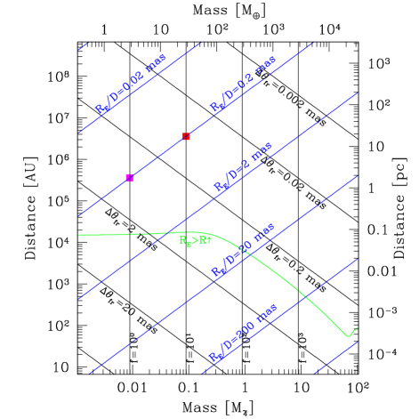
Figure 1: The values of $f$, $R_{E}$ and $\Delta\theta_{\mathrm{fr}}$ as a function of the mass of the substellar object and its distance for $\lambda=10^{1.5}{\rm cm}$ or $\nu\approx 1{\rm GHz}$. The value of $f$ scales as $\nu$ or $\lambda^{-1}$. The slanted black lines follow the locus of constant fringe angular size in the limit of large $f$. They move upwards in proportional to the wavelength. The green curve $R_{E}>R$ indicates the region within which the Einstein radius is larger than the radius of the object so lensing will dominate over occultation, assuming the equation of state of Chabrier et al. (2009) above the mass of Jupiter and the mass-radius relation defined by Saturn, Uranus and Earth for lower masses. Lines indicating both the angular size of the Einstein radius and the value of $f$ are shown as well.

The region of the solar neighborhood and mass of the intervening substellar object where lensing is important is shown in Fig. 1. In particular above the line $R_{E}>R$ lensing begins to dominate over occultation. For the masses of interest this corresponds to objects farther than about a tenth of a parsec; therefore, beyond a parsec lensing strongly dominates. If the source is a giant in the bulge its angular radius is typically about 20 $\mu$as. More distant sources will appear smaller; however, they would be difficult if not impossible to detect with the SKA. If the lens lies well below the blue line ($R_{E}/D=0.02$ mas) and the source is a bulge giant, then the optical light curve would be similar to that of a point source. If the lens lies above or near the black line ($\pi R_{E}/(fD)=0.02$ mas), the fringes would begin to be washed out due to the finite size of the source; therefore, if a lensing event on a bulge star lacks finite-size effects in the optical and lacks fringes at one-metre, then the lens must lie the wedge well above the black line and well below the blue line. One could look for fringes at lower frequencies to further restrict the properties of the lens; however, the sources might be difficult to detect at such low frequencies (§4).

3.2 Light Curves

More tantalizing than a null result would be the detection of fringes (Fig. 2) or a lack of magnification at the longer wavelength. By comparing the optical light curve (green in Fig 2) to the light curve at lower frequencies one could determine the value of $f$ for the lens at the lower frequency. Even if the fringes are diluted by finite source effects, the diffraction does still cause the light curve to vary. Typically if there are six fringes across the disk of the source (red curve), the difference between the light curve according to geometric optics and the diffractive result is a few percent. For twenty fringes over the stellar disk, the difference is a few parts per thousand. If the source is a bulge giant (with a radius twenty times that of the sun), this would correspond to the uppermost black line labelled “$\Delta\theta_{\mathrm{fr}}=0.002$mas.”

For values of $f<1$ there is typically little magnification. The absence of magnification at a particular wavelength would restrict the lens to have a Schwarzschild radius less than that wavelength — a low mass lens. On the other hand, the detection of some magnification along with fringes would determine the value of $f$ constraining the lens to lie on one of the vertical lines in Fig. 1 and giving the mass of the lens. The distance to the lens would also be constrained by the relative amplitude of the fringing if the angular size of the source is comparable or larger than that of fringes.

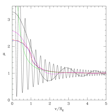
Figure 2: The values of the magnification $\mu$ as a function of the distance between the source and the centre of the lens in units of the Einstein radius, $v/R_{E}$. The result for $f=1$ is the slowly varying sinusoidal curve and $f=10$ is the more rapidly varying one. The magnification from geometric optics is plotted in green. Notice for $f=10$ there are about three peaks over a length of one Einstein radius. The other colours assume that the angular radius of the source equals the Einstein radius. Blue is the geometric optics result, red is for $f=10$ and magenta is $f=1$ (see also the squares in Fig. 1).

For wavelengths less than a metre and lens masses greater than a tenth of a Jupiter mass, the value of $f$ is much greater than unity. In this limit the fringe pattern approaches a simple cosine dependence (Eq. 6) as can be seen in Fig. 3. In the limit of large $f$ the peak magnification is simply $\pi f$ while in the geometric optics limit the magnification diverges as the source lens and observer become aligned.

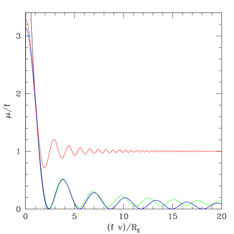
Figure 3: Red, green and blue curves trace the magnification as a function of distance from the centre of the lens for $f=1,10$ and 100 respectively. The magnification according to Bessel function in Eq. 6 is indistinguishable from the blue curve ($f=100$). The black curve gives the approximation using the cosine in Eq. 6.

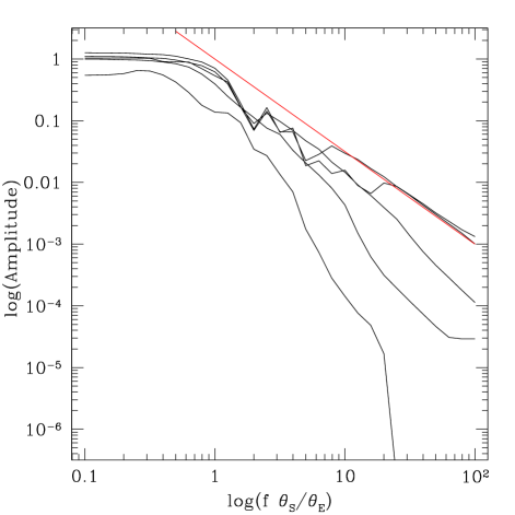
Figure 4: The typical amplitude of the diffractive microlensing signal over the range $0.2<v/R_{E}<3$ as a function of the ratio of angular size of the source $\theta_{s}=R_{s}/D_{s}$ to that of the fringes. The number of fringes across the source is given approximately by $2/\pi f\theta_{S}/\theta_{E}$. The red line shows the relation where the amplitude equals $(f\theta_{s}/\theta_{E})^{-1.5}$. From top to bottom $f=100,10^{1.5},10,10^{1/2}$ and 1.

According to Fig. 4, the relative amplitude of the variation is approximately equal to $(f\theta_{s}/\theta_{E})^{-1.5}$ for large values of $f$ and $(f\theta_{s}/\theta_{E})$. The amplitude of the power-law relation depends on what portion of the light curve is examined; however, the exponent comes simply from the integral of a sinusoid (Eq. 6) over the circular source

$$\int_{-1}^{1}dx\sqrt{1-x^{2}}\cos\left(kx+a\right)=\frac{\pi\cos a}{k}J_{1}(k)\propto k^{-3/2}$$ (8)

where $k\propto f\theta_{S}/\theta_{E}$. The final proportionality holds for values of $k$ much greater than one. The derivation of this expression clearly only makes sense if $f\gg 1$ and $\theta_{S}\ll\theta_{E}$

More generally the relative amplitude of the variation can be taken to be a power law to give

$$\Delta f_{\nu} \approx A\left(f\frac{\theta_{s}}{\theta_{E}}\right)^{-\alpha}f_{\nu}=Af_{\nu,d}^{\alpha/2}f_{\nu}^{(2-\alpha)/2}$$ (9)

$$= f_{\nu,d}^{3/4}f_{\nu}^{1/4}$$ (10)

for $f_{\nu}>f_{\nu,d}$ and $f\gg 1$ and where

$$f_{\nu,d}=\frac{kT_{b}}{2\pi R_{E}^{2}}=0.4\mathrm{nJy}\frac{T_{b}}{1000~{}\mathrm{K}}\frac{M_{\oplus}}{M_{d}}\frac{1~{}\mathrm{pc}}{D_{d}}$$ (11)

and $T_{b}$ is the brightness temperature of the source and $f_{\nu}$ is the flux density of the source.

3.3 Detection

For simplicity it can be assumed that the diffractive microlensing event introduces a sinusoidal variation on the radio emission from the source. Although this variation is not strictly sinusoidal, it is approximately sinusoidal in the limit of large $f$. The Square Kilometre Array is planned to have a sensitivity of $10^{4}\mathrm{m}^{2}\mathrm{K}^{-1}$ (Schilizzi et al., 2007) or a noise level of $0.27$ Jy per Nyquist sample. Using the spectral properties of Gaussian noise, one could detect a sinusoidal variation in the flux of the source down to an amplitude of

$$\Delta f_{\nu}=20.~{}\mathrm{nJy}\left[1+0.21\ln(N_{\mathrm{Trials}})\right]^{1/2}\left(\frac{B}{10\mathrm{GHz}}\frac{t}{2\mathrm{days}}\right)^{-1/2}$$ (12)

with at most a one-percent false-positive rate. The quantity $B$ is the bandwidth of the observation and $t$ is its duration that is set by the length of the typical microlensing event as well as observing efficiencies. In order to use a large bandwidth to decrease the noise level, one must divide the large bandwidth up finely because the flux varies at different rates at different observing frequencies. Without dividing the bandwidth the variation will be smeared out. This is similar in spirit to the process of dedispersion in pulsar searches where the pulse phase depends on the observing frequency (Manchester & Taylor, 1977). Here the frequency of the variation itself depends on the observing frequency.

This detection threshold does not include noise associated with the source, either internal or external (such as scintillation). Typically because the sources are not much brighter than the detection threshold, the relative variation due to microlensing is large, so the other sources of noise proportional to the strength of the source are assumed to lie below the detection threshold.

4 The Sources

Although this detection limit is quite faint, it is unusual for typical microlensing sources to be bright radio sources, so the effect will be difficult to detect. The sources can be divided into essentially two classes. The first are experiencing a microlensing event due an intervening lens detected in the optical. The second are bright compact radio sources that could be lensed by nearby objects serendipitously. Because the Square Kilometre Array in principle can look at all of the sources in a portion of sky all the time, monitoring all of these sources is a possibility only limited by the available computing power.

Because the current slew of radio telescopes are not sensitive enough to detect typical sources for microlensing in the Galactic bulge and the Magellanic clouds, observations of local analogues must provide an estimate of the expected radio spectra of these objects.

4.1 Low-Mass Stars

To survey the types of common radio sources in the bulge, it is natural to focus on local low-mass stars that also happen to be radio sources. Typically isolated low-mass stars do not exhibit strong continuous radio emission. Even at the modest distance of one parsec, the radio emission from the quiet sun is only about one $\mu$Jy (Verschuur & Kellermann, 1988). At one kiloparsec this is down to one pJy, well below the detection threshold of even the SKA. Fortunately, evolved low-mass stars exhibit much greater quiescent radio emission than the sun; these objects will be the focus.

4.1.1 Giants

Arcturus ($\alpha$ Böotis) at 11.25 pc is one of the closest giant stars to Earth (Perryman et al., 1997). Drake & Linsky (1986) presented observations of this star at 2 cm and 6 cm with flux densities of 0.68 mJy and 0.28 mJy respectively. At both wavelengths the emission is well characterised by a brightness temperature of about $1.3\times 10^{4}$ K — the source is larger at longer wavelengths. At a distance of 1 kpc the flux density would be

$$f_{\nu}\approx 24.~{}\mathrm{nJy}\nu_{\mathrm{GHz}}^{0.8}\left(\frac{1~{}\mathrm{kpc}}{D_{s}}\right)^{2}.$$ (13)

using the spectral index found by Drake & Linsky (1986). This yields an expected amplitude variation of

$$\Delta f_{\nu}\approx 12.~{}\mathrm{nJy}\left(\frac{M_{\oplus}}{M_{d}}\frac{1~{}\mathrm{pc}}{D_{d}}\right)^{3/4}\left(\frac{1~{}\mathrm{kpc}}{D_{s}}\right)^{1/2}.$$ (14)

at 10 GHz.

4.1.2 Asymptotic Giants

The nearby variable M7-giant star Mira (o Ceti) provides an exemplar for the rarer asymptotic giant stars observed by OGLE in the bulge of our galaxy. Reid & Menten (1997) find that the radio emission of Mira is well fit by a blackbody emission with $S_{\nu}\approx 6\nu_{\mathrm{GHz}}^{2}\mu\mathrm{Jy}$, and Hipparcos found its distance to be about 110 pc (Perryman et al., 1997), yielding a diameter of about 8 AU. The signal of a diffractive lensing event on a Mira-like star ($T_{b}=1500$ K) at 10 GHz is given by

$$\Delta f_{\nu}\approx 6.3~{}\mathrm{nJy}\left(\frac{M_{\oplus}}{M_{d}}\frac{1~{}\mathrm{pc}}{D_{d}}\right)^{3/4}\left(\frac{1~{}\mathrm{kpc}}{D_{s}}\right)^{1/2}.$$ (15)

Although an AGB star is typically more luminous that a giant both in the optical and the radio, flux only plays a subordinate role in the expected diffractive microlensing variation, the significantly lower brightness temperature of the AGB stars in the radio reduces the expected signal.

4.2 Supergiants

The M2-supergiant Betelgeuse ($\alpha$ Orionis) provides an exemplar for the red supergiant stars observed by OGLE in the Magellanic clouds, assuming a distance of 48 kpc to the Large Magellanic Cloud. Newell & Hjellming (1982) find that the spectrum of Betelgeuse is well characterised by $S_{\nu}\approx 240\nu_{\mathrm{GHz}}^{1.32}\mu\mathrm{Jy}$, and Harper et al. (2008) give a distance of 197 pc to this object. Lim et al. (1998) found that the photosphere at a wavelength of 7 mm subtends an ellipse about 95 mas by 80 mas. The signal of a diffractive lensing event on a Betelgeuse-like star ($T_{b}=2500$ K) at 10 GHz is given by

$$\Delta f_{\nu}\approx 3.0~{}\mathrm{nJy}\left(\frac{M_{\oplus}}{M_{d}}\frac{1~{}\mathrm{pc}}{D_{d}}\right)^{3/4}\left(\frac{48~{}\mathrm{kpc}}{D_{s}}\right)^{1/2}.$$ (16)

The increased luminosity of the supergiant Betelgeuse is offset by its larger size and flatter spectrum.

Drake & Linsky (1989) found that the B8-supergiant Rigel ($\beta$ Orionis) has a flux density of 270$\mu$Jy at 6.3 cm and a brightness temperature of about 15000 K. They argue for a spectrum $f_{\nu}\propto\nu^{0.6}$ yielding the signal of a diffractive lensing event on a Rigel-like star at 10 GHz of

$$\Delta f_{\nu}\approx 6.8~{}\mathrm{nJy}\left(\frac{M_{\oplus}}{M_{d}}\frac{1~{}\mathrm{pc}}{D_{d}}\right)^{3/4}\left(\frac{48~{}\mathrm{kpc}}{D_{s}}\right)^{1/2}.$$ (17)

assuming that the distance to Rigel is 237 pc (Perryman et al., 1997). Even bluer stars yield even higher variable flux densities. Using the O4-supergiant HD 190429 as an exemplar yields

$$\Delta f_{\nu}\approx 37.~{}\mathrm{nJy}\left(\frac{M_{\oplus}}{M_{d}}\frac{1~{}\mathrm{pc}}{D_{d}}\right)^{3/4}\left(\frac{48~{}\mathrm{kpc}}{D_{s}}\right)^{1/2}$$ (18)

so a nearby diffractive lensing event would be detectable against an early supergiant in the Large Magellanic Cloud (LMC) or Small Magellanic Cloud (SMC).

For all of these estimates the only source of noise included is at the receiver. The radio emission of giants and supergiants may be sufficiently noisy to increase the detection limits outlined in § 3.3.

4.3 Radio-loud Quasars

Nearby radio-loud quasars typically have brightness temperatures of about $10^{11}$ K and flux densities of about 1 Jy, much brighter than typical stars; however, they, of course, are much rarer and it is less likely that nearby substellar objects will cause lensing events. The assumption that the quasar lies at a distance of about 1 Gpc and the lens lies in the solar neighbourhood

$$f_{\nu,d}=\frac{kT_{b}}{2\pi R_{E}^{2}}=40\mathrm{mJy}\frac{T_{b}}{10^{11}~{}\mathrm{K}}\frac{M_{\oplus}}{M_{d}}\frac{1~{}\mathrm{pc}}{D_{d}}.$$ (19)

Any quasar with $f_{\nu}<f_{\nu,d}$ would exhibit large oscillations in its flux during a diffractive microlensing event; whereas brighter sources would exhibit variations of

$$\Delta f_{\nu}=90.\mathrm{mJy}\left(\frac{T_{b}}{10^{11}~{}\mathrm{K}}\frac{M_{\oplus}}{M_{d}}\frac{1~{}\mathrm{pc}}{D_{d}}\right)^{3/4}\left(\frac{f_{\nu}}{1~{}\mathrm{Jy}}\right)^{1/4}.$$ (20)

Although lensing events with quasars are likely to be rare, with the SKA it may be possible to monitor a sample of bright quasars continually and provide constraints on the number of freely floating planets. On the other hand radio emission of quasars is inherently noisy. This might make detecting the diffractive lensing events difficult or produce false detections. Either of these possibilities merit further study.

4.4 OGLE-II Sources

To estimate the number of sources that could be detected in the radio with the SKA and whose oscillatory flux could be detected, a detection threshold of 10 nJy is chosen. The radio flux density from each of the OGLE-II sources also has to be modelled. The relationship between bolometric correction, $V-I$-colour and effective temperature given in Sparke & Gallagher (2007) provides a estimate of the angular size of the stellar photosphere as a function of $V-I$ and $V$. This relationship depends only weakly on the luminosity class of the stars. The radio flux is assumed to be proportional to the angular size of the photosphere and normalised to the values for Arcturus in Eq. 13 at 10 GHz. These curves are shown in red in Fig. 5 and the corresponding values of $\Delta f_{\nu}$ are shown in blue. The normalisation to Arcturus is given in purple and the value of $f_{\nu,d}$ in cyan.

The reddening in the OGLE-II fields is extensive (Sumi, 2004). The minimum and maximum mean reddenings are given by the blue arrows, and they are nearly parallel with the curves of constant radio flux, so the individual stars do not need to be dereddened to get a rough estimate of their radio fluxes. The OGLE-II photometry database (Szymanski, 2005; Udalski et al., 1997) contains about 21000 OGLE-II bulge sources with $\Delta f_{\nu}>10$ nJy at 10 GHz and 85000 OGLE-II bulge sources with $f_{\nu}>10$ nJy at 10 GHz. This should be compared with the number of red clump, red giants and red supergiants that Sumi et al. (2006) used to detect microlensing events (1,084,267 stars); therefore, about eight percent of microlensing events may be detectable in the radio. Furthermore, if the lens is about an Earth mass within a few parsecs about two percent of the sources would yield a detectable oscillatory signal. Only a handful of stars in the OGLE-II LMC and SMC fields are sufficiently bright to yield a detectable radio source.

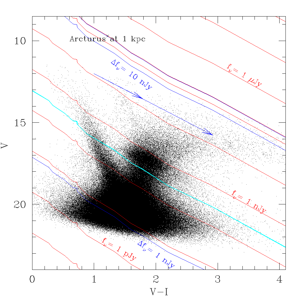
Figure 5: The estimate of the radio flux density (red) and amplitude of its oscillation (blue) at 10 GHz for stars in the bulge field 1 of the OGLE-II survey (Szymanski, 2005; Udalski et al., 1997). The fluxes are normalaized using the values for Arcturus at 1 kpc Eqs. 13 and 14 (purple curve). The cyan line denotes the value of $f_{\nu,d}$ (Eq. 11) for $T_{b}=13000$ K. The minimum and maximum mean reddening lines derived from OGLE-II are given by the blue arrows (Sumi, 2004).

Of course all of these estimates assume that the sources only emit essentially thermal radiation from near their optical photospheres. In fact some fraction of the stars in the bulge and Magellanic Clouds will be radio loud, but it will take an instrument with a sensitivity rivalling that of the SKA to determine their number; therefore, these estimates provide a moderately conservative lower limit on the number of expected radio sources in the bulge at this flux density.

The optical depth of a particular set of objects to microlensing is proportional to their mass fraction; the area subtended by the Einstein radius of a particular lens is proportional to its mass, so the total area (and therefore optical depth) of a particular group of the lenses is proportional to their total mass. A simple model is to assume that the density of lenses is constant out to some maximal distance, yielding

$$\tau=\frac{2\pi G}{c^{2}}\rho l^{2}=2.3\times 10^{-8}\left(\frac{l_{\mathrm{max}}}{1~{}\mathrm{kpc}}\right)^{2}\frac{\rho_{\mathrm{lens}}}{\rho_{\mathrm{Hipparcos}}}$$ (21)

where the dynamical mass estimate of the local disk ($0.076{\rm M}_{\odot}\mathrm{pc}^{-3}$) from Hipparcos (Creze et al., 1998) provides an upper limit on the mass density of lenses within the Galactic disk. This is of course a rough model of the lensing optical depth as the density of lenses will change along the line of sight in a realistic Galactic model, and some substellar lenses may lie in the halo. However, only a rough estimate is warranted because the density of substellar objects is unknown and it is unlikely to exceed about one-tenth of the stellar density (Chabrier, 2002). This yields a rough upper limit on the lensing optical depth of $\tau\lesssim 2\times 10^{-9}$. If one monitors the $10^{5}$ stars in the OGLE-II survey that are also detectable with the SKA and assumes an event duration of one day, one would expect to find a single diffractive lensing event during which the source and lens align to within one Einstein radius about 14 years. Searching for lensing events among fainter stars will not improve this situation because they would probably not be detectable with the SKA. However, monitoring a larger field of stars (going wide rather than deep) would increase this rate proportionally to the number of bright stars.

5 Conclusions

The Square-Kilometer Array will offer an unprecedented view of the radio sky both in terms of sensitivity and cadence. These two factors make it a potential instrument to search for microlensing in the radio. In the spectral range of the SKA diffraction is important to understand the microlensing by objects less massive than Jupiter. The diffractive elements of the microlensing event offer a model-independent way to estimate the mass of the lens that can only otherwise be inferred through statistical arguments.

As Peterson & Falk (1991) argue quasars are among best the best candidates for finding this effect. However, bright quasars are relatively rare and possibly their inherent noise is sufficient to mask the lensing-induced oscillations. This letter argues that the oscillations are also detectable for blue supergiants in the LMC and nearly detectable for giants in the bulge. However, the likelihood of a lensing event against the former is very small due to the small number of blue supergiants in the Magellanic clouds. Because of the relative rarity of blue supergiants and quasars on the sky, most promising potential sources for diffractive microlensing are giant stars — although even in this case the rate is quite low using the OGLE-II stars.

Of course all of these estimates assume that the radio emission of giant and supergiant stars is similar to the few local detections. In fact understanding the emission from these stars is one of the objectives of the SKA, and if the emission turns out to be stronger the prospects are even better. Even if the oscillations are not observable, searching for the frequency at which the magnification deviates from the geometric optics result would indicate that $f\sim 1$ and also provide a mass estimate. Such a measurement would simply require that the source be detectable with the SKA, a much less stringent requirement than detecting the oscillations themselves.

Although this paper has outlined the potential benefits of observing lensing events in the radio that derive from the diffractive aspects of microlensing, there are several important reasons to follow up lensing events in the radio even if the diffractive effects are unlikely to be observable. In particular the lenses themselves may be radio sources — this would yield an estimate of the lens proper motion as well as its identity. If the source can be detected in the radio, observations in the radio could probe the astrometric signature of the lensing event, providing additional constraints.

Several potential substellar lensing events have already been observed, and over the next decades many more will be found as the monitoring campaigns become more sensitive and extensive. Following these events up in the radio with an instrument like the SKA may provide important constraints on their properties and the constituents of the solar neighbourhood.

References

- Chabrier (2002) Chabrier G., 2002, Astrophys. J, 567, 304
- Chabrier et al. (2009) Chabrier G., Baraffe I., Leconte J., Gallardo J., Barman T., 2009, in E. Stempels ed., American Institute of Physics Conference Series Vol. 1094 of American Institute of Physics Conference Series, The mass-radius relationship from solar-type stars to terrestrial planets: a review. pp 102–111
- Creze et al. (1998) Creze M., Chereul E., Bienayme O., Pichon C., 1998, Astron. Astrophys., 329, 920
- Deguchi & Watson (1986a) Deguchi S., Watson W. D., 1986a, Astrophysical Journal, 307, 30
- Deguchi & Watson (1986b) Deguchi S., Watson W. D., 1986b, Physical Review D (Particles and Fields), 34, 1708
- Di Stefano (2009) Di Stefano R., 2009, Astrophysical Journal, submitted, arxiv:0912.1611
- Drake & Linsky (1986) Drake S. A., Linsky J. L., 1986, Astron. J, 91, 602
- Drake & Linsky (1989) Drake S. A., Linsky J. L., 1989, Astron. J, 98, 1831
- Gradshteyn & Ryzhik (1994) Gradshteyn I. S., Ryzhik I. M., 1994, Table of Integrals, Series, and Products, fifth edn. Academic Press
- Harper et al. (2008) Harper G. M., Brown A., Guinan E. F., 2008, Astron. J, 135, 1430
- Heyl (2010) Heyl J., 2010, Monthly Notices, 402, L39
- Lim et al. (1998) Lim J., Carilli C. L., White S. M., Beasley A. J., Marson R. G., 1998, Nature, 392, 575
- Manchester & Taylor (1977) Manchester R. N., Taylor J. H., 1977, Pulsars.. W. H. Freeman, San Francisco
- Newell & Hjellming (1982) Newell R. T., Hjellming R. M., 1982, Astrophys. J Lett, 263, L85
- Perryman et al. (1997) Perryman M. A. C., et al., 1997, Astron. Astrophys., 323, L49
- Peterson & Falk (1991) Peterson J. B., Falk T., 1991, Astrophys. J Lett, 374, L5
- Reid & Menten (1997) Reid M. J., Menten K. M., 1997, Astrophys. J, 476, 327
- Schilizzi et al. (2007) Schilizzi R. T., et al., 2007, Technical report, Preliminary Specifications for the Square Kilometre Array. Square Kilometre Array
- Schneider et al. (1992) Schneider P., Ehlers J., Falco E. E., 1992, Gravitational Lenses. Springer, Berlin
- Sparke & Gallagher (2007) Sparke L. S., Gallagher III J. S., 2007, Galaxies in the Universe: An Introduction. Cambridge University Press
- Sumi (2004) Sumi T., 2004, Monthly Notices, 349, 193
- Sumi et al. (2006) Sumi T., Woźniak P. R., Udalski A., Szymański M., Kubiak M., Pietrzyński G., Soszyński I., Żebruń K., Szewczyk O., Wyrzykowski Ł., Paczyński B., 2006, Astrophys. J, 636, 240
- Szymanski (2005) Szymanski M. K., 2005, Acta Astron., 55, 43
- Udalski et al. (1997) Udalski A., Kubiak M., Szymanski M., 1997, Acta Astron., 47, 319
- Verschuur & Kellermann (1988) Verschuur G. L., Kellermann K. I., eds, 1988, Galactic and Extragalactic Radio Astronomy, second edn. Springer-Verlag, New York