Consistency of $\Lambda$CDM with Geometric and Dynamical Probes

Abstract

The $\Lambda$CDM cosmological model assumes the existence of a small cosmological constant in order to explain the observed accelerating cosmic expansion. Despite the dramatic improvement of the quality of cosmological data during the last decade it remains the simplest model that fits remarkably well (almost) all cosmological observations. In this talk I review the increasingly successful fits provided by $\Lambda$CDM on recent geometric probe data of the cosmic expansion. I also briefly discuss some emerging shortcomings of the model in attempting to fit specific classes of data (eg cosmic velocity dipole flows and cluster halo profiles). Finally, I summarize recent results on the theoretically predicted matter overdensity ($\delta_{m}=\frac{\delta\rho_{m}}{\rho_{m}}$) evolution (a dynamical probe of the cosmic expansion), emphasizing its scale and gauge dependence on large cosmological scales in the context of general relativity. A new scale dependent parametrization which describes accurately the growth rate of perturbations even on scales larger than $100h^{-1}Mpc$ is shown to be a straightforward generalization of the well known scale independent parametrization $f(a)=\Omega_{m}(a)^{\gamma}$ valid on smaller cosmological scales.

1 Introduction

Converging geometrical [1, 2, 3, 4, 5, 6] and dynamical [7, 8, 9, 10, 11] cosmological observations indicate that the universe has entered a phase of accelerating expansion. This expansion could be driven either by the negative pressure of a homogeneous dark energy component [12] or by a modified gravitational force which is repulsive on large cosmological scales. Alternatively it could simply be due to an unusually large underdensity (void) on scales of about 1Gpc which induces an apparent isotropic accelerating expansion to observers located approximately at the center of the void [13]. All of the above three classes of models attempting to explain the observed accelerating expansion suffer from fine tuning problems which are reflected in the unexpected values of the parameters required to fit the cosmological expansion data. For example dark energy originating from an evolving scalar field requires a scalar field mass of order $10^{-42}GeV$ which is several orders of magnitude smaller from expectations based on particle physics theories. Similarly, models assuming the existence of large voids require fine tuning of the location of the earth based observer within about $20Mpc$ from the $1Gpc$ large void while the formation of such a large void is also very unlikely in the context of standard cosmology [13].

The simplest and most successful model consistent with (almost) all cosmological data is the $\Lambda$CDM model[14]. This model is based on a modified version of Einstein’s equations of the form

$$R_{\mu\nu}-\frac{1}{2}Rg_{\mu\nu}+\Lambda g_{\mu\nu}=8\pi GT_{\mu\nu}$$ (1)

where $\Lambda$ is a new free parameter, the cosmological constant. When the new term $\Lambda g_{\mu\nu}$ is placed on the left hand side (lhs) of equation (1) it is interpreted as a modification of the gravitational law corresponding to an effective Newton potential [14]

$$V(r)=-\frac{GM}{r}-\Lambda r^{2}$$ (2)

where $-\Lambda r^{2}$ corresponds to a new repulsive gravitational term. When the new term $\Lambda g_{\mu\nu}$ is placed on the right hand side (rhs) of equation (1) it is interpreted as a new contribution to the energy momentum tensor $T_{\mu\nu}$ corresponding to dark energy with constant density $\rho_{\Lambda}=\frac{\Lambda}{8\pi G}$ and constant negative pressure $p_{\Lambda}=-\rho_{\Lambda}$.

Consistency with cosmological data requires a fine tuned value for $\rho_{\Lambda}$

$$\rho_{\Lambda}^{(obs)}\simeq(10^{-12}GeV)^{4}\simeq 2\times 10^{-10}erg/cm^{3}$$ (3)

A physically motivated origin of the cosmological constant could be the energy of the quantum field vacuum which is predicted to have a constant diverging energy density and negative pressure. Under the assumption of a proper cutoff the quantum vacuum can be made finite and play the role of a cosmological constant. A natural scale for this cutoff is the Planck scale leading to a vacuum density

$$\rho_{\Lambda}^{(Pl)}\simeq(10^{18}GeV)^{4}\simeq 2\times 10^{110}erg/cm^{3}$$ (4)

which is 120 orders of magnitude larger than the observed value.

Despite of the unnaturally small value of the observed $\rho_{\Lambda}^{(obs)}$ when compared to the anticipated value $\rho_{\Lambda}^{(Pl)}$ in the context of vacuum energy, the cosmological constant of equation (1) has some unique physically motivated features. In particular the lhs of equation (1) is the most general second rank tensor which is

• local

• coordinate covariant

• divergenceless (needed for energy momentum conservation)

• symmetric

An additional important attractive feature of $\Lambda$CDM is simplicity. It is the only model based on General Relativity (GR) which (assuming flatness) involves a single free parameter ($\Omega_{\Lambda}\equiv\frac{\rho_{\Lambda}}{\rho_{c}}=1-\Omega_{0{\rm m}}$ where $\rho_{c}$ is the present day critical density required for a flat universe) and its predicted expansion rate $H(z)=\frac{\dot{a}}{a}(z)$ as a function of redshift $z$

$$H(z)^{2}=H_{0}^{2}\left[\Omega_{0{\rm m}}(1+z)^{3}+(1-\Omega_{0{\rm m}})\right]$$ (5)

is currently consistent with all cosmological expansion probes (geometric and dynamical). It is therefore clear that the identification of potential conflicts of $\Lambda$CDM with cosmological data is a prerequisite before seriously considering alternative more complicated models unless such models are free from any type of fine tuning. Unfortunately no such model is currently known.

Cosmological observations testing the $\Lambda$CDM model include two classes of probes

• Geometric probes which measure directly the cosmic metric (eg Type Ia supernovae as standard candles or Cosmic Microwave Background (CMB) spectrum peaks and Baryon Acoustic Oscillations (BAO) which use the last scattering horizon scale as a standard ruler)

• Dynamical probes which measure simultaneously the cosmic metric and the gravitational law on cosmological scales. The main dynamical probe is the evolution of linear dark matter cosmological perturbations $\delta_{m}(k,z)=\frac{\delta\rho_{m}}{\rho_{m}}(k,z)$ as a function of scale and redshift. This evolution can be probed either directly through weak lensing observations[15] or indirectly though the large scale power spectrum of luminus matter at various redshifts [16].

Geometric probes provide currently the most accurate information about the cosmic expansion rate $H(z)$ as a function of redshift. In the first part of this brief review (section 2) I discuss the following three basic questions

1. What is the figure of merit [17] (constraining power) of various recent Type Ia supernovae (SnIa) datasets and how does it compare with the corresponding figure of standard ruler (CMB+BAO) geometric probe data?

2. What is the consistency level of various geometric probe datasets with $\Lambda$CDM?

3. What is the level of consistency between standard candle SnIa datasets and standard ruler CMB+BAO geometric probes?

A few cosmological observations which appear to be in some tension [18] with the predictions of $\Lambda$CDM will also be discussed in section 2. The most interesting of these observations appears to be the observed dipole velocity flows on scales larger than $50h^{-1}Mpc$ which appear to be a factor of about four larger than the $\Lambda$CDM model predictions assuming normalization of the matter fluctuation power spectrum using the WMAP5 CMB data[19, 20, 21]. Other puzzling observations include the high redshift brightness of SnIa [22], the cluster halo profiles [23, 24] and the emptiness of voids [25, 26, 27].

The theoretically predicted linear evolution of cosmological perturbations $\delta_{m}(k,z)$ as a function of redshift and scale, depends sensitively on both the expansion rate and the gravitational law on cosmological scales. This dual sensitivity makes the linear evolution of density perturbations a particularly useful dynamical cosmological probe. Even though current observational constraints on $\delta_{m}(k,z)$ are not as powerful as geometric constraints on $H(z)$ this is expected to change dramatically in the next decade [28].

The time evolution of matter density perturbations $\delta_{m}(k,t)$ is described by the well known equation (see eg [8])

$${\ddot{\delta}_{m}}+2H{\dot{\delta}_{m}}-4\pi G\rho_{m}f(k,t)\delta_{m}=0$$ (6)

where in the context of general relativity $f(k,t)=1$ and $\delta_{m}(k,t)=\delta_{m}(t)$ becomes independent of the scale $k$. In fact, this scale independence of $\delta_{m}$ is occasionally considered to be a signature of validity of general relativity[29]. However, the derivation of equation (18) is based on two important assumptions whose validity is questionable on scales $(\buildrel>\over{\sim}200h^{-1}Mpc)$. These assumptions are the following:

1. The scale of the perturbation $\delta_{m}$ is significantly smaller than the Hubble scale at all times during the perturbation evolution.

2. The choice of gauge plays a minor role in the form of the evolution equation for $\delta_{m}$.

An important question discussed in the second part of this review (section 3) is the following: What is the level of validity of these assumptions on large cosmological scales? It can be shown that the validity of both assumptions breaks down rapidly as the scale increases beyond $200h^{-1}Mpc$.

2 $\Lambda$CDM confronts Recent Geometric Cosmological Data

A useful way to test the $\Lambda$CDM model is to consider a generalized parametrization of the dark energy equation of state which includes $\Lambda$CDM as a special parameter case and find the likelihood of the parameters corresponding to $\Lambda$CDM in this context. A commonly used such parametrization is the Chevallier-Polarski, Linder (CPL)[30, 31] ansatz

$$w=w_{0}+w_{1}(1-a)=w_{0}+w_{1}\frac{z}{1+z}$$ (7)

which reduces to $\Lambda$CDM for $(w_{0},w_{1})=(-1,0)$. In this section, I show the ranking of the six latest Type Ia supernova (SnIa) datasets (see Table 1) (Constitution (C), Union (U), ESSENCE (Davis) (E), Gold06 (G), SNLS 1yr (S) and SDSS-II (D)) in the context of the CPL parametrization (7) according to their Figure of Merit (FoM)[17], their consistency with the cosmological constant ($\Lambda$CDM) and their consistency with standard rulers (Cosmic Microwave Background (CMB) and Baryon Acoustic Oscillations (BAO)). The datasets considered are shown in Table (1) along with some useful features such as the redshift range or the subsets of each set[32].

Assuming a CPL parametrization for $w(z)$ (equation (7)) it is possible to apply the maximum likelihood method separately for standard rulers (CMB+BAO) and standard candles (SnIa) assuming flatness. The corresponding late time form of $H(z)$ for the CPL parametrization is

$$H^{2}(z) = H_{0}^{2}[\Omega_{\rm 0m}(1+z)^{3}+$$ (8)

$$+ (1-\Omega_{\rm 0m})(1+z)^{3(1+w_{0}+w_{1})}e^{\frac{-3w_{1}z}{(1+z)}}]\,.$$

Table 1: The datasets used in the present analysis. See respective references for details on the sources of the SnIa data points.

Dataset	Date Released	Redshift Range	# of SnIa	Filtered subsets included
SNLS1 [33]	2005	$0.015\leq z\leq 1.01$	115	SNLS [33], LR [34]
Gold06 [35]	2006	$0.024\leq z\leq 1.76$	182	SNLS1 [33], HST [35], SCP [1], HZSST [2]
ESSENCE [36],[37]	2007	$0.016\leq z\leq 1.76$	192	SNLS1 [33], HST [35], ESSENCE[36],[37]
Union [38]	2008	$0.015\leq z\leq 1.55$	307	Gold06 [35], ESSENCE[36], [37]
Constitution [3]	2009	$0.015\leq z\leq 1.55$	397	Union [38], CfA3[3]
SDSS [39]	2009	$0.022\leq z\leq 1.55$	288	Nearby [40], SDSS-II [39], ESSENCE [36], SNLS [33], HST [35]

The SnIa observations use light curve fitters[40] to provide the apparent magnitude $m(z)$ of the supernovae at peak brightness. The resulting apparent magnitude $m(z)$ is related to the dimensionless luminosity distance $D_{L}(z)$ through [41, 32]

$$m_{th}(z)={\bar{M}}(M,H_{0})+5log_{10}(D_{L}(z))\,,$$ (9)

where

$$D_{L}(z)=(1+z)\int_{0}^{z}dz^{\prime}\frac{H_{0}}{H(z^{\prime};\Omega,w_{0},w_{1})}$$ (10)

is the Hubble free luminosity distance ($H_{0}d_{L}$), and ${\bar{M}}$ is the magnitude zero point offset and depends on the absolute magnitude $M$ and on the present Hubble parameter $H_{0}$ as

$${\bar{M}} = M+5log_{10}(\frac{H_{0}^{-1}}{Mpc})+25=$$ (11)

$$= M-5log_{10}h+42.38.$$

The parameter $M$ is the absolute magnitude which is assumed to be constant after proper corrections (using light curve fitters) have been implemented in $m(z)$.

The theoretical model parameters are determined by using the maximum likelihood method ie by minimizing the quantity

$$\chi^{2}_{SnIa}(\Omega,w_{0},w_{1})=\sum_{i=1}^{N}\frac{(\mu_{obs}(z_{i})-\mu_{th}(z_{i}))^{2}}{\sigma_{\mu\;i}^{2}}$$ (12)

where $N$ is the number of SnIa of the dataset and $\sigma_{\mu\;i}^{2}$ are the errors due to flux uncertainties, intrinsic dispersion of SnIa absolute magnitude and peculiar velocity dispersion. These errors are assumed to be Gaussian and uncorrelated. The theoretical distance modulus is defined as

$$\mu_{th}(z_{i})\equiv m_{th}(z_{i})-M=5log_{10}(D_{L}(z))+\mu_{0}\,,$$ (13)

where

$$\mu_{0}=42.38-5log_{10}h\,,$$ (14)

The steps followed for the usual minimization of (12) in terms of its parameters are described in detail in [32, 41, 16, 42].

In the context of constraints from standard rulers from CMB spectrum peaks [41, 32], the maximum likelihood method is used and the datapoints $(R,l_{a},100\Omega_{b}h^{2})$ of Ref. [4] (WMAP5) where $R$, $l_{a}$ are two shift parameters [41]. In the case of BAO, the maximum likelihood method is also applied [41] using the datapoints of Ref. [43] (SDSS5). For comparison, the more recent data of Ref. [5] (SDSS7) have also been considered with only minor differences in the results (slightly reduced consistency with $\Lambda$CDM in the context of the CPL parametrization but no change in the ranking sequences).

The Figure of Merit (FoM) is a useful measure of the effectiveness of a set of data in constraining cosmological parameters. In the case of two parameters (as for the CPL parametrization) it is defined as the reciprocal area of the $95.4\%$ contour (see Fig. 2), in parameter space $(w_{0},w_{1})$ [17]. Clearly, the larger the FoM the more effective the dataset in constraining the parameters $(w_{0},w_{1})$. Fig. 1 shows the FoM in terms of the number of the SnIa data for the datasets of Table 1. Clearly, the FoM is an increasing function of the number of SnIa in the datasets. An exception to this rule is the ESSENCE dataset which has a slightly smaller FoM compared to the Gold06 dataset even though it has a larger number of SnIa. A possible origin of this effect is the fact that the FoM does not depend only on the total number of SnIa of the dataset but mainly on the number of SnIa at low and high redshifts (the redshift space distribution of the ESSENCE data includes more data at intermediate redshifts than the Gold06 dataset).

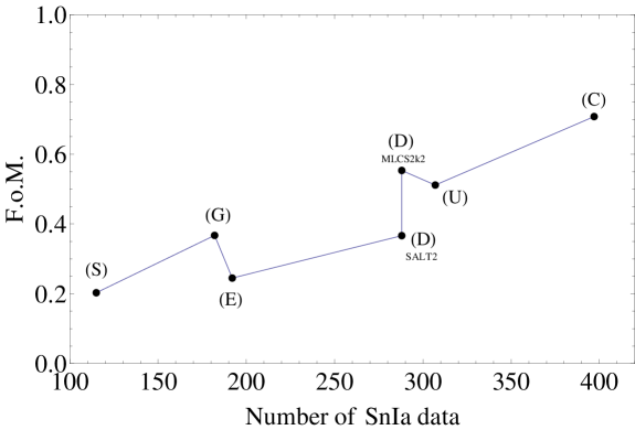
Figure 1: The Figure of Merit (FoM) in terms of the number of the SnIa data for $\Omega_{0{\rm m}}=0.28$ using the CPL parametrization.

In order to study the consistency of the various SnIa datasets with the cosmological constant and the standard rulers we consider the distance in units of $\sigma$ ($\sigma$-distance $d_{\sigma}$) of the best fit point to a model with parameters $(w_{0},w_{1})$, where this reference point can be either $\Lambda$CDM or some other reference point, (see Fig. 2). The $\sigma$-distance can be found by converting $\Delta\chi^{2}=\chi^{2}_{(w_{0},w_{1})}-\chi^{2}_{min}$ to $d_{\sigma}$, i.e. solving [44]

$$1-\Gamma(1,\Delta\chi^{2}/2)/\Gamma(1)={\rm Erf}(d_{\sigma}/\sqrt{2})$$ (15)

for $d_{\sigma}$ ($\sigma$-distance), where $\Delta\chi^{2}$ is the $\chi^{2}$ difference between the best-fit and the reference point ($w_{0},w_{1})$ (eg $\Lambda$CDM) and ${\rm Erf}()$ is the error function. The right hand side of Eq. (15) comes from integrating $\int_{-n\sigma}^{~{}n\sigma}\frac{1}{\sigma\sqrt{2\pi}}~{}e^{-\frac{x^{2}}{2\sigma^{2}}}dx$, where $n$ is the desired number of $\sigma$s, while the left hand side corresponds to the Cumulative Distribution Function (CDF) of a $\chi^{2}$ distribution[44] with two degrees of freedom. Note that Eq. (15) is only valid for the two parameters $(w_{0},w_{1})$ and should be generalized accordingly for more parameters [44]. In the special case of $n=1$ or $n=2$ we obtain the well known results $\Delta\chi_{1\sigma}=2.30$ and $\Delta\chi_{2\sigma}=6.18$ valid for two parameter parametrizations [44].

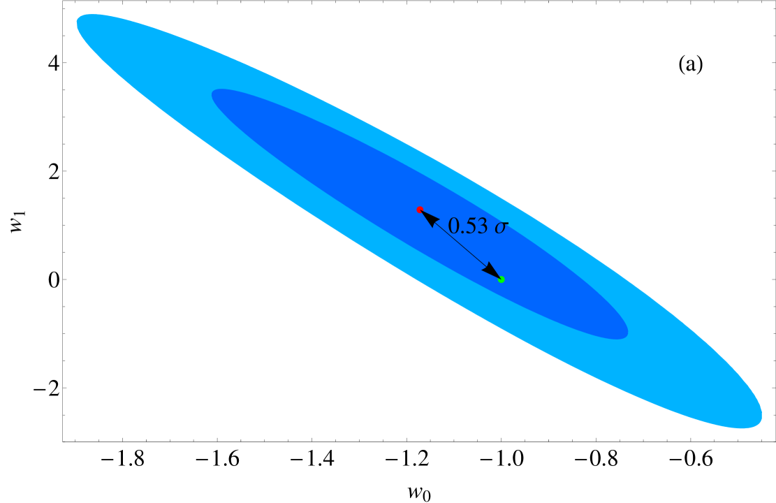
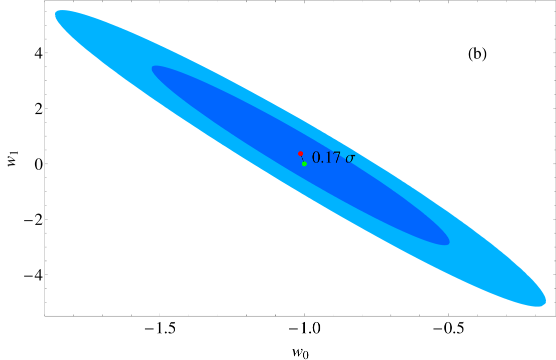
Figure 2: The $68.3\%(1\sigma)-95.4\%$ ($2\sigma$) $\chi^{2}$ confidence contours in the $w_{0}-w_{1}$ plane based on parametrization (8) for the ESSENCE (left) and SNLS1 datasets (right) for $\Omega_{0{\rm m}}=0.24$. The arrows indicate the $\sigma$-distance of $\Lambda$CDM (green points: $(w_{0},w_{1})=(-1,0)$) to the best fit points (red points).

Even though the $\sigma$-distance is not a commonly used statistic it is quite useful because it can directly give information about probability of a given region in parameter space. The integer values of sigma distance ($1\sigma$ and $2\sigma$) are commonly used to draw the corresponding contours in parameter space. The extension of this statistic to non-integer values is used to find the specific contours that go through particular reference points of parameter space and thus estimate quantitatively the consistency of these points. The advantage of using the $\sigma$-distance instead of $\Delta\chi^{2}$ is the fact that the $\sigma$-distance takes into account the number of parameters of the parameterizations and can therefore be directly translated into probability for each point in parameter space. This is not possible for $\Delta\chi^{2}$ because it does not include information about the number of parameters of the parameterizations considered.

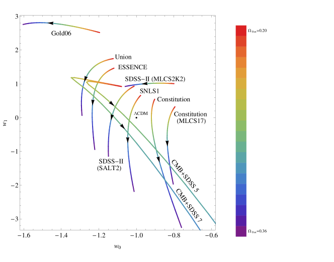
Figure 3: Trajectories of the best fit points $(w_{0},w_{1})$ obtained for each of the datasets of Table 1 and also for the standard ruler CMB-BAO (WMAP5+SDSS5 and WMAP5+SDSS7) data as $\Omega_{0{\rm m}}$ varies in the range $\Omega_{0{\rm m}}\in[0.2,0.36]$. The arrows in the best fit lines indicate the direction of growing $\Omega_{0{\rm m}}$. Note that for the SDSS5 data the standard ruler best fit parameters stretch out to $(w_{0},w_{1})\simeq(2,-30)$ for $\Omega_{0{\rm m}}\simeq 0.36$, whereas for the SDSS7 data $(w_{0},w_{1})\simeq(0.90,-20)$.

It is straightforward to apply the likelihood method to find the trajectory of the best fit point $(w_{0},w_{1})$ in parameter space as $\Omega_{0{\rm m}}$ varies in the range $\Omega_{0{\rm m}}\in[0.2,0.36]$. These trajectories obtained for each of the datasets of Table 1 and also for the standard ruler CMB-BAO (WMAP5+SDSS5, WMAP5+SDSS7) data are shown in Fig. 3. These trajectories can not be used to directly rank the datasets according to their consistency with any given reference point in parameter space (e.g. $\Lambda$CDM) because they contain no information about the $68.3\%$ ($1\sigma$) contours. However, they provide useful hints for the trend of the best fit parameters as $\Omega_{0{\rm m}}$ varies. For example, such a trend is the increase of the best fit value of the slope $w_{1}$ as the prior of $\Omega_{0{\rm m}}$ decreases towards the value $0.2$ or that the best fit value of $w_{0}$ remains less than $-1$ for all datasets except of the Constitution compilation.

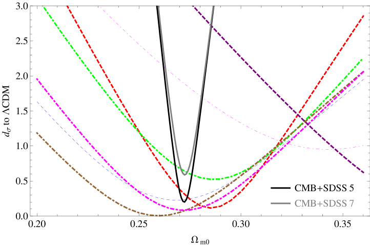
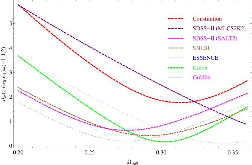
Figure 4: a: $\sigma$-distances $d_{\sigma i}(\Omega_{0{\rm m}};-1,0)$ off the $\Lambda$CDM point (reference point) from the best fit of each dataset in Table 1. Notice that the best fit of each dataset, except for the Gold06 and the SDSS-II (MLCS2k2), are minimized at similar values of $\Omega_{0{\rm m}}$. The $\sigma$-distance $d_{\sigma}(\Omega_{0{\rm m}};-1,0)$ between the standard ruler best fits and $\Lambda$CDM are also shown as a function of $\Omega_{0{\rm m}}$ (black and grey solid lines). b: Similar to (a) for the dynamical dark energy reference point $(w_{0},w_{1})=(-1.4,2)$. Notice that the $\sigma$-distances $d_{\sigma i}(\Omega_{0{\rm m}};-1.4,2)$ are minimized at more widely separated values of $\Omega_{0{\rm m}}$.

The ranking sequence of the datasets of Table 1 with respect to any reference point in parameter space can be studied quantitatively using the $\sigma$-distance statistic discussed above. In order to test the sensitivity of the ranking sequence of datasets with respect to the choice of consistency reference point $(w_{0},w_{1})$ we consider two such reference points: $(w_{0},w_{1})=(-1,0)$ ($\Lambda$CDM) and $(w_{0},w_{1})=(-1.4,2)$ which corresponds to dynamical dark energy with a $w(z)$ that crosses the line $w=-1$. It should be noted that there is nothing special about the parameter point (-1.4,2). We have selected it as a representative of a wide region in parameter space (upper left from $\Lambda$CDM) which corresponds to dynamical dark energy crossing the phantom divide line $w=-1$. Any other point in the same parameter region would lead to similar results and the same ranking of datasets. This particular parameter region is interesting because it is spanned by the best fit trajectories and it also mildly favored by the Gold06 dataset (see Fig. 3).

The resulting $d_{\sigma}(\Omega_{0{\rm m}})$ for each dataset of Table 1 are shown in Figs. 4 in the range $\Omega_{0{\rm m}}\in[0.2,0.36]$.

Table 2: Minimum $\sigma$-distance $d_{\sigma}^{min}(\Omega_{0{\rm m}}^{min};-1,0)$ from the best fit point for each of the datasets to the $\Lambda$CDM point. Also listed are the corresponding values of $\Omega_{0{\rm m}}$, and the best fit parameters $(w_{0},w_{1})$ (see also Fig. 4a). The SDSS-II (MLCS2K2) data showed no minimum of $d_{\sigma}$ with respect to $\Omega_{0{\rm m}}$ in the range $\Omega_{0{\rm m}}\in[0.2,0.36]$. We thus have simply displayed the lowest value of $d_{\sigma}$ in the corresponding range of $\Omega_{0{\rm m}}$.

Dataset	$d_{\sigma}^{min}$	$\Omega_{0m}^{min}$	$w_{0}$	$w_{1}$
SNLS1	0.004	0.260	-1.03	0.16
SDSS-II (SALT2)	0.084	0.270	-1.09	0.51
Constitution	0.114	0.285	-0.91	-0.54
ESSENCE	0.227	0.270	-1.20	1.04
Union	0.525	0.285	-1.25	1.40
SDSS-II (MLCS2K2)	0.623	0.360	-1.06	0.93
Gold06	0.950	0.345	-1.56	2.80
CMB+BAO (SDSS5)	0.200	0.272	-1.15	0.51
CMB+BAO (SDSS7)	0.588	0.272	-1.30	0.97

Clearly, there are values of $\Omega_{0{\rm m}}$ that minimize the $\sigma$-distance $d_{\sigma}(\Omega_{0{\rm m}})$ between the best fit of each dataset and the reference point. These values of $\Omega_{0{\rm m}}$ maximize the consistency of the datasets with the given reference point in this range of $\Omega_{0{\rm m}}$. The minima $\sigma$-distances $d_{\sigma}(\Omega_{0{\rm m}})$ for each dataset, corresponding to maximum consistency with $\Lambda$CDM along with the corresponding values of $\Omega_{0{\rm m}}$ are shown (properly ranked) in Table 2. The corresponding results for the reference point $(w_{0},w_{1})=(-1.4,2)$ are shown in Table 3.

Table 3: The minimum $\sigma$-distances $d_{\sigma}^{min}$ to the reference point $(w_{0},w_{1})=(-1.4,2)$, the values of $\Omega_{0{\rm m}}$ at which the minimum distance is attained, and the best fit parameters $(w_{0},w_{1})$ at $\Omega_{0{\rm m}}^{min}$ are displayed for each dataset (see also Fig. 4b). We omit the rows corresponding to CMB+BAO data as the resulting $\sigma$-distance is always $\gg 1$ due to the dominance of the dark energy at early times. The SDSS-II (MLCS2K2) data showed no minimum of $d_{\sigma}$ with respect to $\Omega_{0{\rm m}}$ in the range $\Omega_{0{\rm m}}\in[0.2,0.36]$. We thus have simply displayed the lowest value of $d_{\sigma}$ in the corresponding range of $\Omega_{0{\rm m}}$.

Dataset	$d_{\sigma}^{min}$	$\Omega_{0m}^{min}$	$w_{0}$	$w_{1}$
Gold06	0.11	0.345	-1.56	2.80
Union	0.17	0.300	-1.26	1.25
ESSENCE	0.19	0.275	-1.21	0.99
SNLS1	0.42	0.290	-1.04	-0.26
SDSS-II (SALT2)	0.63	0.275	-1.10	0.46
SDSS-II (MLCS2K2)	0.87	0.360	-1.06	0.93
Constitution	1.77	0.315	-0.88	-1.32

The following comments can be made with respect to the results shown in Figs. 4 and in the corresponding Tables 2, 3.

1. The consistency with $\Lambda$CDM of all datasets, except Gold06 and SDSS-II when using the MLCS2K2 method, is maximized in a narrow range of $\Omega_{0{\rm m}}\in[0.26,0.29]$ which also includes the value of $\Omega_{0{\rm m}}$ favored by standard rulers. On the other hand, the consistency with the dynamical dark energy point $(w_{0},w_{1})=(-1.4,2)$ is maximized over a wider range of $\Omega_{0{\rm m}}$ ($\Omega_{0{\rm m}}\in[0.27,0.35]$) thus decreasing the consistency among the datasets in the context of dynamical dark energy.

2. The ranking sequence changes dramatically when the consistency with the dynamical dark energy is considered as a reference point instead of $\Lambda$CDM (Table 3). Essentially the ranking is reversed! Thus, the choice of the consistency reference point plays an important role in determining the ranking sequence of the datasets (see also Fig. 4).

3. The SDSS-II dataset obtained with the MLCS2k2 fitter has some peculiar features compared to other datasets. In particular it favors particularly high values of $\Omega_{0{\rm m}}$ ($\Omega_{0{\rm m}}\simeq 0.4$) while for $\Omega_{0{\rm m}}<0.3$ its consistency with $\Lambda$CDM is significantly reduced to a level of $3\sigma$ or larger ($d_{\sigma}>3$). In addition, the trajectory of its best fit parameter point as $\Omega_{0{\rm m}}$ varies is perpendicular to the corresponding trajectory of most other datasets (see Fig. 4).

It is straightforward to apply the $\sigma$-distance statistic to rank the SnIa datasets according to their consistency with standard ruler CMB-BAO data. We simply use as a consistency reference point the best fit point $(w_{0},w_{1})^{SR}$ for standard rulers obtained as described in section 2 using the WMAP5+SDSS5 data. In this case, the location of the reference point $(w_{0},w_{1})^{SR}$ in parameter space depends on $\Omega_{0{\rm m}}$ but this does not complicate the analysis. The $\sigma$-distance between the reference point $(w_{0},w_{1})^{SR}$ and the best fit of each dataset is shown in Fig. 5 as a function of $\Omega_{0{\rm m}}$ for the datasets of Table 1. These distances are minimized for values of $\Omega_{0{\rm m}}$ that are different for each dataset but they are all in the narrow range $\Omega_{0{\rm m}}\in[0.27,0.3]$.

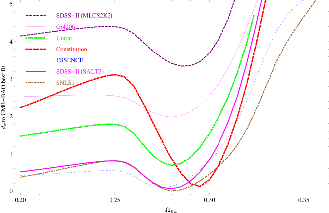
Figure 5: $\sigma$-distance $d_{\sigma i}(\Omega_{0{\rm m}};(w_{0},w_{1})^{SR})$ between the reference point $(w_{0},w_{1})^{SR}$ of standard rulers (using the WMAP5+SDSS5 data) and the best fit of each dataset as a function of $\Omega_{0{\rm m}}$ for the datasets of Table 1. Using the SDSS7 data, the minimum distances are found in the range $\Omega_{0{\rm m}}\in[0.29,0.31]$.

These minimum distances along with the corresponding value of $\Omega_{0{\rm m}}$ are shown in Table 4 for each dataset (properly ranked according to consistency with standard rulers). Notice that the ranking sequence for the consistency with standard rulers is practically identical to the ranking sequence of the consistency with $\Lambda$CDM (Table 2) but differs from the ranking sequence of the consistency with dynamical dark energy (Table 3). This is an interesting feature of the data in favor of $\Lambda$CDM.

Table 4: Consistency with standard rulers. Minimum $\sigma$-distance $d_{\sigma i}^{min}(\Omega_{0{\rm m}};(w_{0},w_{1})^{SR})$ between best fit parameters for each dataset, $(w_{0},w_{1})$, and best fit for standard rulers, $(w_{0},w_{1})^{SR}$. $d_{\sigma i}^{min}(\Omega_{0{\rm m}};(w_{0},w_{1})^{SR})$ is minimized at $\Omega_{0{\rm m}}^{min}$ (see Fig. 5).

Dataset	$d_{\sigma}^{min}$	$\Omega_{0m}^{min}$	$w_{0}$	$w_{1}$	$w_{0}^{SR}$	$w_{1}^{SR}$
SNLS1	0.003	0.280	-1.04	-0.10	-1.07	0.08
SDSS-II (SALT2)	0.058	0.280	-1.11	0.40	-1.07	0.08
ESSENCE	0.087	0.275	-1.21	0.99	-1.12	0.38
Constitution	0.121	0.295	-0.90	-0.76	-0.84	-1.28
Union	0.681	0.280	-1.24	1.44	-1.07	0.08
Gold06	1.976	0.280	-1.38	2.75	-1.07	0.08
SDSS-II(MLCS2K2)	3.342	0.285	-0.92	1.02	-1.00	-0.28

It is therefore clear that the $\Lambda$CDM cosmological model is a well defined, simple and predictive model which is consistent with the majority of current cosmological observations. Despite of these successes there are specific cosmological observations which differ from the predictions of $\Lambda$CDM at a level of $2\sigma$ or higher. The observations conflicting the WMAP5 normalized $\Lambda$CDM model at a level of $2\sigma$ or larger include the following [18]:

• Large Scale Velocity Flows ($\Lambda$CDM predicts significantly smaller amplitude and scale of flows than what observations indicate)[19, 20, 21]. The probability of consistency with $\Lambda$CDM is about $1\%$.

• Brightness of Type Ia Supernovae (SnIa) at High Redshift $z$ ($\Lambda$CDM predicts fainter SnIa at High $z$)[22]. The probability of consistency with $\Lambda$CDM is about $3-5\%$ for the Union and Gold06 datasets.

• Emptiness of Voids ($\Lambda$CDM predicts more dwarf or irregular galaxies in voids than observed)[25, 26, 27].

• Profiles of Cluster Haloes ($\Lambda$CDM predicts shallow low concentration and density profiles in contrast to observations which indicate denser high concentration cluster haloes) [23, 24].

• Profiles of Galaxy Haloes[45] ($\Lambda$CDM predicts halo mass profiles with cuspy cores and low outer density while lensing and dynamical observations indicate a central core of constant density and a flattish high dark mass density outer profile),

• Sizable Population of Disk Galaxies[46] ($\Lambda$CDM predicts a smaller fraction of disk galaxies due to recent mergers expected to disrupt cold rotationally supported disks).

Even though some of the puzzles discussed here may be resolved by more complete observations or astrophysical effects, the possible requirement of more fundamental modifications of the $\Lambda$CDM model remains valid.

3 Dynamical Probes: The Growth Function

3.1 Growth of Perturbations in General Relativity: Beyond the sub-Hubble Approximation

As discussed in the introduction, the evolution of the matter overdensity $\delta_{m}(k,a)$ (the growth function) consists a useful probe of both the expansion rate and the gravitational law on large scales. The standard parametrization of the linear growth function $\delta_{m}(k,a)$ is scale independent and is obtained by introducing a growth index $\gamma$ defined through the growth rate $f(a)$ by

$$f_{0}(a)\equiv\frac{d\ln\delta_{m}}{d\ln a}=\Omega_{m}(a)^{\gamma}$$ (16)

where $a=\frac{1}{1+z}$ is the scale factor and

$$\Omega_{m}(a)\equiv\frac{H_{0}^{2}\Omega_{0{\rm m}}a^{-3}}{H(a)^{2}}$$ (17)

is the ratio of the matter density to the critical density when the universe has scale-factor $a$ where $H_{0}$ is Hubble constant and $\Omega_{0m}$ is ratio of mass density to critical density. This parametrization [47] provides an excellent fit to the evolution equation for $\delta_{m}(a)$ in general relativity and in the small scale (sub-Hubble) approximation

$${\ddot{\delta}}_{m}+2H{\dot{\delta}}_{m}-4\pi G\rho_{m}\delta_{m}=0$$ (18)

where an overdot denotes the derivative with respect to time and $\rho_{m}$ is the matter density. Changing variables from $t$ to $\ln a$ we obtain the evolution equation for the growth factor $f$ as

$$f^{\prime}+f^{2}+f(\frac{\dot{H}}{H^{2}}+2)=\frac{3}{2}\Omega_{m}$$ (19)

where ${}^{\prime}=d/dlna$. For dark energy models in a flat universe with a slowly varying equation of state $w(a)\equiv\frac{p(a)}{\rho(a)}=w_{0}$, the solution of eq. (19) is well approximated by eq. (16) with [47]

$$\gamma=\frac{3(w_{0}-1)}{6w_{0}-5}$$ (20)

which reduces to $\gamma=\frac{6}{11}$ for the $\Lambda$CDM case ($w_{0}=-1$). It is therefore clear that the observational determination of the growth index $\gamma$ can be used to test $\Lambda$CDM [9]. It has been shown [11] that even in the context of dynamical dark energy models consistent with Type Ia supernovae (SnIa) observations the parameter $\gamma$ does not vary by more than $5\%$ from its $\Lambda$CDM value. However, in the context of modified gravity models $\gamma$ can vary by as much as $30\%$ (e.g. for the DGP model[48] $\gamma_{DGP}\simeq 0.68$ [11]) while scale dependence is also usually introduced[49, 50, 10].

Current observational constraints on $\gamma$ are based on redshift distortions of galaxy power spectra [51], the rms mass fluctuation $\sigma_{8}(z)$ inferred from galaxy and $Ly-\alpha$ surveys at various redshifts [52, 53], weak lensing statistics [54], baryon acoustic oscillations [55], X-ray luminous galaxy clusters [56], Integrated Sachs-Wolfe (ISW) effect [57] etc. Unfortunately, the currently available data are limited in number and accuracy and come mainly from the first two categories. They involve significant error bars and non-trivial assumptions that hinder a reliable determination of $\gamma$. Thus, the current constraints on $\gamma$ are fairly weak [9] and are expressed as

$$\gamma=0.674^{+0.195}_{-0.169}$$ (21)

This however is expected to change in the next few years when more detailed weak lensing surveys [15] are anticipated to narrow significantly the above range[28].

A crucial assumption made in the derivation of eq. (18) in the context of general relativistic metric perturbations is the assumption that the scale of the perturbations is significantly smaller than the Hubble scale [47]. This assumption however does not lead to a good approximation on scales larger than about $100h^{-1}Mpc$ [58, 59]. In order to demonstrate this fact consider the perturbed metric of spacetime which takes the form (in the Newtonian gauge):

$$ds^{2}=-(1+2\Phi)dt^{2}+(1-2\Phi)a^{2}\gamma_{ij}dx^{i}dx^{j},$$ (22)

where $\gamma_{ij}$ is the metric of the spatial section and we are ignoring anisotropic stresses. The evolution of density perturbations on all scales is dictated by combining the background equations

$$H^{2} = \frac{8\pi G}{3}(\rho_{m}+\rho_{de})$$ (23)

$${\dot{\rho}} = -3H(\rho+p)$$ (24)

(assuming a flat universe with only pressureless dark matter and (non-clustering) dark energy) with the perturbed linear order Einstein equations in the Newtonian gauge [60] ($\rho_{m}$ and $\rho_{de}$ are the matter and dark energy densities respectively while $p=w\rho$ is the pressure). The resulting (anisotropic stress-free) equations are of the form

$$\ddot{\Phi} = -4H\dot{\Phi}+8\pi G\rho_{de}w_{de}\Phi$$ (25)

$$\dot{\delta} = 3\dot{\Phi}+\frac{k^{2}}{a^{2}}v_{f}$$ (26)

$$\dot{v}_{f} = -\Phi$$ (27)

with constraint equations

$$3H(H\Phi+\dot{\Phi})+\frac{k^{2}}{a^{2}}\Phi = -4\pi G\delta\rho_{m}$$ (28)

$$(H\Phi+\dot{\Phi}) = -4\pi G\rho_{m}v_{f}$$ (29)

where $\Phi$ is the Newtonian potential, $v_{f}\equiv-va$ ($v$ is the velocity potential for dark matter). Clearly, equations (25)-(27) involve a scale $k$ dependence in contrast to the small scale approximate equation (18) which is scale independent.

The derivation of equation (18) in the context of general relativity is made using the sub-Hubble approximation. The linear matter overdensity $\delta\rho_{m}$ may be expressed [60] in terms of the gravitational potential $\Phi$ and the background variables as follows:

$$-4\pi G\delta\rho_{m}=\frac{k^{2}}{a^{2}}\Phi+3H^{2}\Phi+3H\dot{\Phi}$$ (30)

In the sub-Hubble (small scale) approximation ($\frac{k^{2}}{a^{2}}\gg H^{2}$) equation (30) takes the form

$$-4\pi G\delta\rho_{m}=\frac{k^{2}}{a^{2}}\Phi$$ (31)

where a slowly varying gravitational potential $\Phi$ has also been assumed.

The general relativistic equations (25)-(29) lead to the following equation for the matter overdensity $\delta_{m}$

$${\ddot{\delta}_{m}}+2H{\dot{\delta}_{m}}+\frac{k^{2}}{a^{2}}\Phi=0$$ (32)

which also expresses the conservation of the perturbed energy momentum tensor for matter. Using the sub-Hubble approximation (31) we obtain the scale independent approximate equation (18). On the other hand, if we avoid this approximation in equation (30), solve for $\Phi$ (ignoring the time derivative) and substitute in equation (32) we obtain the following scale dependent evolution equation for $\delta_{m}$ [58, 59]:

$${\ddot{\delta}_{m}}+2H{\dot{\delta}_{m}}-\frac{4\pi G\rho_{m}\delta_{m}}{1+\xi(a,k)}=0$$ (33)

where

$$\xi(a,k)=\frac{3a^{2}H(a)^{2}}{k^{2}}$$ (34)

The solution of equation (33) provides a much better approximation to the full linear general relativistic system (25)-(27) up to horizon scales. On scales larger than the horizon even equation (33) breaks down since on these scales, the time derivative of $\Phi$ can not be ignored.

Given the successful approximation of the solution of (33) to the exact linear general relativistic solution, it becomes important to construct a scale dependent parametrization that is analogous to (16) and solves (approximately) (33) for all scales $k$. In order to construct such a parametrization we focus on the matter dominated era when most of the growth occurs and express $\xi(a,k)$ as

$$\xi(a,k)=\frac{3H_{0}^{2}\Omega_{0{\rm m}}}{ak^{2}}$$ (35)

Equation (33) may be expressed in terms of the growth factor $f=\frac{d\ln\delta_{m}}{d\ln a}$ in the form

$$f^{\prime}+f^{2}+\left(2-\frac{3}{2}\Omega_{m}(a)\right)f=\frac{3}{2}\frac{\Omega_{m}(a)}{1+\xi(a,k)}$$ (36)

where ${}^{\prime}\equiv\frac{d}{d\ln a}$, and we have assumed $\Lambda$CDM for $H(a)$.

For sub-Hubble scales $\xi(k,a)\rightarrow 0$ and equation (36) reduces to (19) whose solution is well approximated by (16) with $\gamma=\frac{6}{11}$. It is straightforward to show using an expansion method [59] that the parametrization

$$f(k,a)=\frac{f_{0}(a)}{1+\xi(k,a)}=\frac{\Omega_{m}(a)^{\gamma}}{1+\frac{3H_{0}^{2}\Omega_{0{\rm m}}}{ak^{2}}}$$ (37)

is an approximate solution of equation (36) and provides a good approximation to the solution of the general relativistic system (25)-(27) up to horizon scales.

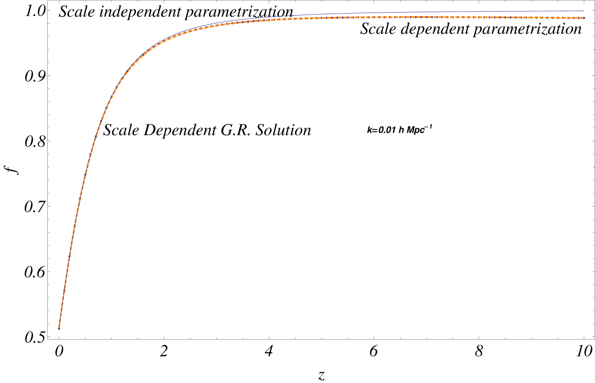
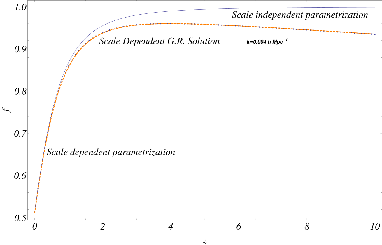
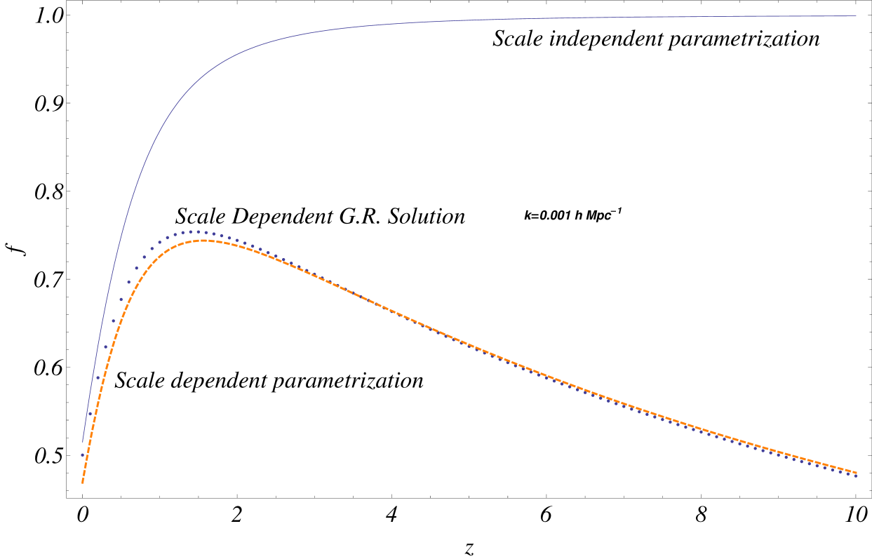
Figure 6: a: The growth rate $f$ obtained from the solution of the general relativistic system ($k=0.01h^{-1}Mpc$, $\Omega_{0{\rm m}}=0.3$, $\Lambda$CDM , dotted line) compared with the scale independent parametrization (continuous line) and the corresponding generalized scale dependent parametrization (thick dashed line) b: Similar to a. for $k=0.004h^{-1}Mpc$. c: Similar to a. for $k=0.001h^{-1}Mpc$.

The accuracy of the parameterization (37) is demonstrated in Fig. 6 where we compare the form of the scale dependent parametrization Eq. (37) with the general relativistic numerical solution and with the standard parametrization for three different scales. It is clear that up to approximately the Hubble scale $(k\simeq 0.001hMpc^{-1})$ the scale dependent parametrization (37) is accurate at a level better than $5\%$ at least up a to redshift $z=10$. It can be shown that this parametrization is also a good approximation to the growth rate not only in the $\Lambda$CDM model but also in the case of dynamically evolving dark energy. Thus the parametrization described by equation (37) approximates very well the full linear general relativistic solution up to horizon scales and differs significantly from the standard parametrization on scales larger than about $100h^{-1}Mpc$. Its use may play an important role when comparing cosmological structure data on large scales with theoretical model predictions.

As shown in Fig. 6 the range of scales where the standard scale independent parametrization (16) starts breaking down involves scales larger than $100h^{-1}Mpc$ ($k<0.01hMpc^{-1}$). This scale is much smaller than the present Hubble scale which is about $3000h^{-1}Mpc$. Therefore, the sub-Hubble approximation breaks down at much smaller scales than the anticipated Hubble scale. This is due to the fact that at early times during the matter era when most growth occurs, the comoving Hubble scale is significantly smaller compared to its present value. In fact, at recombination it is close to $200h^{-1}Mpc$. Therefore, scales that remain at the sub-Hubble level during the whole time when the growth of matter perturbations take place are only scales below $200h^{-1}Mpc$.

The generalized Poisson equation (30) in the Newtonian gauge may be solved for the slowly varying $\Phi$ leading to a generalized gravitational potential in Fourier space of the form

$$\Phi^{GR}(k)=\frac{\Phi^{Poisson}(k)}{1+\frac{3a^{2}H(a)^{2}}{k^{2}}}$$ (38)

where $\Phi^{Poisson}(k)$ is the usual small scale gravitational potential which emerges as a solution of the usual Poisson equation. In coordinate space the generalized large scale potential potential has a Yukawa form with a Hubble scale cutoff namely

$$\Phi^{GR}(r)=-\frac{GM}{ar}e^{-\sqrt{3}Har}$$ (39)

It is this general relativistic potential that should be compared with corresponding modified gravity potentials on scales comparable to the Hubble scale.

In a modified gravity theory the Poisson equation on large scales is modified for two reasons: First due to the modified gravitational law and second due to the Hubble scale effects that are present also in the case of general relativity as discussed above. The result is a Poisson equation of the form

$$\frac{k^{2}}{a^{2}}\Phi=-4\pi G{\rho}_{m}\delta_{m}(k,a)f(k,a)$$ (40)

where the scale dependent function $f(k,a)$ incorporates the scale dependence due to both Hubble scale effects and scale dependence due to modification of the gravitational law. This function is to be compared with the scale dependence due to pure Hubble scale effects $f_{GR}(k,a)=\frac{1}{1+\xi(a,k)}$ present in general relativity. Therefore a signature of modified gravity would not be a scale dependence of the evolution of matter density perturbations as claimed occasionally in the literature[29], but a deviation from the scale dependence predicted on large scale in the context of general relativity.

3.2 Gauge Dependence

The scale dependence of the matter density growth rate obtained above was based on calculations made in the Newtonian gauge. This is a physically important gauge because it corresponds to a time slicing of isotropic expansion. Nevertheless since the matter density perturbation $\delta_{m}(k,t)$ is a gauge dependent quantity, it is important to clarify to what extend do the results of section 3.1 persist in a gauge different from the Newtonian gauge.

Another important gauge is the synchronous gauge which corresponds to a time slicing obtained by the matter local rest frame everywhere in space (the free falling observer frame). The synchronous gauge is generally considered to be the most efficient reference system for doing calculations. It is used in many modern cosmology codes for calculating the evolution of cosmological perturbations (eg CMBFAST [61]). The line element of the perturbed spacetime in the synchronous gauge is given by

$$ds^{2}=a^{2}(\tau)(-d\tau^{2}+(\delta_{ij}+h_{ij})dx^{i}dx^{j})$$ (41)

where $\tau$ is the conformal time. It is straightforward to derive the growth equation for $\delta_{m}\equiv\delta\rho_{m}/\rho_{m}$ in a matter dominated universe in the synchronous gauge to obtain [60, 58]

$$\ddot{\delta}^{SG}_{m}+2H\dot{\delta}^{SG}_{m}-4\pi\rho_{m}G\delta^{SG}_{m}=0$$ (42)

This growth equation is exact in the synchronous gauge in the case of matter domination and involves no scale dependence as in the case of equation (33) of the Newtonian gauge. This scale independence is an artifact of the particular time slicing of the synchronous gauge which is a good approximation on small scales but is unable to capture the horizon scale effects modifying the growth function on large scales.

Nevertheless equations (33) and (42) clearly agree on small scales where $\xi\rightarrow 0$. Therefore, for larger scales ($k<0.01hMpc$) the question that arises is the following: What is the proper gauge to use when comparing with observations? This question was recently addressed in Ref. [62] where a gauge invariant observable replacement was obtained for $\delta_{m}$. This observable $\delta_{obs}(k,t)$ involves the matter density perturbation $\delta_{m}(k,t)$ corrected for redshift distortions due to peculiar velocities and gravitational potential. It also includes volume and position corrections. The final expression however is complicated and makes the theoretical predictions based on it not easy to implement and manipulate.

Alternatively, the gauge-invariant (GI) approach to the cosmological perturbations evolution, pioneered by Bardeen[63] may be used to identify observables (e.g., Refs.[64, 65]). The most general form of the line element for a spatially flat background and scalar metric perturbations can be written as [65]

$$ds^{2}=a^{2}\{(1+2\Phi)d\tau^{2}-2B_{\mid i}dx^{i}d\tau-[\delta_{ij}-2(\Psi\delta_{ij}-E_{\mid_{ij}})]dx^{i}dx^{j}~{}\},$$ (43)

where $a$ and $\tau$ are the conformal cosmic expansion scale factor and the conformal cosmic time; “_∣” denotes the background three-dimensional covariant derivative. The corresponding perturbed energy-momentum tensor $T^{\mu}_{\nu}$ has the form

$$T^{0}_{~{}0} = \rho_{m}(1+\delta_{m})~{},$$

$$T_{0}^{~{}i} = \rho_{m}U_{\mid i}~{},$$

$$T^{0}_{~{}i} = -\rho_{m}(U-B)_{\mid i}~{},$$

$$T^{i}_{~{}j} = -\rho_{m}\Sigma_{\mid ij}~{},$$ (44)

where $\rho_{m}$ is the unperturbed pressureless matter density; $U$ and $\Sigma$ determine velocity perturbation and anisotropic shear perturbation.

A gauge-invariant matter density perturbation may be constructed as [63, 64]

$$\delta_{m}^{GIS}\equiv\delta_{m}+3\frac{\dot{a}}{a}(U-B)~{},$$ (45)

$\delta_{m}^{GIS}$ coincides with the density perturbation $\delta_{m}^{(CTG)}$ in the Comoving Time-orthogonal Gauge ($CTG$, in which $U=B=0$), which denotes the density perturbation relative to the spacelike hypersurface which represents the matter local rest frame everywhere[63]. This quantity also coincides with the density perturbation $\delta_{m}^{SG}$ in the Synchronous Gauge (in which $\Psi=\Phi=B=0$) for the pressureless matter system. In other words, $\delta_{m}^{GIS}$ denotes the density perturbation relative to the observers everywhere comoving with the matter. These free falling observers do not experience the isotropic expanding background of the universe because the peculiar velocity of matter is distinct from the Hubble flow. Thus $\delta_{m}^{SGI}$ has physical significance only for perturbations on scales small compared to the Hubble scale.

An alternative gauge-invariant variable is more closely related to the matter overdensity in the Newtonian gauge. This gauge-invariant perturbation variable is of the form [63, 64, 65],

$$\delta_{m}^{GIN}\equiv\delta_{m}+\frac{\dot{\rho}}{\rho}(B-\dot{E})=\delta_{m}-3\frac{\dot{a}}{a}(B-\dot{E})~{}.$$ (46)

and has important advantages over $\delta_{m}^{GIS}$. $\delta_{m}^{GIN}$ coincides with the density perturbation $\delta_{m}^{NG}$ in the Newtonian Gauge ($NG$), in which $B=E=0$.

In addition to the gauge invariant perturbation variable it is straightforward to construct two gauge-invariant scalar potentials $\phi$ and $\psi$, both of which become the same as the gravitational potential in the Newtonian limit. These are constructed from metric perturbations as follows [65]:

$$\phi\equiv\Phi-\frac{\dot{a}}{a}(B-\dot{E})~{},$$

$$\psi\equiv\Psi+\frac{1}{a}\frac{d}{d\tau}[(B-\dot{E})a]~{}.$$ (47)

The relation between $\delta_{m}^{GIS}$ and the general gravitational potential $\phi$ obeys the Poisson equation[63, 64]:

$$\bigtriangledown^{2}\phi=-k^{2}\phi=4\pi G\rho a^{2}\delta_{m}^{GIS}.$$ (48)

where $k$ is the (comoving) wavenumber of Fourier mode. As discussed above, the Poisson equation is valid only for scales small compared to the Hubble radius $1/H$ while on scales larger than the Hubble scale the growth of matter density perturbations is frozen. Hence, $\delta_{m}^{GIS}$ can not be regarded as the observable matter density perturbation on scales comparable to the Hubble scale. Therefore, the observable density perturbation on both the small-scale and the large-scale modes can not be described directly by $\delta_{m}^{GIS}$ even though it is a gauge-invariant quantity.

Contrary to $\delta_{m}^{GIS}$, the other gauge invariant perturbation $\delta_{m}^{GIN}$ has some important attractive features with respect to observability. These are summarized as follows:

• It reduces to the Newtonian gauge perturbation $\delta_{m}^{NG}$ ie it corresponds to a frame which respects the isotropic expansion of the universe and is therefore more appropriate for description of large scale perturbations. This reduction also simplifies the calculation of this perturbation.

• It drives a scale dependent modification of the Poisson equation for the gauge invariant potential $\phi$. Indeed, the time-time part of the linearized Einstein equation gives [65, 60]

  $$\bigtriangledown^{2}\phi-3\frac{\dot{a}}{a}(\frac{\dot{a}}{a}\psi+\dot{\phi})=-k^{2}\phi-3\frac{\dot{a}}{a}(\frac{\dot{a}}{a}\psi+\dot{\phi})=4\pi G\rho a^{2}\delta_{m}^{GIN}.$$ (49)

  Thus, the anticipated scale dependence on scales comparable to the Hubble scale is picked up by the perturbation $\delta_{m}^{GIN}$.

• It is gauge invariant as anticipated for any observable quantity.

These features make the gauge invariant $\delta_{m}^{GIN}$ and the Newtonian gauge $\delta_{m}^{NG}$ to which it reduces, an attractive choice for making theoretical calculations to obtain the gravitational potential and the matter density perturbation that can be directly compared with observations on large scales. However, these theoretically obtained quantities need to also be corrected for bias, redshift distortions (due to gravitational potential and peculiar velocities), lensing magnification and volume distortion[62].

4 Conclusion

I have reviewed the consistency of recent geometric cosmological data with the $\Lambda$CDM cosmological model. The standard candle SnIa datasets considered in this study are consistent with $\Lambda$CDM and with standard rulers at a level of $95.4\%$ ($2\sigma$) or less for certain prior values of the matter density $\Omega_{0{\rm m}}$ in the range $\Omega_{0{\rm m}}\in[0.25,0.35]$. It is interesting that the ranking sequence based on consistency with $\Lambda$CDM is practically identical with the corresponding ranking based on consistency with standard rulers even though the two criteria are completely independent. Thus, despite the improvement of standard ruler and standard candle data quality during the last decade the consistency of $\Lambda$CDM with data has not decreased despite the fact that $\Lambda$CDM is a simple, specific and well defined model which appears as a measure-zero point in all generalized models. On the contrary its consistency seems to be improving with time as new and more accurate data appear. For example, the Constitution SnIa dataset which is a very recent compilation with a drastic improvement on the crucial nearby SnIa sample, is also one of the most consistent datasets with both $\Lambda$CDM and standard rulers.

Despite of its excellent consistency with both SnIa standard candles and CMB-BAO standard rulers, $\Lambda$CDM has to face potential challenges from other cosmological data [18] (e.g. large scale velocity flows, galaxy and cluster halo profiles, peculiar features of CMB maps etc.) which may lead the quest for the properties of dark energy to interesting surprises in the near future. Such surprises may also come from future standard candle observations or standard ruler CMB experiments (e.g. Planck [66]) which are expected to significantly improve the accuracy of the constraints discussed in the present study.

I have also discussed dynamical probes of the cosmological constant and reviewed a scale dependent parametrization of the growth rate $f=\frac{d\ln\delta_{m}}{d\ln a}$ that is free from the sub-Hubble approximation of the standard parametrization (16). This parametrization described by equation (37) approximates very well the full linear general relativistic solution up to horizon scales and differs significantly from the standard parametrization on scales larger than about $100h^{-1}Mpc$. This parametrization describes well the growth of matter density perturbations on large scales in the Newtonian gauge.

Even though the matter density perturbation is a gauge dependent quantity, the Newtonian gauge has certain advantages that make it particularly useful when making a direct comparison of theoretical predictions with observations. These advantages are summarized as follows:

• The evolution of perturbations in the Newtonian gauge picks up the anticipated scale dependence when the Hubble scale is approached.

• The time slicing of the Newtonian gauge respects the isotropic expansion of the background and therefore it is more appropriate to describe large scale fluctuations. On the other hand, the synchronous gauge corresponds to free falling observers at all points and therefore it is physically relevant on small scales where the two gauges give identical evolution of cosmological perturbations.

• Gauge invariant generalizations of the density fluctuation $\delta_{m}$ and the gravitational potential reduce to the corresponding Newtonian quantities in the Newtonian gauge. This identification with gauge invariant quantities is a prerequisite for the direct observability of the density perturbation and the gravitational potential in the Newtonian gauge

Even though additional corrections need to be made to the theoretically predicted value of the density perturbation evolution along the lines of Ref. [62], it is clear that the Newtonian gauge offers a good starting point for the direct comparison of theoretical predictions of dark energy models with observations.

References

References

- [1] Perlmutter et al. 1999, ApJ, 517, 565; Knop et al. 2003, ApJ, 598, 102;
- [2] Riess et al. 1998 AJ, 116, 1009; Clocchiatti et al. 2003, astro-ph/0310432; Riess et al. 2000, ApJ, 536, 62; Tonry et al. 2003, Astrophys.J.594:1-24,2003.
- [3] M. Hicken et al., Astrophys. J. 700, 1097 (2009) [arXiv:0901.4804 [astro-ph.CO]].
- [4] Komatsu E. et al. 2009 [WMAP Collaboration], Ap.J. Suppl. 180, 330.
- [5] Percival W. J. et al. 2009, arXiv:0907.1660.
- [6] Nesseris S. and Perivolaropoulos L. 2007 JCAP 0701, 018; \nonumSanchez J. C. B., Nesseris S. and Perivolaropoulos L. 2009 JCAP 0911, 029.
- [7] Tegmark M. et al. 2004 [SDSS Collaboration], Phys. Rev. D 69, 103501.
- [8] Bertschinger E. 2006 Ap. J. 648, 797; \nonumNesseris S. and Perivolaropoulos L. 2008 Phys. Rev. D 77, 023504; \nonumDi Porto C. and Amendola L. 2008 Phys. Rev. D 77, 083508;
- [9] S. Nesseris and L. Perivolaropoulos, Phys. Rev. D 77, 023504 (2008) [arXiv:0710.1092 [astro-ph]].
- [10] D. Polarski and R. Gannouji, Phys. Lett. B 660, 439 (2008) [arXiv:0710.1510 [astro-ph]].
- [11] E. V. Linder and R. N. Cahn, Astropart. Phys. 28, 481 (2007) [arXiv:astro-ph/0701317].
- [12] Copeland E. J., Sami M. and Tsujikawa S. 2006 Int. J. Mod. Phys. D 15, 1753.
- [13] Iguchi H., Nakamura T. and Nakao K. 2002 Prog. Theor. Phys. 108, 809;\nonumCaldwell R. R. and Stebbins A. 2008 Phys. Rev. Lett. 100, 191302;\nonumVanderveld R. A., Flanagan E. E. and Wasserman I. 2006 Phys. Rev. D 74, 023506.
- [14] Peebles P.J.E. and Ratra B. 2003 Rev. Mod. Phys. 75, 559;\nonumPadmanabhan T. 2003 Phys. Rept. 380, 235;\nonumCarroll S. M. 2001 Living Rev. Rel. 4, 1; \nonumSahni V 2002 Class. Quant. Grav. 19, 3435.
- [15] L. Fu et al., arXiv:0712.0884 [astro-ph]; O. Dore et al., arXiv:0712.1599 [astro-ph]; D. Munshi, P. Valageas, L. Van Waerbeke and A. Heavens, Phys. Rept. 462, 67 (2008) [arXiv:astro-ph/0612667].
- [16] S. Nesseris and L. Perivolaropoulos 2004 Phys. Rev. D 70, 043531.
- [17] Albrecht A.J. et al. 2006 “Report of the Dark Energy Task Force,” arXiv:astro-ph/0609591; arXiv: 0901.0721.
- [18] L. Perivolaropoulos, arXiv:0811.4684 [astro-ph].
- [19] R. Watkins, H. A. Feldman and M. J. Hudson, arXiv:0809.4041 [astro-ph].
- [20] A. Kashlinsky, F. Atrio-Barandela, D. Kocevski and H. Ebeling, arXiv:0809.3734 [astro-ph].
- [21] H. A. Feldman, R. Watkins and M. J. Hudson, arXiv:0911.5516 [Unknown].
- [22] L. Perivolaropoulos and A. Shafieloo, arXiv:0811.2802 [astro-ph].
- [23] T. Broadhurst, K. Umetsu, E. Medezinski, M. Oguri and Y. Rephaeli, Astrophys. J. 685, L9 (2008) [arXiv:0805.2617 [astro-ph]].
- [24] T. J. Broadhurst, M. Takada, K. Umetsu, X. Kong, N. Arimoto, M. Chiba and T. Futamase, Astrophys. J. 619, L143 (2005) [arXiv:astro-ph/0412192].
- [25] A. Tikhonov and A. Klypin, arXiv:0807.0924 [astro-ph].
- [26] P. J. E. Peebles, Nucl. Phys. Proc. Suppl. 138, 5 (2005) [arXiv:astro-ph/0311435].
- [27] A. A. Klypin, A. V. Kravtsov, O. Valenzuela and F. Prada, Astrophys. J. 522, 82 (1999) [arXiv:astro-ph/9901240].
- [28] Zhan H., Knox L. and Tyson J. A. 2009 ApJ 690, 923; \nonumJoudaki S., Cooray A. and Holz D. E. 2009 Phys. Rev. D 80, 023003;\nonumT. Schrabback et al., arXiv:0911.0053; \nonumA. Cimatti et al., arXiv:0912.0914.
- [29] V. Acquaviva, A. Hajian, D. N. Spergel and S. Das, Phys. Rev. D 78, 043514 (2008) [arXiv:0803.2236 [astro-ph]].
- [30] Chevallier M. and Polarski D. 2001 Int. J. Mod. Phys. D 10, 213.
- [31] Linder E. V. 2003 Phys. Rev. Lett. 90, 091301.
- [32] J. C. B. Sanchez, S. Nesseris and L. Perivolaropoulos 2009 JCAP 0911, 029.
- [33] P. Astier et al. [The SNLS Collaboration] 2006 Astron. Astrophys. 447, 31.
- [34] Hamuy et al. 1996 Ap.J. 112, 2408;\nonumRiess et al. 1999 Ap.J. 117, 707;\nonumJha 2002 (PhD thesis Harvard);\nonumKrisciunas 2001 Ap.J. 122, 1616;\nonumKrisciunas, et al. 2004 Ap.J. 128, 3034;\nonumAltavilla et al 2004 MNRAS, 349, 1344.
- [35] A. G. Riess et al. 2007 Ap. J 659, 98.
- [36] W. M. Wood-Vasey et al. [ESSENCE Collaboration] 2007 Ap. J 666 694.
- [37] T. M. Davis et al. 2007 Ap.J. 666, 716.
- [38] M. Kowalski et al. 2008 Ap. J. 686, 749.
- [39] R. Kessler et al. 2009 arXiv:0908.4274 [astro-ph.CO].
- [40] J. Guy et al. 2005 A&A 443, 781; J. Guy et al., A&A 466, 11 (2007);\nonumS. Jha, A. G. Riess and R. P. Kirshner 2007 Ap.J., 659, 122.
- [41] R. Lazkoz, S. Nesseris and L. Perivolaropoulos 2008 JCAP 0807, 012.
- [42] S. Nesseris and L. Perivolaropoulos 2005 Phys. Rev. D 72, 123519.
- [43] W. J. Percival, S. Cole, D. J. Eisenstein, R. C. Nichol, J. A. Peacock, A. C. Pope and A. S. Szalay 2007 Mon. Not. Roy. Astron. Soc. 381, 1053;\nonumD. Eisenstein et al. 2005 Ap. J. 633, 560.
- [44] W. H. Press et. al. 1994 “Numerical Recipes” Cambridge University Press.
- [45] G. Gentile, C. Tonini and P. Salucci 2007 Astron. Astrophys. 467, 925.
- [46] J. S. Bullock, K. R. Stewart and C. W. Purcell 2008 arXiv:0811.0861.
- [47] L. M. Wang and P. J. Steinhardt 1998 Ap. J. 508, 483.
- [48] C. Deffayet 2001 Phys. Lett. B 502, 199.
- [49] S. Nesseris and L. Perivolaropoulos 2007 JCAP 0701, 018.
- [50] J. P. Uzan 2007 Gen. Rel. Grav. 39, 307.
- [51] E. Hawkins et al. 2003 Mon. Not. Roy. Astron. Soc. 346, 78; \nonumE. V. Linder 2007 arXiv:0709.1113 [astro-ph].
- [52] M. Viel, M. G. Haehnelt and V. Springel 2004 Mon. Not. Roy. Astron. Soc. 354, 684.
- [53] M. Viel and M. G. Haehnelt 2006 Mon. Not. Roy. Astron. Soc. 365, 231.
- [54] N. Kaiser 1998 Ap.J. 498, 26; \nonumL. Amendola, M. Kunz and D. Sapone 2007 arXiv:0704.2421 [astro-ph]; \nonumH. Hoekstra et al. 2006 Ap. J. 647, 116.
- [55] H. J. Seo and D. J. Eisenstein 2003 Ap. J. 598, 720 ;\nonumD. Sapone and L. Amendola 2007 arXiv:0709.2792 [astro-ph].
- [56] A. Mantz, S. W. Allen, H. Ebeling and D. Rapetti 2007 arXiv:0709.4294 [astro-ph].
- [57] M. J.Rees and D. W. Sciama 1968 Nature 217 511;\nonumR. G. Crittenden and N. Turok 1996 Phys. Rev. Lett. 76, 575;\nonumL. Pogosian, P. S. Corasaniti, C. Stephan-Otto, R. Crittenden and R. Nichol 2005 Phys. Rev. D 72, 103519.
- [58] J. B. Dent and S. Dutta 2009 Phys. Rev. D 79, 063516.
- [59] J. B. Dent, S. Dutta and L. Perivolaropoulos 2009 Phys. Rev. D 80, 023514.
- [60] C. P. Ma and E. Bertschinger 1995 Ap. J. 455, 7.
- [61] M. Zaldarriaga and U. Seljak 2000 Ap. J. Suppl. 129, 431.
- [62] J. Yoo, A. L. Fitzpatrick and M. Zaldarriaga 2009 Phys. Rev. D 80, 083514.
- [63] Bardeen J M 1980 Phys. Rev. D 22 1882
- [64] Kodama H and Sasaki M 1984 Prog. Theo. Phys. Suppl. 78 1.
- [65] Mukhanov V F, Feldman H A and Brandenberger R H 1992 Phys. Rep. 215 203.
- [66] Planck Collaboration, The Science Programme of Planck [arXiv:astro-ph/0604069].