An estimation of Hempel distance by using
reeb graph

Abstract.

Let $P,Q$ be Heegaard surfaces of a closed orientable 3-manifold. In this paper, we introduce a method for giving an upper bound of (Hempel) distance of $P$ by using the Reeb graph derived from a certain horizontal arc in the ambient space $[0,1]\times[0,1]$ of the Rubinstein-Scharlemann graphic derived from $P$ and $Q$. This is a refinement of a part of Johnson’s arguments used for determining stable genera required for flipping high distance Heegaard splittings.

1. Introduction

Hempel [3] introduced the concept of distance of a Heegaard splitting, and it is shown by many authors that it well represents various complexities of 3-manifolds. For example, Scharlemann-Tomova shows that high distance Heegaard splittings are “rigid”. More precisely:

Theorem (Corollary 4.5 of [11]) If a compact orientable 3-manifold $M$ has a genus $g$ Heegaard surface $P$ with $d(P)>2g$, then

• $P$ is a minimal genus Heegaard surface of $M$;

• any other Heegaard surface of the same genus is isotopic to $P$.

Moreover, any Heegaard surface $Q$ of $M$ with $2g(Q){\leq}d(P)$ is isotopic to a stabilization or boundary stabilization of $P$.

The above result is proved by using Rubinstein-Scharlemann graphic (or graphic for short). Graphic is introduced by Rubinstein-Scharlemann for studying Reidemeister-Singer distance of two strongly irreducible Heegaard splittings. In [9], Kobayashi-Saeki show that graphics for 3-manifolds can be regarded as the images of the discriminant sets of stable maps from the 3-manifolds into the plane $[0,1]\times[0,1]$, and as an application, they give an example (Corollary 5.7 of [9]) of a pair of Heegaard splittings such that a common stabilization of them can be observed as an arc in the ambient space $[0,1]\times[0,1]$ of the graphic. This approach is formulated in general setting by Johnson [6], to give an estimation of the stable genera from above. He further developed the idea, and succeeded to determine stable genera required for flipping high distance Heegaard splittings [7]. (We note that this result is first proved by Hass, Thompson and Thurston [5].) One of the tools used in [7] is horizontal arcs disjoint from mostly above regions and mostly below regions (for the definitions, see Section 5) in the ambient space of the graphic. By using such arcs, Johnson gives an estimation of distances of Heegaard splittings, which implies an alternative proof of the above result of Scharlemann-Tomova’s.

In this paper, we give a more detailed treatment of such horizontal arcs, which can possibly give a better estimation of the distance. In fact, given two strongly irreducible Heegaard splittings, we show that there exists a horizontal arc in the ambient space of the graphic derived from them, which is disjoint from $R_{X}\cup{R_{x}}$ and $R_{Y}\cup{R_{y}}$ (for the definitions, see Section 4). We show that there exists a subinterval of the horizontal arc whose interior is contained in unlabelled regions and adjacent to an $A$-region and a $B$-region. Then we give the definition of Reeb graph $G$ derived from the horizontal arc. We consider the subgraph $G^{*}$ of $G$ corresponding to the above subinterval. Then we consider the subset $G^{*}_{e}$ consisting of edges corresponding to essential simple closed curves on $Q$. In Section 7, we introduce a method of assigning a positive integer to each edge of $G^{*}_{e}$. Then we have the following:

Theorem 7.3 Let $P,Q$ and $G^{*}_{e}$ be as above. Let $n$ be the minimum of the integers assigned to the edges adjacent to $\partial_{+}G^{*}_{e}$. Then the distance $d(P)$ is at most $n+1$.

2. Preliminaries

2.1. Heegaard splittings. A genus $g(\geq{1})$ handlebody $H$ is the boundary sum of $g$ copies of a solid torus. Note that $H$ is homeomorphic to the closure of a regular neighborhood of some finite graph $\Sigma$ in $\mathbb{R}^{3}$. The image $\Sigma$ of the graph is called a spine of $H$. By a technical reason, throughout this paper, we suppose that each vertex of spines of genus $g(>1)$ handlebodies is of valency three (for a detailed discussion see [9], Sect.2). Let $M$ be a closed orientable 3-manifold. We say that $M=A\cup_{P}B$ is a (genus $g$) Heegaard splitting of $M$ if $A,B$ are genus $g$ handlebodies in $M$ such that $M=A\cup B$ and $A\cap B=\partial{A}=\partial{B}=P$. Then $P$ is called a (genus $g$) Heegaard surface of $M$. A disk $D$ properly embedded in a handlebody $H$ is called a meridian disk of $H$ if $\partial{D}$ is an essential simple closed curve in $\partial{H}$. A Heegaard splitting $M=A\cup_{P}B$ is stabilized, if there are meridian disks $D_{A},D_{B}$ of $A,B$ respectively such that $\partial{D}_{A}$ and $\partial{D}_{B}$ intersects transversely in a single point. We note that a genus $g$ Heegaard splitting $A\cup_{P}B$ is stabilized if and only if there exists a genus $g-1$ Heegaard splitting $A^{\prime}\cup_{P^{\prime}}B^{\prime}$ such that $A\cup_{P}B$ is obtained from $A^{\prime}\cup_{P^{\prime}}B^{\prime}$ by adding a “trivial” handle. Then we say that $A\cup_{P}B$ is obtained from $A^{\prime}\cup_{P^{\prime}}B^{\prime}$ by a stabilization. We say that $A^{\prime\prime}\cup_{P^{\prime\prime}}B^{\prime\prime}$ is a stabilization of $A\cup_{P}B$, if $A^{\prime\prime}\cup_{P^{\prime\prime}}B^{\prime\prime}$ is obtained from $A\cup_{P}B$ by a finite number of stabilizations. If there are meridian disks $D_{A},D_{B}$ in $A,B$ respectively so that $\partial{D}_{A}=\partial{D}_{B}$, $A\cup_{P}B$ is said to be reducible. If there are meridian disks $D_{A},D_{B}$ in $A,B$ respectively so that $\partial{D}_{A},\partial{D}_{B}$ are disjoint on $P$, $A\cup_{P}B$ is said to be weakly reducible. It is easy to see that if a Heegaard splitting $M=A\cup_{P}B$ is reducible, it is weakly reducible. If $A\cup_{P}B$ is not weakly reducible, it is said to be strongly irreducible.

2.2. Curve complexes. Let $S$ be a closed connected orientable surface $S$ of genus at least two, and $\mathcal{C}(S)$ the 1-skeleton of Harvey’s complex of essential simple closed curves on $S$ (see [2]), that is, $\mathcal{C}(S)$ denotes the graph whose 0-simplices are isotopy classes of essential simple closed curves and whose 1-simplices connect distinct 0-simplices with disjoint representatives. We remark that $\mathcal{C}(S)$ is connected. Let $x,y$ be 0-simplices of $\mathcal{C}(S)$. Then we define the distance between $x$ and $y$, denoted by $d_{S}(x,y)$, as the minimal of such $d$ that there is a path in $\mathcal{C}(S)$ with $d$ 1-simplices joining $x$ and $y$. Let $X,Y$ be subsets of the 0-simplices of $\mathcal{C}(S)$. Then we define

$d_{S}(X,Y)=\min\{d_{S}(x,y)\mid x\in{X},y\in{Y}\}$.

Suppose that $S$ is the boundary of a handlebody $V$. Then $\mathcal{M}(V)$ denotes the subset of $\mathcal{C}(S)$ consisting of the 0-simplices with representatives bounding meridian disks of $V$. For a genus $g(\geq 2)$ Heegaard splitting $A\cup_{P}B$, its Hempel distance, denoted by $d(P)$, is defined to be $d_{P}(\mathcal{M}(A),\mathcal{M}(B))$.

3. Rubinstein-Scharlemann graphic

Let $M,N$ be smooth manifolds. Then $C^{\infty}(M,N)$ denotes the space of the smooth maps of $M$ into $N$ endowed with the Whitney $C^{\infty}$ topology (see [1], [4]). Let $\varphi,\varphi^{\prime}:M\rightarrow N$ be elements of $C^{\infty}(M,N)$. We say that $\varphi$ is equivalent to $\varphi^{\prime}$ if there exist diffeomorphisms $H:M\rightarrow M$ and $h:N\rightarrow N$ such that $\varphi^{\prime}\circ H=h\circ\varphi$. The map $\varphi$ is said to be stable if there is an open neighborhood $U_{\varphi}$ of $\varphi$ in $C^{\infty}(M,N)$ such that each $\varphi^{\prime}$ in $U_{\varphi}$ is equivalent to $\varphi$.

Let $M$ be a smooth closed orientable 3-manifold. A sweep-out is a smooth map $f:M\rightarrow I$ such that for each $x\in(0,1)$, the level set $f^{-1}(x)$ is a closed surface, and $f^{-1}(0)$ (resp. $f^{-1}(1)$) is a connected, finite graph such that each vertex has valency three. Each of $f^{-1}(0)$ and $f^{-1}(1)$ is called a spine of the sweep-out. It is easy to see that each level surface of $f$ is a Heegaard surface of $M$ and the spines of the sweep-outs are spines of the two handlebodies in the Heegaard splitting. Conversely, given a Heegaard splitting $A\cup_{P}B$ of $M$, it is easy to see that there is a sweep-out $f$ of $M$ such that each level surface of $f$ is isotopic to $P$, $f^{-1}(0)$ is a spine of $A$, and $f^{-1}(1)$ is a spine of $B$.

Given two sweep-outs, $f$ and $g$ of $M$, we consider their product $f\times{g}$ (that is, $(f\times{g})(x)=(f(x),g(x))$), which is a smooth map from $M$ to $I{\times}I$. Kobayashi-Saeki [9] has shown that by arbitrarily small deformations of $f$ and $g$, we can suppose that $f\times g$ is a stable map on the complement of the four spines. At each point in the complement of the spines, the differential of the map $f\times g$ is a linear map from $\mathbb{R}^{3}$ to $\mathbb{R}^{2}$. This map have a one dimensional kernel for a generic point in $M$. The discriminant set for $f\times g$ is the set of points where the differential has a higher dimensional kernel. Mather’s classification of stable maps [8] implies that: at each point of the discriminant set, the dimension of the kernel of the differential is two, and: the discriminant set is a one dimensional smooth submanifold in the complement of the spines in $M$. Moreover the discriminant set consists of all the points where a level surface of $f$ is tangent to a level surface of $g$ (here, we note that the tangent point is either a “center” or “saddle”).

Let $f$, $g$ be as above with $f\times g$ stable. The image of the discriminant set is a graph in $I\times I$, which is called the Rubinstein-Scharlemann graphic. It is known that the Rubinstein-Scharlemann graphic is a finite 1-complex $\Gamma$ with each vertex having valency four or two. Each valency four vertex is called a crossing vertex, and each valency two vertex is called a birth-death vertex. There are valency one or two vertices of the graphic on the boundary of $I\times I$. Each component of the complement of $\Gamma$ in $I\times I$ is called a region. At each point of a region, the corresponding level surfaces of $f$ and $g$ are disjoint or intersect transversely. The stable map $f\times g$ is generic if each arc $\{s\}\times I$ or $I\times\{t\}$ contains at most one vertex of the graphic. By Proposition 6.14 of [9], by arbitrarily small deformation of $f$ and $g$, we may suppose that $f\times g$ is generic.

4. Labelling regions of the graphic

Let $f$ and $g$ be sweep-outs obtained from Heegaard splittings $A{\cup_{P}}B$, $X{\cup_{Q}}Y$, respectively with $f{\times}g$ stable. For each $s\in(0,1)$, we put that $P_{s}=f^{-1}(s)$ $(P_{0}=\Sigma_{A},P_{1}=\Sigma_{B})$, $A_{s}=f^{-1}([0,s])$ and $B_{s}=f^{-1}([s,1])$. Similarly, for $t\in(0,1)$, we put that $Q_{t}=g^{-1}(t)$ $(Q_{0}=\Sigma_{X},Q_{1}=\Sigma_{Y})$, $X_{t}=g^{-1}([0,t])$ and $Y_{t}=g^{-1}([t,1])$. Let $(s,t)$ be a point in a region of the graphic. Then either $P_{s}{\cap}Q_{t}=\phi$, or $P_{s}$ and $Q_{t}$ intersect transversely in a collection $C=\{c_{1},\dots,c_{n}\}$ of simple closed curves.

Definition 4.1.

Let $C=\{c_{1},\dots,c_{n}\}$ be as above. Then $C_{P}$ denotes the subset of $C$ consisting of the elements which are essential on $P_{s}$. Furthermore the subset $C_{A}$ of $C_{P}$ is defined by:

$C_{A}=\{c\mid c$ bounds a disk $D$ in $Q_{t}\setminus{C_{P}}$ such that $N(\partial{D},D)\subset A_{s}$},

where $N(\partial{D},D)$ is a regular neighborhood of $\partial{D}$ in $D$. Analogously $C_{B}\subset C_{P}$ and $C_{X},C_{Y}{\subset}C_{Q}$ are defined.

Then we note that the following facts are known.

Lemma 4.2.

(Corollary 4.4 of [10]) If there exists a region such that both $C_{A}$ and $C_{B}$ (resp. $C_{X}$ and $C_{Y}$) are non-empty, then $A\cup_{P}B$ (resp. $X\cup_{Q}Y$) is weakly reducible.

Lemma 4.3.

(Lemma 4.5 of [10]) Suppose that $C_{P}$ and $C_{Q}$ are empty, and there exists a meridian disk $D$ in $A_{s}$ which intersects $Q_{t}$ only in inessential simple closed curves. Moreover, suppose that there is an essential simple closed curve $l$ on $Q_{t}$ such that $l\subset A_{s}$. Then either $A\cup_{P}B$ is weakly reducible or $M$ is the 3-sphere $S^{3}$. The statement obtained by substituting $(A,P,Q)$ in the above with $(B,P,Q)$, $(X,Q,P)$ or $(Y,Q,P)$ also hold.

Now we introduce how to label each region with following the convention of [10]. If $C_{A}$ (resp. $C_{B}$, $C_{X}$, $C_{Y}$) is non-empty, the region is labelled $A$ (resp. $B,X,Y$). If $C_{P}$ and $C_{Q}$ are both empty and $A$ (resp. $B$) contains an essential curve of $Q$, then the region is labelled $b$ (resp. $a$). If $C_{P}$ and $C_{Q}$ are both empty and $X$ (resp. $Y$) contains an essential curve of $P$, then the region is labelled $y$ (resp. $x$). $R_{A}$ (resp. $R_{B},R_{X},R_{Y},R_{a},R_{b},R_{x},R_{y}$) denotes the closure of the union of the regions labelled $A$ (resp. $B,X,Y,a,b,x,y$). $R_{\phi}$ denotes the closure of the union of the unlabelled regions. Lemma 4.2 shows that if there is a region with both labels $A$ and $B$, then the Heegaard splitting $A\cup_{P}B$ is weakly reducible. Moreover:

Lemma 4.4.

(Corollary 5.1 of [10]) If there exist two adjacent regions such that one is labelled $A$(resp. $X$) and the other is labelled $B$(resp. $Y$), then $A\cup_{P}B$ (resp. $X\cup_{Q}Y$) is weakly reducible.

The proof of the next lemma can be found in the paragraph preceding Proposition 5.9 of [10].

Lemma 4.5.

Suppose that $A\cup_{P}B$ and $X\cup_{Q}Y$ are strongly irreducible and $M\neq{S^{3}}$. Then each region adjacent to $\{0\}\times{I}$ (resp. $\{1\}\times{I}$, $I\times\{0\}$, $I\times\{1\}$) is labelled $A$ or $a$ (resp. $B$ or $b$, $X$ or $x$, $Y$ or $y$).

5. Spanning and splitting sweep-outs

In this section, we introduce the idea in [7], which is used to give a lower bound of the number of stabilizations required for flipping the given Heegaard splittings and give a refinement of the formulation. Let $P_{s},A_{s},B_{s},Q_{t},X_{t},Y_{t}$ be as in Section 4 with $f{\times}g$ generic. Suppose that $(s,t)$ is a point in a region. We say that $P_{s}$ is mostly above $Q_{t}$ if each component of $P_{s}\cap X_{t}$ is contained in a disk subset of $P_{s}$. $P_{s}$ is mostly below $Q_{t}$ if each component of $P_{s}\cap Y_{t}$ is contained in a disk subset of $P_{s}$. Now $R_{P>Q}$ denotes the closure of the union of the regions where $P_{s}$ is mostly above $Q_{t}$ and $R_{P<Q}$ denotes the union of the regions where $P_{s}$ is mostly below $Q_{t}$.

According to [7], we say that $g$ splits $f$ if there exists $t$ such that $(I\times\{t\})\cap(R_{P>Q}\cup R_{P<Q})=\phi$. We say that $g$ spans $f$ if $g$ does not split $f$, i.e., for all $t$, we have $(I\times\{t\})\cap(R_{P>Q}\cup R_{P<Q})\neq\phi$. For a proof of the next lemma, see the paragraph preceding Lemma 15 in [7].

Lemma 5.1.

Suppose $M$ is irreducible. If $Q$ is not isotopic to $P$ or a stabilization of $P$, then $g$ splits $f$.

For each $t\in(0,1)$, the pre-image in $f\times{g}$ of the arc $I\times\{t\}$ is the level surface $Q_{t}$, and the restriction of $f$ to $Q_{t}$ is a function with critical points in the level.

Lemma 5.2.

(Lemma 21 of [7]) If $g$ splits $f$, there exists $t$ such that $I\times\{t\}$ is disjoint from $R_{P>Q}\cup R_{P<Q}$ and the restriction of $f$ to $Q_{t}$ is a Morse function such that for each regular value $s$, $P_{s}\cap Q_{t}$ contains a simple closed curve which is essential on $P_{s}$.

In the rest of this section, we give a refinement of the above arguments.

Lemma 5.3.

Suppose $P,Q$ are strongly irreducible and $(s,t)$ is in a region contained in ${R_{P>Q}}$. If there exists a component of $P_{s}{\cap}Q_{t}$ which is essential on $Q_{t}$, then the region containing $(s,t)$ is labelled $X$.

Proof.

Let $C_{Q}$ be as in Section 2. Since $(s,t){\in}R_{P>Q}$, each element of $C_{Q}$ is inessential on $P_{s}$. Let $c$ be an element of $C_{Q}$ which is innermost on $P_{s}$, and $D$($\subset{P_{s}}$) be the disk bounded by $c$. If $N(\partial{D},D)\subset{X_{t}}$, the region is labelled $X$. Assume, for a contradiction, that $N(\partial{D},D)\subset{Y_{t}}$. Let $P_{s}^{*}$ be the component of $P_{s}{\setminus}Q_{t}$ which contains a simple closed curve that is essential on $P_{s}$. Note that since $(s,t){\in}R_{P>Q}$, (1) each component of $P_{s}{\setminus}P_{s}^{*}$ is a disk, and (2) $P_{s}^{*}{\subset}Y_{t}$. By (1), we see that there is an ambient isotopy $\psi_{t}$ of $M$ such that $\psi_{1}(\Sigma_{A}){\subset}P_{s}^{*}$. Let $P_{*}$ be the boundary of a sufficiently small regular neighborhood of $\psi_{1}(\Sigma_{A})$ (hence, $P_{*}$ is isotopic to $P$). By (2), we see that $P_{*}\subset{Y_{t}}$. Then we can apply Lemma 4.3 to $P_{*},Q_{t}$ and $D$ to show that $Q_{t}$ is weakly reducible, a contradiction. (Here we note that in Lemma 4.3, the Heegaard surfaces $P_{s},Q_{t}$ are level surfaces. However it is easy to see that the proof of Lemma 4.5 of [10] works for the Heegaard surfaces $P_{*},Q_{t}$ and $D$.) This completes the proof. ∎

By Lemma 5.3, we see that if $(s,t)$ is in a region contained in ${R_{P>Q}}$, then we have one of the following; (1) the region containing $(s,t)$ is labelled $X$ (this holds in case when there exists a component of $P_{s}\cap Q_{t}$ which is essential on $Q_{t}$), (2) the region containing $(s,t)$ is labelled $x$ (this holds in case when each component of $P_{s}\cap Q_{t}$ is inessential on $Q_{t}$). These show that $R_{P>Q}\subset R_{X}\cup R_{x}$. Analogously $R_{P<Q}\subset R_{Y}\cup R_{y}$.

We say that $g$ strongly splits $f$ if there exists $t$ such that $I\times\{t\}$ is disjoint from $(R_{X}\cup R_{x})\cup({R_{Y}\cup R_{y})}$. The next proposition was suggested by Dr. Toshio Saito. Here we note that after submitting the first version of this paper, the author realized that a result of Tao Li (Lemma 3.2 of [12]) implies the proposition as a special case. However our proof has a different flavor from that of Li’s, and we decided to leave our proof in this paper.

Proposition 5.4.

Let $M,P,Q$ be as above. Suppose $P,Q$ are strongly irreducible. If $Q$ is not isotopic to $P$, then $g$ strongly splits $f$.

Proof.

Suppose that $g$ does not strongly splits $f$. Then there exist values $s_{-},s_{+},t$ such that $(s_{\pm},t)\in R_{X}\cup R_{x}$ and $(s_{\mp},t)\in R_{Y}\cup R_{y}$. We have the following cases.

Case 1. $(s_{\pm},t)\in R_{X},(s_{\mp},t)\in R_{Y}$.

Without loss of generality, we may suppose that $(s_{-},t)\in R_{X}$ and $(s_{+},t)\in R_{Y}$. In this case, $P_{s_{-}}\cap Q_{t}$ contains a simple closed curve which is essential on $Q_{t}$ and bounds a disk in $X_{t}$ while $P_{s_{+}}\cap Q_{t}$ contains a simple closed curve which is essential on $Q_{t}$ and bounds a disk in $Y_{t}$. This shows that $Q$ is weakly reducible, a contradiction.

Case 2. $(s_{\pm},t)\in R_{x},(s_{\mp},t)\in R_{y}$.

Without loss of generality, we may suppose that $(s_{-},t)\in R_{x}$ and $(s_{+},t)\in R_{y}$. In this case, by an isotopy, we may suppose that $Q_{t}$ is contained in $f^{-1}([s_{-},s_{+}])$ ${\cong}P{\times}[s_{-},s_{+}]$. If $Q_{t}$ is incompressible in $P\times[s_{-},s_{+}]$, $Q$ is isotopic to $P$ (Corollary 3.2 of [13]), a contradiction. If $Q_{t}$ is compressible in $P\times[s_{-},s_{+}]$ then there is a compression disk $D$ such that $D\subset P\times[s_{-},s_{+}]$. $D$ is contained in $X_{t}$ or $Y_{t}$. By applying Lemma 4.3 to $P_{s_{-}},Q_{t}$ and $D$ (if $P_{s_{-}}$ and int$D$ are contained in the same component of $M\setminus{Q_{t}}$) or $P_{s_{+}},Q_{t}$ and $D$ (if $P_{s_{+}}$ and int$D$ are contained in the same component of $M\setminus{Q_{t}}$), we see that $Q$ is weakly reducible, a contradiction.

Case 3. $(s_{\pm},t)\in R_{x},(s_{\mp},t)\in R_{Y}$ (or $(s_{\pm},t)\in R_{X},(s_{\mp},t)\in R_{y}$).

Without loss of generality, we may suppose that $(s_{-},t)\in R_{x}$ and $(s_{+},t)\in R_{Y}$. In this case, since $(s_{-},t)\in{R_{x}}$, each component of $P_{s_{-}}\cap{Q_{t}}$ is inessential on both $P_{s_{-}}$ and $Q_{t}$, and there is an essential simple closed curve $\ell$ in $P_{s_{-}}$ such that $\ell\subset{Y_{t}}$. Let $C^{+}$ be the collection of simple closed curve(s) consisting of $P_{s_{+}}\cap{Q_{t}}$, then $C^{+}_{P}$ denotes the subset of $C^{+}$ which are essential on $Q_{t}$. Since $(s_{+},t)\in{R_{Y}}$, there is a disk component, say $E$, of $P_{s_{+}}\setminus{Q_{t}}$ such that $N(\partial{E},E)\subset{Y_{t}}$. Since $M$ admits a strongly irreducible Heegaard splitting, $M$ is irreducible. Hence there is an ambient isotopy $\psi_{t}$ $(0\leq{t}\leq{1})$ of $M$ realizing disk swaps between $E$ and $Q_{t}$ such that $\psi_{1}(E)$ is a meridian disk of $Y_{t}$. Here we note that each component of $\psi_{1}(P_{s_{-}})\cap{Q_{t}}$ is inessential on both $\psi_{1}(P_{s_{-}})$ and $Q_{t}$, and there is an essential simple closed curve $\ell^{\prime}$ in $\psi_{1}(P_{s_{-}})$ such that $\ell^{\prime}\subset{Y_{t}}$. By applying Lemma 4.3 to $Q_{t}$, $\psi_{1}(P_{s_{-}})$, and $\psi_{1}(E)$, we see that $Q$ is weakly reducible, a contradiction. ∎

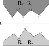
Figure 1.

We note that the arguments in the proof of Lemma 5.2 work for the arc in Proposition 5.4. Hence we have:

Lemma 5.5.

If $g$ strongly splits $f$, there exists $t$ such that $I\times\{t\}$ is disjoint from $(R_{X}\cup R_{x})\cup(R_{Y}\cup R_{y})$ and the restriction of $f$ to $Q_{t}$ is a Morse function such that for each regular value $s$, $P_{s}\cap Q_{t}$ contains a simple closed curve which is essential on $P_{s}$.

Corollary 5.6.

Let $t$ be as in Lemma 5.5. There is a subarc $[s_{0},s_{1}]\times\{t\}\subset I\times\{t\}$ such that:

• $(s_{0},t)\in$ {an edge of the graphic},

• $(s_{1},t)\in$ {an edge of the graphic}, and

• for any $s\in(s_{0},s_{1})$, $(s,t)\in R_{\phi}$, and for any small $\epsilon>0$, $((s_{0}-\epsilon),t)\in R_{A}$ and $((s_{1}+\epsilon),t)\in R_{B}$.

Proof.

By Lemma 5.5, $I\times\{t\}$ is disjoint from $(R_{X}\cup R_{x})\cup(R_{Y}\cup R_{y})$. By Lemma 4.5, a neighborhood of $(0,t)$ (resp. $(1,t)$) in $[0,1]\times\{t\}$ is contained in $R_{A}\cup R_{a}$ (resp. $R_{B}\cup R_{b}$). For an $s\in(0,1)$, if $(s,t)$ is contained in $R_{a}$ or $R_{b}$, then $(s,t)$ is contained in $R_{x}$ or $R_{y}$, a contradiction. Hence for a small $\epsilon>0$, $(\epsilon,t)$ (resp. $(1-\epsilon,t)$) is contained in $R_{A}$ (resp. $R_{B}$). Let $s_{1}=\sup\{s{\mid[0,s]\times\{t\}\in{R_{A}{\cup}R_{\phi}}}\}$ and $s_{0}=\sup\{s<s_{1}{\mid(s,t)\in{R_{A}}}\}$. Then by Lemma 4.4, $s_{0}{\neq}s_{1}$, and it is clear that the conclusion of Corollary 5.6 holds. ∎

6. The Reeb Graph

Given a compact, orientable surface $F$, let $\varphi$ : $F\rightarrow\mathbb{R}$ be a smooth function such that $\varphi\mid_{int(F)}$ is a Morse function and each component of $\partial F$ is level. Define the equivalence relation $\sim$ on points on $F$ by $x\sim y$ whenever $x,y$ are in the same component of a level set of $\varphi$. The Reeb graph corresponding to $\varphi$ is the quotient of $F$ by the relation $\sim$. As suggested by the name, the Reeb graph $F^{\prime}=F/\sim$ is a graph such that the edges of $F^{\prime}$ come from annuli in $F$ fibered by level loops, and that the valency one vertices correspond to center singularities, and the valency three vertices correspond to saddle singularities.

Let $f$ and $g$ be as in Section 5. Suppose that $Q$ is not isotopic to $P$, and we take $t$ as in Lemma 5.5. Let $G$ be the Reeb graph corresponding to $f\mid_{Q_{t}}$. There are two types of edges in $G$. If each point of an edge corresponds to an essential simple closed curve on $Q_{t}$, then the edge is called an essential edge. If each point of the edge corresponds to an inessential simple closed curve on $Q_{t}$, then the edge is called an inessential edge.

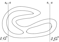
Figure 2.

Figure 3.

We continue with hypotheses of Section 5. Particularly, let $s_{0},s_{1},t$ be as in Corollary 5.6, hence, $[s_{0},s_{1}]\times\{t\}$ is an unlabelled interval in horizontal arc. For a small $\epsilon>0$, let $Q^{*}=f^{-1}(s_{0}+\epsilon,s_{1}-\epsilon)\cap Q_{t}$. Then $G^{*}$ denotes the Reeb graph corresponding to $f\mid_{Q^{*}}:Q^{*}\rightarrow I$. We say that a vertex of $G^{*}$ corresponding to a component of $\partial Q^{*}$ is a $\partial$-vertex. In particular, if a $\partial$-vertex corresponds to a component of $f^{-1}(s_{0}+\epsilon)\cap Q_{t}$ (resp. $f^{-1}(s_{1}-\epsilon)\cap Q_{t}$), then it is called a $\partial_{-}$-vertex (resp. $\partial_{+}$-vertex). The union of $\partial_{-}$-vertices (resp. $\partial_{+}$-vertices) is denoted by $\partial_{-}G^{*}$ (resp. $\partial_{+}G^{*}$). Let $f^{*}:G^{*}\rightarrow[s_{0}+\epsilon,s_{1}-\epsilon]$ be the function induced from $f\mid_{Q^{*}}:Q^{*}\rightarrow[s_{0}+\epsilon,s_{1}-\epsilon]$. Note that for each $s\in(s_{0}+\epsilon,s_{1}-\epsilon)$, $f^{*-1}(s)(\subset{G^{*}})$ consists of a finite number of points corresponding to the components of $P_{s}\cap{Q_{t}}$. Since $(s,t)$ is contained in an unlabelled region, there exists a component of $P_{s}{\cap}Q_{t}$ which is essential on both surfaces. This implies the next proposition.

Proposition 6.1.

Let $e$ be an inessential edge of $G^{*}$. For each $x\in e$, there exists an essential edge $e^{\prime}$ of $G^{*}$ such that $f^{*}(x)\in f^{*}(e^{\prime})$.

We consider local configurations of essential edges and inessential edges near a valency three vertex. At a valency three vertex, we may regard that an edge branches away two edges or that two edges are bound into one according to the parameter $s$ $(\in(s_{0}+\epsilon,s_{0}-\epsilon))$. We first consider the case of branching away (Figure 4). We take a point (e.g. $x_{1},x_{2}$ and $x_{3}$) in each edge adjacent to the vertex as in Figure 4. Then $c_{x_{i}}$ denotes the simple closed curve on $Q_{t}$ corresponding to $x_{i}$. Each $c_{x_{i}}$ is either essential or inessential on $Q_{t}$. We naively have six cases up to reflection in horizontal line. But the two cases in Figure 4 do not occur, because it is easy to see that if $c_{x_{1}}$ and $c_{x_{2}}$ (resp. $c_{y_{2}}$ and $c_{y_{3}}$) in Figure 4 are inessential simple closed curves on $Q_{t}$, then $c_{x_{3}}$ (resp. $c_{y_{1}}$) is also inessential.

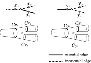
Figure 4.

Hence, the possible patterns of essential and inessential edges in neighborhoods of the vertices are shown in Figure 5 (1)–(4).

Type (1) shows that an essential edge branches away two essential edges and type (2) shows that an inessential edge branches away two essential edges. Type (3) shows that an essential edge branches away an essential edge and an inessential edge and type (4) shows that an inessential edge branches away two inessential edges.

Then we consider the case of binding into one edge. It is clear that possible cases are obtained from type (1)–(4) configurations by a horizontal reflection, which are shown in Figure 5 (5)–(8).

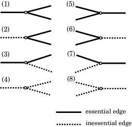
Figure 5.

7. An estimation of Hempel distance

Assigning positive integers to essential edges

Let $G^{*}$, $\partial_{\pm}G^{*}$, $f^{*}$ be as in Section 6. Let $G^{*}_{e}$ be the subgraph of $G^{*}$ consisting of the essential edges of $G^{*}$. Then $\partial_{\pm}G^{*}_{e}$ denotes the vertices of $G^{*}_{e}$ corresponding to $\partial_{\pm}G^{*}$. We assign a positive integer to each edge of $G^{*}_{e}$ according to the following steps. Let $v_{1},\dots,v_{k}$ be the vertices of $G^{*}_{e}$ which are not $\partial$-vertices. We suppose that $v_{1},\dots,v_{k}$ are positioned in this order from the left, i.e., $f^{*}(v_{1})<f^{*}(v_{2})<\dots<f^{*}(v_{k})$.

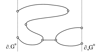
Figure 6.

Now we define Steps 0, 1 and 2 inductively for assigning positive integers to the edges of $G^{*}_{e}$.

Step 0. We assign $1$ to every edge adjacent to $\partial_{-}G^{*}_{e}$.

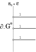
Figure 7.

Step 1. Suppose that there is a valency two vertex $v_{i}$ adjacent to edges $e_{l},e_{l^{\prime}}$ such that $e_{l}$ has already been assigned and $e_{l^{\prime}}$ has not been assigned yet. Then we assign the same integer as that of $e_{l}$ to $e_{l^{\prime}}$. We apply this assignment as much as possible.

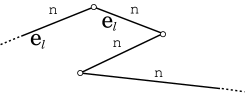
Figure 8.

In our assigning process, we will repeat applications of Steps 1 and 2. Before describing Step 2, we will give a general condition that the assignments have in the process. Suppose we finish Step 1 in repeated applications of Steps 1 and 2. At this stage, either every edge of $G^{*}_{e}$ is assigned exactly one integer, or there is a unique vertex $v_{i}$ such that there is an unassigned edge adjacent to $v_{i}$, and that each edge of $G_{e}^{*}$ containing a point $x$ with $f^{*}(x)<f^{*}(v_{i})$ has already been assigned exactly one integer. Then we suppose that the assigned integers satisfy the following conditions (*) and (**). (Note that the conditions are clearly satisfied after Steps 0 and 1.)

(*) For a small $\epsilon>0$, let $L_{i}$ be the set of the edges of $G^{*}_{e}$ each containing a point $x$ with $f^{*}(x)=f^{*}(v_{i})-\epsilon$. Then it satisfies one of the following conditions:

(1) All of the elements of $L_{i}$ are assigned with the same integer, say $n$.

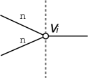
Figure 9.

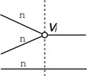
Figure 10.

(2) The set of the integers assigned to the elements of $L_{i}$ consists of consecutive two integers, say $n-1$ and $n$.

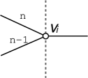
Figure 11.

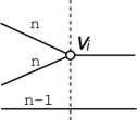
Figure 12.

(**) Moreover, if there exists an assigned edge of $G_{e}^{*}$ containing a point $p_{+}$ with $f^{*}(p_{+})>f^{*}(v_{i})$, then each such edge is assigned $n-1$ or $n$ as above. In particular, for a point $p_{-}$ with $f^{*}(p_{-})>f^{*}(v_{i})-\epsilon$, if all of the assigned edges each containing a point $x$ with $f^{*}(x)=f^{*}(p_{-})$ are assigned the same integer $n^{\prime}$ ($=n-1$ or $n$), then we have:

(i) all of the assigned edges containing a point $x_{+}$ with $f^{*}(x_{+})>f^{*}(p_{-})$ are assigned $n^{\prime}$, and

(ii) if a point $x^{*}$ with $f^{*}(x^{*})>f^{*}(p_{-})$ is contained in an assigned edge, then there is a point $x^{\prime}$ with $f^{*}(x^{\prime})=f^{*}(p_{-})$ and a path $\mathcal{P}$ in $G_{e}^{*}$ such that $\mathcal{P}$ is contained in a union of edges assigned $n^{\prime}$, and joins the points $x^{\prime}$ and $x^{*}$.

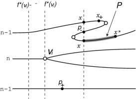
Figure 13.

Step 2.

1. Suppose that the vertex $v_{i}$ satisfies the condition (1). Then we assign $n+1$ to the unassigned edge(s) adjacent to $v_{i}$.

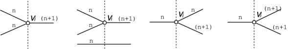
Figure 14.

2. Suppose that the vertex $v_{i}$ satisfies the condition (2). Then we assign $n$ to the unassigned edge(s) adjacent to $v_{i}$.

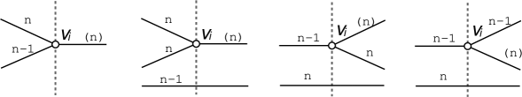
Figure 15.

After finishing Step 2, we apply Step 1. Then either all of the edges of $G^{*}_{e}$ are assigned integer(s), or there is a unique vertex $v_{j}$ such that there is an unassigned edge adjacent to $v_{j}$, and that each edge of $G^{*}_{e}$ that contains a point $y$ such that $f^{*}(y)<f^{*}(v_{j})$ has already been assigned. Here we note that there are no multiple assignments of integers for an edge and the above conditions (*) and (**) hold for the new assignment. That is:

Lemma 7.1.

At the stage, each edge of $G^{*}_{e}$ is assigned at most one integer, and we have the following.

(*)^′ For a small $\epsilon>0$, let $L_{j}$ be the set of the edges of $G^{*}_{e}$ each containing a point $y$ with $f^{*}(y)=f^{*}(v_{j})-\epsilon$. Then the assigned integers satisfy one of the following conditions:

(1)^′ All of the elements of $L_{j}$ are assigned with the same integer, say $m$.

(2)^′ The set of the integers assigned to the elements of $L_{j}$ consists of consecutive two integers, say $m-1,m$.

(**)^′ Moreover, if there exists an assigned edge of $G_{e}^{*}$ containing a point $q_{+}$ with $f^{*}(q_{+})>f^{*}(v_{j})$, then each such edge is assigned $m-1$ or $m$ as above. In particular, for a point $q_{-}$ with $f^{*}(q_{-})>f^{*}(v_{j})-\epsilon$, if all of the assigned edges each containing a point $y$ with $f^{*}(y)=f^{*}(q_{-})$ are assigned the same integer $m^{\prime}$ ($=m-1$ or $m$), then we have:

(i)^′ all of the assigned edges containing a point $y_{+}$ with $f^{*}(y_{+})>f^{*}(q_{-})$ are assigned $m^{\prime}$, and

(ii)^′ if a point $y^{*}$ with $f^{*}(y^{*})>f^{*}(q_{-})$ is contained in an assigned edge, then there is a point $y^{\prime}$ with $f^{*}(y^{\prime})=f^{*}(q_{-})$ and a path $\mathcal{Q}$ in $G_{e}^{*}$ such that $\mathcal{Q}$ is contained in a union of edges assigned $m^{\prime}$, and joins the points $y^{\prime}$ and $y^{*}$.

Proof.

Let $v_{i}$ be as above. We say that $v_{i}$ is of type (a) if at the stage just before applying the last Step 2, there does not exist an assigned edge of $G^{*}_{e}$ which contains a point $p$ such that $f^{*}(p)>f^{*}(v_{i})$. The vertex $v_{i}$ is said to be of type (b) if it is not of type (a). We say that $v_{j}$ is of type (a) if at the current stage, there does not exist an assigned edge of $G^{*}_{e}$ which contains a point $q$ such that $f^{*}(q)>f^{*}(v_{j})$. The vertex $v_{j}$ is said to be of type (b) if it is not of type (a).

We divide the proof into the following cases.

Case 1. The vertex $v_{i}$ is of type (a).

In this case, we note that $f^{*-1}(f^{*}(v_{i}))\cap$(the union of the assigned edges)$=v_{i}$, and that the valency of $v_{i}$ is three.

Case 1-1. The vertex $v_{i}$ satisfies the above condition (*)-(1).

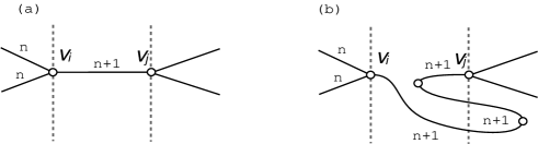
Figure 16.

In this case, it is clear that we have (*)^′-(1)^′ with $m=n+1$. Suppose $v_{j}$ is of type (a), then it is clear that (**)^′ holds. Suppose that $v_{j}$ is of type (b). Since the last assigning process is Step 1, all of the assigned edges containing a point $q$ with $f^{*}(q)>f^{*}(v_{i})$ are assigned $n+1$. This implies (**)^′ holds. We note that in this case, the all of the integers introduces in the process is $n+1$, and there is no possibility of multiple assignment.

Case 1-2. The vertex $v_{i}$ satisfies the above condition (*)-(2).

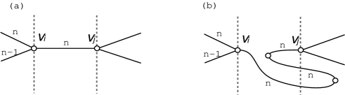
Figure 17.

In this case, we see that two edges bind into one edge at $v_{i}$, where an edge is assigned $n$ and the other is assigned $n-1$. We note that the same arguments as in Case 1-1 works, where the new integer is $n$.

Case 2. The vertex $v_{i}$ is of type (b).

Case 2-1. The vertex $v_{i}$ satisfies the above condition (*)-(1).

In this case, the set of the integers assigned to the edges of $G^{*}_{e}$ each of which contains a point $r$ with $f^{*}(r)=f^{*}(v_{i})+\epsilon$ consists of {$n$, $n+1$}. (Note that each edge is assigned at most one integer.) Since the assignment at the stage before applying the last Step 2 satisfies (**)-(i), the current assignment satisfies (*)^′-(1)^′ or (*)^′-(2)^′. Now we will see (**)^′ holds.

Case 2-1-1. The vertex $v_{j}$ satisfies (*)^′-(1)^′ with $m=n+1$.

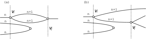
Figure 18.

In this case, we note that at the stage before applying the last Step 2, all of the assigned edges containing a point $r^{\prime}$ with $f^{*}(r^{\prime})>f^{*}(v_{i})$ are assigned $n$, and the integer introduced in the last Step 2 and Step 1 is $n+1$. Suppose $v_{j}$ is of type (a), then it is clear that (**)^′ holds (see Fig. 18(a)). Suppose that $v_{j}$ is of type (b) (see Fig. 18(b)). Since $v_{i}$ satisfies (**)-(ii), (**)^′-(i)^′ holds with $m^{\prime}=n+1$. Since the last assigning process is Step 1, we see that (**)^′-(ii)^′ holds.

Case 2-1-2. The vertex $v_{j}$ satisfies (*)^′-(1)^′ with $m=n$.

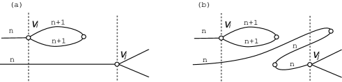
Figure 19.

In this case, we note that at the stage before applying the last Step 2, all of the assigned edges containing a point $r^{\prime}$ with $f^{*}(r^{\prime})>f^{*}(v_{i})$ are assigned $n$, and the integer introduced in the last Step 2 and Step 1 is $n+1$. Suppose $v_{j}$ is of type (a), then it is clear that (**)^′ holds (see Fig. 19(a)). Suppose that $v_{j}$ is of type (b). The condition of this case (Case 2-1-2) implies that the union of the edges assigned $n+1$ in these steps is a closed curve lying in the level less than $f^{*}(v_{j})$ (see Fig. 19(b)). Hence by (**)-(i), we see that $v_{j}$ satisfies (**)^′-(i)^′, and by (**)-(ii), we see that $v_{j}$ satisfies (**)^′-(ii)^′.

Case 2-1-3. The vertex $v_{j}$ satisfies (*)^′-(2)^′ with $m=n+1$.

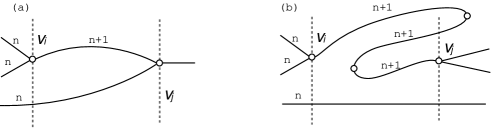
Figure 20.

In this case, we note that at the stage before applying the last Step 2, all of the assigned edges containing a point $r^{\prime}$ with $f^{*}(r^{\prime})>f^{*}(v_{i})$ are assigned $n$, and the integer introduced in the last Step 2 and Step 1 is $n+1$. Suppose $v_{j}$ is of type (a), then it is clear that (**)^′ holds. Suppose that $v_{j}$ is of type (b). By (**) and the fact that the integer introduced in the last Step 2 and Step 1 is $n+1$, we see that $v_{j}$ satisfies (**)^′.

Case 2-2. The vertex $v_{i}$ satisfies the above condition (*)-(2).

In this case, the set of the integers assigned to each edge of $G^{*}_{e}$ containing a point $r$ with $f^{*}(r)=f^{*}(v_{i})+\epsilon$ is either {$n$} or {$n-1$, $n$}. (Note that each edge is assigned at most one integer.)

Case 2-2-1. The set of the integers assigned to each edge of $G^{*}_{e}$ containing a point $r$ with $f^{*}(r)=f^{*}(v_{i})+\epsilon$ is {$n$}.

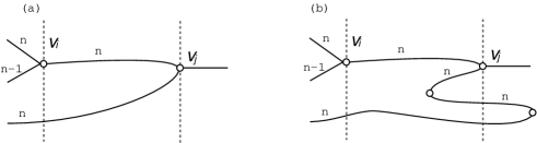
Figure 21.

In this case, by (**), we see that in the current assignment, each edge of $G^{*}_{e}$ containing a point $r^{\prime}$ with $f^{*}(r^{\prime})>f^{*}(v_{i})$ is assigned $n$. Suppose $v_{j}$ is of type (a), then it is clear that (**)^′ holds (see Fig. 21(a)). Suppose that $v_{j}$ is of type (b) (see Fig. 21(b)). By (**) and the fact that the integer introduced in the last Step 2, and Step 1 is $n$, we see that $v_{j}$ satisfies (**)^′.

Case 2-2-2. The set of the integers assigned to each edge of $G^{*}_{e}$ containing a point $r$ with $f^{*}(r)=f^{*}(v_{i})+\epsilon$ is {$n-1,n$}.

In this case, by using the argument as in Case 2-1, we see that $v_{j}$ satisfies (*)^′-(1)^′ or (*)^′-(2)^′, and (**)^′. This completes the proof of the lemma. ∎

By Lemma 7.1, we can apply Step 2 and Step 1 again and repeat the procedure until all the edges of $G^{*}_{e}$ assigned.

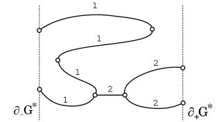
Figure 22.

Recall that $v_{1},\dots,v_{k}$ are the vertices of $G^{*}_{e}$ which are not $\partial$-vertices such that $f^{*}(v_{1})<f^{*}(v_{2})<\dots<f^{*}(v_{k})$. Let $r_{0}=s_{0}-\epsilon$ and $r_{k+2}=s_{1}+\epsilon$. Then we fix levels $r_{1},\dots,r_{k+1}$ such that $s_{0}<r_{1}<f^{*}(v_{1})$, $f^{*}(v_{i})<r_{i+1}<f^{*}(v_{i+1})$ $(i=1,\dots,k-1)$, and $f^{*}(v_{k})<r_{k+1}<s_{1}$. We consider the system of simple closed curves in $P_{r_{i}}\cap Q_{t}$ on $P_{r_{i}}$. Since there is a continuous deformation from $P_{r_{i}}$ to $P_{r_{i+1}}$, that is the sweep-out, we may regard $P_{r_{1}}\cap Q_{t}$,…, $P_{r_{k+1}}\cap Q_{t}$ are systems of simple closed curves on $P$. Recall that $(r_{0},t)$ is contained in a region labelled $A$. Let $c_{0}$ be the simple closed curve in $P_{r_{0}}\cap Q_{t}$ which bounds a meridian disk in $A$, and let $c_{*}$ be an essential simple closed curve in $P$ corresponding to an edge $e_{*}$ of $G^{*}_{e}$ (that is, $c_{*}$ is a component of $P_{r_{i}}\cap{Q_{t}}$ for some $i$).

Lemma 7.2.

$d_{P}(c_{0},c_{*})$ is at most the integer assigned to $e_{*}$.

Proof.

We prove the lemma by following the assigning process for the edges of $G^{*}_{e}$ in this section.

We consider the intersection $P_{r_{i}}\cap Q_{t}$. Let $C_{i}$ be the union of the components of $P_{r_{i}}\cap Q_{t}$ which are essential on $P_{r_{i}}$. Since $(s_{0},s_{1})\times\{t\}$ is an unlabelled interval, each component of $C_{i}$ is essential on $Q_{t}$. The isotopy class of $C_{i+1}$ in $P_{r_{i+1}}$ is obtained from the isotopy class of $C_{i}$ in $P_{r_{i}}$ by a band move, or addition or deletion of a pair of simple closed curves which are parallel on $Q_{t}$. Hence we see that the distance between $c_{0}$ and each element of $C_{1}$ is at most 1. This observation represents the assignment of integer 1 in Step 0.

Then we consider about Step 1. Suppose that there is a valency two vertex $v_{i}$ adjacent to edges $e_{l},e_{l^{\prime}}$ such that $e_{l}$ has already been assigned and $e_{l^{\prime}}$ has not been assigned yet. Let $c_{l}$ (resp. $c_{l^{\prime}}$) be the simple closed curve corresponding to $e_{l}$ (resp. $e_{l^{\prime}}$). Note that $c_{l},c_{l^{\prime}}$ are pairwise parallel essential simple closed curves on $Q_{t}$. Hence $c_{l}\cup c_{l^{\prime}}$ bounds an annulus, say $\mathcal{A}$ in $Q_{t}$.

Claim. The simple closed curves $c_{l},c_{l^{\prime}}$ are isotopic on $P$.

Proof. Since $[s_{0}+\epsilon,s_{1}-\epsilon]\times\{t\}$ goes though unlabelled regions, each component of int$\mathcal{A}\cap{P_{s_{0}+\epsilon}}$ (resp. int$\mathcal{A}\cap{P_{s_{1}-\epsilon}}$) is a simple closed curve that is inessential in both $\mathcal{A}$ and $P_{s_{0}+\epsilon}$ (resp. $\mathcal{A}$ and $P_{s_{1}-\epsilon}$). By using innermost disk arguments if necessary, we may suppose $\mathcal{A}$ is completely contained in $P\times[s_{0}+\epsilon,s_{1}-\epsilon]$. This annulus gives a free homotopy from $c_{l}$ to $c_{l^{\prime}}$ on $P$. This show that $c_{l}$ and $c_{l^{\prime}}$ are isotopic on $P$.

The above claim shows that the assigning rule in Step 1 is natural.

Now we consider about Step 2. Let $c_{r}$ be the simple closed curve corresponding to the point $r$ with $f^{*}(r)=f^{*}(v_{i})-\epsilon$ and $c_{l}$ be the simple closed curve corresponding to the point $l$ with $f^{*}(l)=f^{*}(v_{i})+\epsilon$. Recall that the isotopy class of $C_{i+1}$ is obtained from the isotopy class of $C_{i}$ by a band move, or addition or deletion of a pair of simple closed curves which are parallel on $Q_{t}$. Hence $c_{l}$ is ambient isotopic to simple closed curves disjoint from $c_{r}$.

Suppose that $v_{i}$ satisfies the condition (*)-(1) in this section. Since an edge containing the point $x$ is assigned $n$, $d_{P}(c_{0},c_{x})\leq{n}$. Note that $c_{l}$ is disjoint from $c_{r}$. Hence $d_{P}(c_{0},c_{l})\leq{n+1}$. Recall that $n+1$ is the number assigned to $e_{l}$.

Suppose that $v_{i}$ satisfies the condition (*)-(2) in this section. We may suppose that the edge containing $r$ is assigned $n-1$, hence $d_{P}(c_{0},c_{r})\leq{n-1}$. Note that $c_{l}$ is disjoint from $c_{r}$. Hence $d_{P}(c_{0},c_{l})\leq{n}$. Recall that $n$ is the number assigned to $e_{l}$. This completes the proof of the lemma. ∎

Now, we give the proof of the next theorem.

Theorem 7.3.

Let $P,Q$ and $G^{*}_{e}$ be as above. Let $n$ be the minimum of the integers assigned to the edges adjacent to $\partial_{+}G^{*}_{e}$. Then the distance $d(P)$ is at most $n+1$.

Proof.

Let $r_{0},\dots,r_{k+2}$ be as above. Recall that $P_{r_{0}}\cap Q_{t}$ contains a simple closed curve, say $c_{0}$ which bounds a meridian disk of $A$. On the other hand, $P_{r_{k+2}}\cap Q_{t}$ contains a simple closed curve, say $c_{k+2}$ which bounds a meridian disk of $B$. By Lemma 7.2, we see that $d(c_{0},c^{\prime})\leq n$, for a component $c^{\prime}$ of $P_{r_{k+1}}\cap{Q_{t}}$. Note that $c^{\prime}$ is disjoint from $c_{k+2}$. Hence $d_{P}(c_{0},c_{k+2})\leq n+1$. This implies that $d(P)\leq n+1$.
∎

References

- [1] M. Golubitsky and V. Guillemin, Stable mappings and their singularities, Graduate Texts in Math., 14 (1973), Springer-Verlag, New York, Heidelberg, Berlin.
- [2] W. J. Harvey, Boundary structure of the modular group. In Riemann surfaces and related topics, Proceedings of the 1978 Stony Brook Conference (State Univ. New York, Stony Brook, N.Y., 1978), pages 245-251, Princeton, N.J., 1981. Princeton Univ. Press.
- [3] J. Hempel, 3-manifolds as viewed from the curve complex, Topology 40 (2001), no. 3, 631-657.
- [4] M.W. Hirsch, Differential topology, Graduate Texts in Math., 33 (1976), Springer- Verlag, New York, Heidelberg, Berlin.
- [5] J. Hass, A. Thompson, W. Thurston, Stabilization of Heegaard splittings, preprint (2008), ArXiv:math.GT/0802.2145v2
- [6] J. Johnson, Stable functions and common stabilizations of Heegaard splittings, Trans. Amer. Math. Soc. 361 (2009), no. 7, 3747–3765.
- [7] J. Johnson, Flipping and stabilizing Heegaard splittings, preprint (2008), ArXiv: math.GT/08054422.
- [8] J.N. Mather, Stability of mappings, V: Transversality, Adv. Math., 4 (1970), 301-336.
- [9] T. Kobayashi and O. Saeki, The Rubinstein-Scharlemann graphic of a 3-manifold as the discriminant set of a stable map, Pacific J. Math. 195 (2000), no. 1, 101-156.
- [10] H. Rubinstein and M. Scharlemann, Comparing Heegaard splittings of non-Haken 3-manifolds, Topology 35 (1996), no. 4, 1005-1026.
- [11] M. Scharlemann and M. Tomova, Alternate Heegaard genus bounds distance, Geom. Topol. 10 (2006) 593–617.
- [12] T. Li, Saddle tangencies and the distance of Heegaard splittings, Algebr. Geom. Topol. 7 (2007), 1119–1134.
- [13] F. Waldhausen, On irreducible 3-manifolds which are sufficiently large, Ann. of Math. 87 (1968), 56-88.