Quantum electrodynamics of one-photon wave packets

I Introduction

Excited bound states of atoms are one of the simplest examples of unstable quantum states which decay radiatively into the continuum of possible one-photon states of the electromagnetic field in free space. The search for a satisfactory theoretical explanation of the line frequencies and intensities of photon emission spectra at the beginning of the last century eventually culminated in Heisenberg’s ’magical paper’ from July 1925 Heisenberg ; Aitchison and in the development of modern quantum mechanics Born ; Schroedinger1 ; Schroedinger2 ; Dirac . Although basic aspects of this spontaneous decay process have already been described theoretically in an adequate way in the early days of modern quantum mechanics WignerWeisskopf1 ; WignerWeisskopf2 , interestingly, some of its time-dependent dynamical aspects are still of topical current interest.

To a large part the current interest in this elementary photon emission process is due to recent advances in quantum technology. They have enabled one to prepare quantum states of matter and of the electromagnetic field to such a high level of precision that not only subtle quantum electrodynamical phenomena can be tested experimentally but that these phenomena can also be exploited practically for purposes of quantum information processing quantuminfoproc . On the one hand it is possible to engineer quantum states of individual atoms or even of multi-particle systems with the help of sophisticated particle traps. In this context electromagnetic fields play a predominant role for achieving the required trapping and they also allow to control the material quantum states involved with an unprecedented level of accuracy trappedatoms1 ; trappedatoms2 . On the other hand it is also possible to engineer quantum states of the electromagnetic field. Not only classical electromagnetic fields with large photon numbers can be generated by sophisticated pulse shaping techniques pulseshape but also particular few-photon quantum states of the electromagnetic field can be prepared in a controlled way. In the context of cavity quantum electrodynamics CQED , for example, extreme selection of electromagnetic field modes by cavities in combination with trapping of single atoms even enables one to control the interaction between single atoms and the electromagnetic field. Thus, it is possible to prepare single-photon single-mode quantum states of the electromagnetic field onephoton , for example, or to excite a single atom by a single-photon quantum state perfectly with the help of vacuum Rabi oscillations Schleich . Despite these significant advances of quantum electrodynamics similarly efficient techniques for preparing many-mode few-photon quantum states of the electromagnetic field or for controlling the resulting atom-field dynamics are significantly less well developed. Advances in this direction would be particularly interesting for purposes of quantum information processing. They would significantly enhance the flexibility of exchanging quantum information between the electromagnetic field, which is particularly useful for the transport of quantum information, and matter, which is well suited for the storage of quantum information.

In this contribution we investigate quantum electrodynamical many-mode aspects by exploring the simplest possible situation in this context, namely the interaction of a single atom, modeled by a simple two-level system, with many-mode one-photon quantum states of the electromagnetic field Quabis . In particular, we concentrate on the question how the engineering of electromagnetic field modes influences the atom-field interaction. An interesting problem in this context is the engineering of ideal one-photon multi-mode quantum states which may excite a single atom perfectly StobAlLeu . For purposes of quantum information processing such one-photon multi-mode states are particularly well suited for transmitting quantum information and for storing it in a material memory again.

This article is organized as follows: In Sec. II characteristic aspects of two extreme cases of the interaction of a simple two-state quantum system with the radiation field are discussed, namely the single-mode Jaynes-Cummings-Paul model JCP1 ; JCP2 and spontaneous photon emission in free space WignerWeisskopf1 ; WignerWeisskopf2 . In Sec. III we explore dynamical modifications originating from modifications of the electromagnetic field modes involved. For this purpose the interaction of a single photon with a two-level system in a closed spherical cavity of arbitrary size Alber1992 and in a half-open parabolic cavity Sondermann2007 ; Maiwald are explored.

II Quantum electrodynamics of a material two-level system - basic aspects

In this section basic results concerning the interaction of matter with the quantized radiation field are discussed. For this purpose an elementary two-level model of matter is considered with involves two non-degenerate relevant energy eigenstates which are coupled almost resonantly to the electromagnetic field. Characteristic quantum electrodynamical properties of this model system are particularly apparent in cases in which the quantum states of the electromagnetic field contain only a small number of photons. The resulting dynamics depends significantly on whether only one mode of the radiation field or an infinite number of them participate in the interaction.

II.1 The Jaynes-Cummings-Paul model

One of the simplest models which describes characteristic quantum features of the almost resonant interaction of matter with the radiation field is the Jaynes-Cummings-Paul model JCP1 ; JCP2 . In this model a material two-level system interacts with a single mode of the radiation field. In the Schrödinger picture its dynamics is described by the Hamiltonian

$$\hat{H} = E_{g}|g\rangle\langle g|+E_{e}|e\rangle\langle e|+\hbar\omega\hat{a}^{\dagger}\hat{a}+\hbar g\hat{a}|e\rangle\langle g|+\hbar g^{*}\hat{a}^{\dagger}|g\rangle\langle e|.$$ (1)

The energies of the material two-level system are denoted by $E_{g}$ and $E_{e}>E_{g}$ and $\hat{a}$ ($\hat{a}^{\dagger}$) is the destruction (creation) operator of the almost resonantly coupled electromagnetic field mode of frequency $\omega$, i.e. $E_{e}-E_{g}\approx\hbar\omega$. The coupling constant $g$ characterizes the strength of the interaction of the material two-level system with the single mode of the radiation field. In the dipole approximation, for example, which applies in typical quantum optical situations and in which it is assumed that the wavelength of the almost resonantly coupled electromagnetic field mode is significantly larger than the extension of the material charge distribution of the two-level system, this coupling constant is given by

$$\hbar g\hat{a} = -\langle e|\hat{{\bf d}}|g\rangle\cdot\hat{{\bf E}}_{+}({\bf x}_{0}).$$ (2)

Thereby, $\hat{{\bf d}}$ is the material dipole operator. The positive frequency component of the electric field operator is denoted by

$$\hat{{\bf E}}_{+}({\bf x}) = i\sqrt{\frac{\hbar\omega}{2\epsilon_{0}}}{\bf u}({\bf x})\hat{a},$$ (3)

and it has to fulfill the transversality condition $\nabla\cdot\hat{{\bf E}}_{+}({\bf x})=0$. ( $\epsilon_{0}$ is the permittivity of the vacuum.) The normalized mode function ${\bf u}({\bf x})$ is a solution of the Helmholtz equation

$$\left(\nabla^{2}+\omega/c^{2}\right){\bf u}({\bf x}) = 0$$ (4)

and fulfills the boundary conditions of the mode selecting cavity involved. It is normalized according to the relation $\int_{\mathbb{R}^{3}}d^{3}x~{}|{\bf u}({\bf x})|^{2}=1$. The position of the center-of-mass of the material charge distribution is denoted by ${\bf x}_{0}$.

Within this model the dynamics of the almost resonantly coupled matter-field system can be described in a straight forward way by expanding the quantum state $|\psi\rangle_{t}$ at time $t$ in the basis of energy eigenstates of the uncoupled quantum system, i.e.

$$|\psi\rangle_{t} = \sum_{n=0}^{\infty}\{a_{e,n}(t)e^{-i(E_{e}+n\hbar\omega)t/\hbar}|e\rangle\otimes|n\rangle+a_{g,n}(t)e^{-i(E_{g}+n\hbar\omega)t/\hbar}|g\rangle\otimes|n\rangle\}.$$ (5)

The time-dependent Schrödinger equation $i\hbar d|\psi\rangle_{t}/dt=\hat{H}|\psi\rangle_{t}$ yields the system of pairs of coupled equations

$$\dot{a}_{e,n}(t) = -ig\sqrt{n+1}e^{i\Delta t}a_{g,n+1}(t),$$

$$\dot{a}_{g,n+1}(t) = -ig^{*}\sqrt{n+1}e^{-i\Delta t}a_{e,n}(t)~{}~{}({\rm for}~{}~{}n\geq-1)$$ (6)

with $\Delta=(E_{e}-\hbar\omega-E_{g})/\hbar$ denoting the detuning from resonance.

If initially, at $t=0$, the two-level system is prepared in its excited state $|e\rangle$, i.e. $a_{g,n}(0)=0$ for $n\geq 0$, Eqs.(6) yield the solution

$$a_{e,n}(t) = a_{e,n}(0)\left(\cos\left(\frac{\Omega_{n}t}{2}\right)-\frac{i\Delta}{\Omega_{n}}\sin\left(\frac{\Omega_{n}t}{2}\right)\right)e^{i\Delta t/2},$$

$$a_{g,n+1}(t) =- a_{e,n}(0)\frac{2ig^{*}\sqrt{n+1}}{\Omega_{n}}\sin\left(\frac{\Omega_{n}t}{2}\right)e^{-i\Delta t/2}.$$ (7)

The time evolution of the probability amplitudes $a_{e,n}(t)$ and $a_{g,n}(t)$ exhibits a characteristic periodic energy transfer between the two-level system and the electromagnetic field mode which is characterized by the $n$-photon Rabi frequency $\Omega_{n}=\sqrt{\Delta^{2}+4|g|^{2}(n+1)}$. As the period of this energy exchange depends on the photon number the resulting time evolution exhibits interesting collapse and revival phenomena.

Let us consider a special case in more detail in which initially the two-level system is excited and the single-mode radiation field is in a coherent state $|\alpha\rangle$ with $\hat{a}|\alpha\rangle=\alpha|\alpha\rangle$ and $\alpha\in{\mathbb{C}}$ Schleich . The resulting time evolution of the inversion of the two-level system is given by

$$w(t) := \sum_{n=0}^{\infty}\{|a_{e,n}(t)|^{2}-|a_{g,n}(t)|^{2}\}=\sum_{n=0}^{\infty}|a_{e,n}(0)|^{2}\left(\frac{\Delta^{2}}{\Omega_{n}^{2}}+\frac{4|g|^{2}(n+1)}{\Omega_{n}^{2}}\cos\left(\Omega_{n}t\right)\right)$$

with $a_{e,n}(0)={\rm exp}(-|\alpha|^{2}/2)\alpha^{n}/\sqrt{n!}$. In Fig.(1) the time evolution of this inversion is depicted for resonant coupling, i.e. $\Delta=0$, and various values of the mean photon number $<n>=\langle\alpha|\hat{a}^{\dagger}\hat{a}|\alpha\rangle=|\alpha|^{2}$ of a coherent state $|\alpha\rangle$. It is apparent that the initially prepared inversion collapses after a characteristic collapse time of the order of $T_{c}=2\pi/|g|$. Furthermore, at multiples of times of the order of $T_{r}=2\pi\sqrt{<n>+1}/|g|$ the probability amplitudes interfere constructively again thus causing revivals of the initial excitation revivals1 ; revivals2 . Finally, it should also be mentioned that according to Eq.(LABEL:inversion) the appearance of collapse and revival phenomena do not necessarily require an initially prepared pure quantum state of the electromagnetic field.

Figure 1: Time dependence of the inversion $w(t)$ of Eq.(LABEL:inversion) of the two-level system describing its excitation by a coherent single-mode state $|\alpha\rangle$: $<n>=0.5$ (left curve), $<n>=25$ (right curve).

If one considers the extreme case that the two-level system is excited initially but the electromagnetic field is in its ground (vacuum) state one obtains the result

$$w(t) = \frac{\Delta^{2}}{\Omega_{0}^{2}}+\frac{4|g|^{2}}{\Omega_{0}^{2}}\cos(\Omega_{0}t)$$ (9)

for the inversion of the two-level system. In this case the inversion oscillates periodically between its extreme values and these oscillations are governed by the vacuum Rabi frequency $\Omega_{0}=2|g|$. In particular, this result demonstrates that in the case of the coupling of a two-level system to a single mode of the radiation field the decay of the excited state of the two-level system is not described by an exponential decay law but exhibits a periodic energy exchange which reflects the periodic exchange of a photon between the two-level system and the radiation field.

II.2 Spontaneous emission of a photon in free space

If a material two-level system interacts with the quantized radiation field in free space its dynamics differs significantly from the single-mode case described previously. In order to exemplify these significant differences let us assume that initially the two-level system is prepared in its excited state $|e\rangle$ and that the electromagnetic field is in its ground (vacuum) state $|0\rangle$. In the absence of any mode-selecting cavity all modes of the electromagnetic radiation field couple to this initially excited two-level system. In the Schrödinger picture the field operators of the electric and magnetic field strengths are given by QED

$$\hat{{\bf E}}({\bf x}) = \sum_{{\bf k},i}\sqrt{\frac{\hbar\omega_{{\bf k}}}{2\epsilon_{0}}}\{i{\bf u}_{{\bf k},i}({\bf x})\hat{a}_{{\bf k},i}-i{\bf u}^{*}_{{\bf k},i}({\bf x})\hat{a}^{\dagger}_{{\bf k},i}\}=\hat{{\bf E}}_{+}({\bf x})+\hat{{\bf E}}_{-}({\bf x}),$$ (10)

$$\hat{{\bf B}}({\bf x}) = \sum_{{\bf k},i}\sqrt{\frac{\hbar}{2\epsilon_{0}\omega_{{\bf k}}}}\{(\nabla\wedge{\bf u}_{{\bf k},i})({\bf x})\hat{a}_{{\bf k},i}+(\nabla\wedge{\bf u}^{*}_{{\bf k},i})({\bf x})\hat{a}^{\dagger}_{{\bf k},i}\}=\hat{{\bf B}}_{+}({\bf x})+\hat{{\bf B}}_{-}({\bf x})$$

with their corresponding ’positive-’ and ’negative-frequency’ parts $\hat{{\bf E}}_{+}({\bf x})$ and $\hat{{\bf E}}_{-}({\bf x})$ ( $\hat{{\bf B}}_{+}({\bf x})$ and $\hat{{\bf B}}_{-}({\bf x})$). If we consider an electromagnetic field in a cubic quantization volume of length $L$ and volume $V=L^{3}$ and impose periodic boundary conditions a complete set of orthonormal mode functions can be chosen in the form

$${\bf u}_{{\bf k},i}({\bf x}) = {\bf e}_{i}({\bf k})\frac{e^{i{\bf k}\cdot{\bf x}}}{\sqrt{V}},~{}i=1,2$$ (11)

with the wave vectors ${\bf k}=2\pi{\bf n}/L$ (${\bf n}\in{\mathbb{Z}}^{3})$ and with the corresponding real-valued unit-polarization vectors ${\bf e}_{i}({\bf k})$ (${\bf e}_{1}({\bf k})\cdot{\bf e}_{2}({\bf k})=0$, ${\bf e}_{1}({\bf k})\wedge{\bf e}_{2}({\bf k})={\bf k}/|{\bf k}|$) fulfilling the transversality condition ${\bf e}_{i}({\bf k})\cdot{\bf k}=0$ for $i=1,2$. Within a perturbative treatment of the spontaneous photon emission process according to Fermi’s Golden rule the resulting decay of the two-level system is governed by the rate QED

$$\Gamma = \sum_{{\bf k},i}\frac{2\pi}{\hbar}\mid\langle e|\hat{{\bf d}}|g\rangle\cdot\hat{{\bf E}}_{+}({\bf x}_{0})\mid^{2}\delta(E_{g}+\hbar\omega_{{\bf k}}-E_{e})=\frac{\omega_{eg}^{3}|\langle e|\hat{{\bf d}}|g\rangle|^{2}}{3\pi\epsilon_{0}\hbar c^{3}}$$

with the transition frequency $\omega_{eg}=\omega_{eg}$. Within the framework of the dipole approximation ${\bf x}_{0}$ denotes the position of the center-of-mass of the two-level system. It is apparent from Eq.(LABEL:spontdec) that the spontaneous decay rate depends on the number of field modes per unit energy which couple resonantly, i.e. with $\omega_{{\bf k}}=(E_{e}-E_{g})/\hbar$, to the spontaneously decaying two-level system. Thus, altering the mode structure of these relevant field modes by a cavity, for example, modifies the spontaneous decay rate. This effects was confirmed in experiments with Rydberg atoms of sodium Haroche83 excited in a niobium superconducting cavity. Rydberg atoms are especially suitable for the experimental verification of modifications of spontaneous decay rates since they posses large dipole matrix element on micro-wave transitions. Therefore, the spontaneous emission rate for the atomic transition 23S$\to$22P was investigated which was in resonance with the niobium superconducting cavity at $340$GHz. Thus, the free-space value of $\Gamma=150\mathrm{s}^{-1}$ could be increased to a value of $\Gamma_{cavity}=8\cdot 10^{4}\mathrm{s}^{-1}$.

A non-perturbative treatment of the exponential decay of an excited two-level system has already been given by Weisskopf and Wigner WignerWeisskopf1 ; WignerWeisskopf2 in their seminal work. If the initially prepared quantum state of the matter-field system is of the form $|e\rangle\otimes|0\rangle$ the time evolution of the resulting quantum state can be decomposed according to

$$|\psi\rangle_{t} = \sum_{{\bf k},i}a_{g{\bf k}i}(t)e^{-i(E_{g}+\hbar\omega_{{\bf k}})t/\hbar}|g\rangle\otimes\hat{a}^{\dagger}_{{\bf k},i}|0\rangle+a_{e}(t)e^{-iE_{e}t/\hbar}|e\rangle\otimes|0\rangle.$$ (13)

The resulting dynamics is described by the time dependent Schrödinger equation with Hamiltonian

$$\hat{H} = E_{g}|g\rangle\langle g|+E_{e}|e\rangle\langle e|+\sum_{{\bf k}\in I,i}\hbar\omega_{{\bf k}}\hat{a}^{\dagger}_{{\bf k},i}\hat{a}_{{\bf k},i}-$$ (14)

$$|e\rangle\langle g|~{}\langle e|\hat{{\bf d}}|g\rangle\cdot\hat{{\bf E}}_{+}({\bf x}_{0})-|g\rangle\langle e|~{}\langle e|\hat{{\bf d}}|g\rangle^{*}\cdot\hat{{\bf E}}_{-}({\bf x}_{0})$$

in the dipole- and rotating-wave approximation QED . The rotating wave approximation takes into account the interaction of the two-level system with the almost resonant field modes (${\bf k}\in I$) within a frequency interval of width $\Delta\omega\gg\Gamma$ centered around the transition frequency $\omega_{eg}$ in a non-perturbative way. The influence of all other (non-resonant) field modes can be taken into account perturbatively. In particular, in second order perturbation theory these non-resonant modes give rise to a Lamb shift Lambshift1 ; Lambshift2 . It should be mentioned that, contrary to the almost resonant modes, for a consistent treatment of this energy shift the coupling of the non-resonant modes of the radiation field to the two-level atom cannot be treated in the dipole approximation because also high-frequency field modes have to be taken into account. Furthermore, mass renormalization has to be included. This way a well-defined and finite expression for the Lamb shift can even be obtained within a non-relativistic quantum electrodynamical description Lambshift2 .

The time dependent Schrödinger equation is equivalent to the differential equations

$$\dot{a}_{e}(t) = -\frac{\langle e|\hat{{\bf d}}|g\rangle}{\hbar}\sum_{{\bf k}\in I,i}\sqrt{\frac{\hbar\omega_{{\bf k}}}{2\epsilon_{0}}}{\bf u}_{{\bf k},i}({\bf x}_{0})a_{g{\bf k}i}(t)e^{i(E_{e}-E_{g}-\hbar\omega_{{\bf k}})t/\hbar},$$

$$\dot{a}_{g{\bf k}i}(t) = \frac{\langle e|\hat{{\bf d}}|g\rangle^{*}}{\hbar}\sqrt{\frac{\hbar\omega_{{\bf k}}}{2\epsilon_{0}}}{\bf u}_{{\bf k},i}^{*}({\bf x}_{0})a_{e}(t)e^{-i(E_{e}-E_{g}-\hbar\omega_{{\bf k}})t/\hbar}$$ (15)

for the probability amplitudes which yield the integro-differential equation

$$a_{e}(t) = -\sum_{{\bf k}\in I,i}{\frac{\hbar\omega_{{\bf k}}|\langle e|\hat{{\bf d}}|g\rangle\cdot{\bf u}_{{\bf k},i}({\bf x}_{0})|^{2}}{2\hbar^{2}\epsilon_{0}}}\int_{0}^{t}dt^{\prime}~{}a_{e}(t^{\prime})e^{i(E_{e}-E_{g}-\hbar\omega_{{\bf k}})(t-t^{\prime})/\hbar}$$ (16)

for the probability amplitude $a_{e}(t)$ of observing the two-level system in its excited state $|e\rangle$ at time $t>0$. In the continuum limit of a large quantization volume $V$ the summation over the modes of the electromagnetic field can be approximated by

$$\sum_{{\bf k}\in I,i} \longrightarrow \sum_{i}\frac{V}{(2\pi)^{3}}\int_{{\bf k}\in I}d^{3}{\bf k}=\sum_{i}\int_{\omega\in I}d\omega\rho(\omega)$$ (17)

with $\rho(\omega)=4\pi V\omega^{2}/(8\pi^{3}c^{3})$ enumerating the number of field modes per frequency and per polarization. As long as the spontaneous decay rate $\Gamma$ of Eq.(LABEL:spontdec) is much smaller than the resonance frequency $\omega_{eg}$ and the frequency range over which the integrand of Eq.(16) varies significantly, the ’pole approximation’ WignerWeisskopf1 ; WignerWeisskopf2 ; pole may by applied so that Eq.(16) reduces to

$$a_{e}(t) = -\int_{0}^{t}dt^{\prime}~{}\Gamma a_{e}(t^{\prime})\delta(t-t^{\prime})=-\frac{\Gamma}{2}a_{e}(t).$$ (18)

Within this approximation the initially excited two-level atom decays exponentially with rate (LABEL:spontdec) so that for $t>0$ the quantum state is given by

$$|\psi\rangle_{t} = \sum_{{\bf k}\in I,i}(-i)\langle e|\hat{{\bf d}}|g\rangle^{*}\cdot{\bf u}^{*}_{{\bf k},i}({\bf x}_{0})\sqrt{\frac{\hbar\omega_{{\bf k}}}{2\epsilon_{0}}}\frac{e^{-i(E_{g}+\hbar\omega_{{\bf k}})t/\hbar}-e^{-i(E_{e}-i\hbar\Gamma/2)t/\hbar}}{E_{e}-E_{g}-\hbar\omega_{{\bf k}}-i\hbar\Gamma/2}\hat{a}^{\dagger}_{{\bf k},i}|0\rangle\otimes|g\rangle+$$ (19)

$$e^{-i(E_{e}-i\hbar\Gamma/2)t/\hbar}|e\rangle\otimes|0\rangle.$$

Thus, at the end of the spontaneous decay process the two-level system approaches a separable pure quantum state with the two-level system in its lower energy eigenstate $|g\rangle$. In this quantum state the mean electric and magnetic field strengths vanish so that the (normally ordered) energy density of the electromagnetic field provides a local measure for the statistical uncertainty of these electromagnetic field strengths.

According to Eq.(19) after the completion of the photon emission process both the two-level system and the electromagnetic field are in pure states. In view of this asymptotic separation it is of interest to ask whether a one-photon state of the electromagnetic field exists which is capable of exciting a material system, such as an atom, perfectly in free space from an initially prepared ground state $|g\rangle$ to an excited state $|e\rangle$ by photon absorption. Within our quantum electrodynamical model this question can be answered in the affirmative in a straight forward way . For this purpose one has to solve Eqs.(15) subject to the final-state condition that at a particular time, say $t=0$, the two-level system is in its excited state and the radiation field in its vacuum state. It is straight forward to show that for $t\leq 0$ this advanced solution of Eqs.(15) is given by the quantum state

$$|\psi\rangle_{t} = \sum_{{\bf k}\in I,i}(-i)\langle e|\hat{{\bf d}}|g\rangle^{*}\cdot{\bf u}^{*}_{{\bf k},i}({\bf x}_{0})\sqrt{\frac{\hbar\omega_{{\bf k}}}{2\epsilon_{0}}}\frac{e^{-i(E_{g}+\hbar\omega_{{\bf k}})t/\hbar}-e^{-i(E_{e}+i\hbar\Gamma/2)t/\hbar}}{E_{e}-E_{g}-\hbar\omega_{{\bf k}}+i\hbar\Gamma/2}\hat{a}^{\dagger}_{{\bf k},i}|0\rangle\otimes|g\rangle+$$ (20)

$$e^{-i(E_{e}+i\hbar\Gamma/2)t/\hbar}|e\rangle\otimes|0\rangle.$$

Indeed, for $t\to-\infty$ this quantum state is separable. It describes the two-level system initially prepared in state $|g\rangle$ with the radiation field prepared in the particular pure one-photon state which finally excites the two-level system to its excited state $|e\rangle$ perfectly by absorption of a single photon. For times $t>0$ the continuation of this time evolution is described by the quantum state of Eq.(19).

III Quantum electrodynamics with controlled mode selection

In this section characteristic quantum phenomena originating from the exchange of energy between a two-level system and a single-photon radiation field inside a cavity are discussed. Firstly, we consider a possibly large but closed spherical cavity which may contain many almost resonant field modes coupling to a material two-level system positioned in the center of the cavity. By varying the size of this cavity it is possible to describe in a uniform way the transition between the extreme cases of coupling to a single mode of the radiation field and of the free-space limit Alber1992 ; AN . Secondly, we discuss the dynamics of spontaneous photon emission by a two-level system in a half-open parabolic cavity.

III.1 Photon exchange in a closed spherical cavity

The dynamics of a material two-level system positioned at the center ${\bf x}_{0}$ of a spherical cavity, which supports almost resonant field modes, can be described within the theoretical framework discussed in Sec.II.2. In the dipole- and rotating wave approximation again the dynamics of this quantum system can be described by the Hamiltonian of Eq.(14) in the Schrödering picture. However, now the electric field operator of Eq.(10) has to be constructed with the help of mode functions ${\bf u}_{l}({\bf x})$ which are appropriate for a spherical cavity. For this purpose we solve the Helmholtz equation (4) with the boundary condition of an ideal metallic spherical cavity. Thus, the tangential component of ${\bf u}_{l}({\bf x})$ and the normal component of $(\nabla\wedge{\bf u}_{l})({\bf x})$ have to vanish at the boundary of the spherical cavity. The corresponding solutions of the Helmholtz equation determine the relevant set of possible discrete eigenfrequencies $\omega_{l}$ inside this cavity. For a spherical cavity of radius $R$ the possible mode functions are of the form AN

$${\bf U}_{nLM}({\bf x}) = N_{nL}j_{L}(\omega_{nL}r/c){\bf X}_{LM}(({\bf x}-{\bf x}_{0})/|{\bf x}-{\bf x}_{0}|),$$

$${\bf V}_{nLM}({\bf x}) = N_{nL}\frac{ic}{\omega_{nL}}(\nabla\wedge j_{L})(\omega_{nL}r/c){\bf X}_{LM}(({\bf x}-{\bf x}_{0})/|{\bf x}-{\bf x}_{0}|)$$ (21)

with the mode index $l\equiv(nLM)$, the vector spherical harmonics Jackson

$${\bf X}_{LM}({\bf y}/|{\bf y}|) = -\frac{i}{\sqrt{L(L+1)}}{\bf y}\wedge(\nabla Y_{L}^{M})({\bf y}/|{\bf y}|),$$ (22)

and with the spherical harmonics $Y_{L}^{M}({\bf y}/|{\bf y}|)$ ($L\in{\mathbb{N}}_{0},-L\leq M\in{\mathbb{Z}}\leq M$)harmonics . The dependence of these mode functions on the radial coordinate $r=|{\bf x}-{\bf x}_{0}|$ is determined by the regular spherical Bessel functions harmonics whose asymptotic behavior is given by

$$\frac{x^{L}}{(2L+1)!!}~{}_{\overleftarrow{x~{}\ll~{}1}}~{}j_{L}(x)~{}_{\overrightarrow{x~{}\gg~{}1}}~{}\frac{\sin(x-L\pi/2)}{x}$$ (23)

with $(2L+1)!!=(2L+1)(2L-1)(2L-3)\cdots 3\cdot 1$. The normalization constants $N_{nL}$ are given by

$$N_{nL} = \left(\int_{0}^{R}drr^{2}j_{L}^{2}(\omega_{nL}r/c)\right)^{-1/2}~{}_{\overrightarrow{n~{}\gg~{}1}}~{}\frac{\omega_{nL}}{c}\sqrt{\frac{2}{R}}.$$ (24)

The eigenvalues $\omega_{nL}$ of the electromagnetic field modes are determined by the metallic boundary conditions, i.e.

$$j_{L}(\omega_{nL}R/c) = 0,~{}~{}\frac{d(xj_{L}(x))}{dx}\mid_{x=\omega_{nL}R/c}=0.$$ (25)

Thus, highly excited field modes with $\omega_{nL}R/c\gg 1$ are characterized by the eigenvalues

$$\omega_{nL}R/c~{}_{\overrightarrow{\omega_{nL}R/c~{}\gg~{}1}}~{}\pi n+(L+1)\pi/2.$$ (26)

Note that the energy density of highly excited field modes is given by $dn/d(\hbar\omega_{nL})=R/(\pi\hbar c)$ and is thus frequency independent. It should also be mentioned that at the center of the spherical cavity, i.e. at ${\bf x}_{0}$, only the mode functions ${\bf V}_{nL=1M=0}({\bf x})$ are non vanishing. Therefore, in the dipole approximation the two-level system positioned at the center of the spherical cavity can only couple to these field modes.

Inserting the relevant mode functions into the electric field operator of Eq.(10) and solving the time-dependent Schrödinger equation with Hamiltonian (14) yields the time evolution of the quantum state $|\psi\rangle_{t}$ Alber1992 . As a result, under the condition $|\psi\rangle_{t=0}=|e\rangle\otimes|0\rangle$ in the limit of an infinitely large cavity again the results of Eqs.(19)and (20) are obtained. In particular, with the help of the relevant mode functions ${\bf V}_{nL=1M=0}({\bf x})$ the energy distribution of the resulting one-photon state can be determined in a straight forward way. In the radiation zone of the two-level system, i.e. at distances $|{\bf x}-{\bf x}_{0}|=r\gg c/\omega_{eg}$, one can use the asymptotic form of the relevant spherical Bessel functions. Thus, for the quantum state of Eqs.(19) and (20) in this region of space the energy density of the radiation field is well approximated by

$${}_{t}\langle\psi|:\frac{\epsilon_{0}}{2}\left(\hat{{\bf E}}^{2}({\bf x})+c^{2}\hat{{\bf B}}({\bf x})\right):|\psi\rangle_{t} = \frac{3\Gamma\hbar\omega_{eg}}{8\pi c}\frac{\sin^{2}\theta}{r^{2}}e^{-\Gamma(|t|-r/c)}\Theta(|t|-r/c).$$ (27)

Thereby, $::$ denotes the normal ordering QED of the field operators, $\theta$ is the angle between the dipole moment $\langle e|\hat{{\bf d}}|g\rangle$ and the direction of observation $({\bf x}-{\bf x}_{0})$, and $\Theta(x)$ denotes the Heaviside unit-step function with $\Theta(x)=1$ for $x\geq 0$ and zero elsewhere. The electromagnetic energy density of Eq.(27) is a local measure for the uncertainties of the electric and magnetic field strengths. It is apparent that this energy density has an exponential shape with a spatial extension of the order of $c/\Gamma$ and with a sudden decrease at distance $|{\bf x}-{\bf x}_{0}|=r=c|t|$ from the two-level system. Due to energy conservation the total field energy contained in this one-photon wave packet equals $\hbar\omega_{eg}(1-e^{-\Gamma|t|})$. The mean field energy density can also be decomposed into its electric and magnetic contributions (which are equal) and into its various polarization components. Thus, along direction ${\bf e}$ the polarization component of the mean electric energy density, for example, can be represented in the form

$${}_{t}\langle\psi|:\frac{\epsilon_{0}}{2}({\bf e}\cdot\hat{{\bf E}}({\bf x}))^{2}:|\psi\rangle_{t} = \mid{\bf e}\cdot{\cal E}({\bf x},t)\mid^{2}$$ (28)

with the complex-valued electric one-photon energy-density amplitude

$${\cal E}({\bf x},t) = -i\sqrt{\frac{3\Gamma\hbar\omega_{eg}}{16\pi c}}\Theta(|t|-r/c)e^{i{\rm sgn}(t)\omega_{eg}(|t|-r/c)}e^{-\Gamma(|t|-r/c)/2}\frac{\sin\theta}{r}{\bf e}_{\theta}$$ (29)

and with ${\rm sgn}(t)$ denoting the sign of $t$. Eq.(29) is valid in the radiation zone, i.e. for $\omega_{eg}r/c\gg 1$, as long as $\omega_{eg}\gg\Gamma/2$ (compare with Eq.(18) and the validity of the pole approximation). It demonstrates that in the radiation zone the electromagnetic field energy is concentrated completely in the polarization direction ${\bf e}_{\theta}$. Integrating Eq.(28) over all space (thereby neglecting contributions outside the radiation zone) the electric field energy at time $t$ is given by

$$\int_{{\mathbb{R}}^{3}}d^{3}{\bf x}~{}\mid{\cal E}({\bf x},t)\mid^{2}=\frac{\hbar\omega_{eg}}{2}(1-e^{-\Gamma|t|}).$$ (30)

The analogous expression for the magnetic one-photon energy-density amplitude can be obtained from Eq.(29) by the replacement ${\bf e}_{\theta}~{}\longrightarrow~{}{\bf e}_{\varphi}$. Thus, the magnetic energy density is concentrated completely in the direction ${\bf e}_{\varphi}$ and its integrated field energy contribution is also given by Eq.(30).

For finite values of the radius of the spherical cavity $R$ the dynamics of the photon exchange with the two-level system changes significantly. In the extreme limit of a small cavity in which only one cavity mode is in resonance with the spontaneously decaying two-level system the dynamics reduces to the results of the Jaynes-Cummings-Paul model discussed previously. In cases in which this resonant field mode is highly excited this single-mode limit is realized if $\Gamma dn/d(\omega_{nL=1})=\Gamma R/(\pi c)\ll 1$ so that the cavity is small in comparison with the extension of a one-photon wave packet which is generated by spontaneous emission in free space and whose spatial extension would be of the order of $c/\Gamma$. For larger values of the cavity radius $R$ the two-level system starts to couple to more and more field modes almost resonantly so that eventually in the infinite-cavity limit the free-field dynamics is approached. It can be shown that for almost resonant coupling of the two-level system to highly excited modes of the spherical cavity, i.e. $\omega_{eg}R/c\gg 1$, for $t\geq 0$ the time evolution of the excited-state probability amplitude for an initially excited two-level system is given by

$$\langle e|\otimes\langle 0|\psi\rangle_{t} = e^{-i(E_{e}-i\hbar\Gamma/2)t/\hbar}+\sum_{M=1}^{\infty}\Theta(t-2MR/c)e^{-i(E_{e}-i\hbar\Gamma/2)(t-2MR/c)/\hbar}\times$$ (31)

$$\left\{\sum_{r=0}^{M-1}{M-1\choose r}\frac{[-\Gamma(t-2MR/c)]^{1+r}}{(1+r)!}\right\}$$

In Fig.2 this time evolution is depicted for various sizes of the spherical cavity. For small cavities the characteristic almost periodic energy exchange between the two-level system and the radiation field is apparent. For larger cavity sizes this dynamics is modified. For large cavities with $\Gamma dn/d(\omega_{nL=1})=\Gamma R/(\pi c)\gg 1$ the initially excited two-level system decays approximately exponentially with rate $\Gamma$ and is excited again at later times by the spontaneously generated one-photon wave packet whenever it returns again to the center of the cavity where the two-level system is located.

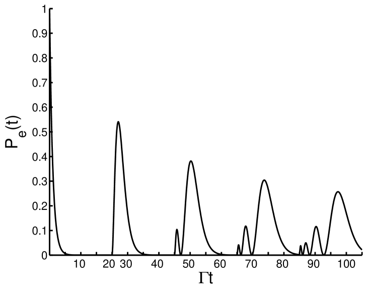
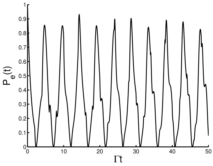
Figure 2: Time dependence of the probability $P_{e}(t)$ of observing the spontaneously decaying two-level system in its excited state at the center of a closed spherical cavity: The number of resonantly interacting field modes is of the order of $\Gamma R/c$ and depends on the size of the cavity $R$. For $\Gamma R/c=10$ (left figure) a spatially localized photon wave packet is generated by spontaneous emission and can be reabsorbed again by the two-level system at the center of the cavity at later times. For $\Gamma R/c=1$ (right figure) only a small number of cavity modes interact resonantly and the two-level system performs approximate Rabi oscillations governed by the vacuum Rabi frequency.

III.2 Spontaneous photon emission in a half-open parabolic cavity

Efficient atom-light interaction in free space Gerhardt ; Sandoghdar ; Tey ; StobAlLeu may provide us with less technologically demanding solutions for quantum communication over large distances than typical cavity quantum electrodynamical solutions CQED . Thus, it has gained a lot of interest recently. An intermediate case between the small-cavity limit and the free-space limit can be realized by a large closed cavity Alber1992 in which an atom couples to a large number of modes and which has been discussed in the previous section. A half-cavity, i.e. a cavity with one mirror, constitutes another example of such a case. The structure of standing light waves in front of a mirror was already analyzed in the pioneering work of K. Drexhage Drexhage1970 . Later on, it has been verified experimentally that under such circumstances one can witness a change of the density of states of the electromagnetic field modes near the atom by measuring its spontaneous emission rate Eschner2001 . A simplified one-dimensional scalar model of a laser-driven atom in a half-cavity has been discussed in Dorner2002 , for example.

As a second example for modifications of the quantum electrodynamical interaction between matter and the radiation field originating from controlled mode engineering in the following we discuss the spontaneous decay of a two-level system, such as an ion Sondermann2007 , in a half-open cavity with a parabolic shape. The two-level system is assumed to be positioned in the focus $F$ of an axially symmetric parabola whose boundary is formed by an ideal metal and is described by the equation $z=\rho^{2}/(4f)$ (compare with Fig.3). The coordinate $z$ measures distances from point $P$ along the symmetry axis and $\rho$ denotes distances perpendicular to the symmetry axis. The focal point $F$ of the parabola has coordinates $(z=f,\rho=0)$ with $f>0$ denoting the focal length. A defining property of any parabola is the fact that the distance between any point on its surface and the focal point $F$ equals the distance to the plane perpendicular to the symmetry axis located at $z=-f$.

We are particularly interested in possible changes of the spontaneous photon emission process of a two-level system resulting from the presence of the parabolic boundary conditions. The parabolic shape of the mirror ensures that, if a light beam is sent parallel to the symmetry axis of the parabola towards the two-level system, this two-level system interacts with the light coming from the whole $4\pi$ solid angle. Similarly, the whole light resulting from spontaneous decay of the two-level system is redirected into a beam propagating parallel to the symmetry axis. Thinking in terms of a semiclassical ray-picture only light rays which are emitted from the two-level system along the (negative part of the) symmetry axis return again to the two-level system. Contrary to the closed spherical cavity discussed in the previous section all other emitted light rays leave the cavity without any reexcitation of the two-level system. Thus, if the dipole moment of the two-level system is oriented along the symmetry axis photon emission along the symmetry axis is suppressed and we do not expect any significant modification of the spontaneous decay process of the two-level system due to the presence of the cavity in cases in which the focal length $f$ is large in comparison with the wavelength of a spontaneously emitted photon Stobinska-Alicki . Nevertheless, in analogy to a small cavity or to spontaneous emission in front of a planar mirror Morawitz1969 significant changes of the spontaneous decay rate are expected if $f$ becomes comparable to the wavelength of a spontaneously emitted photon.

Figure 3: Spontaneous photon emission in a parabolic cavity: The two-level system is positioned in the focus $F$ of a metallic parabola with focal length $f$. All light rays emanating from $F$ which are reflected at the parabolic boundary leave the cavity by propagating parallel to the symmetry axis. They all accumulate the same phase (eikonal) of magnitude $\omega_{eg}(z+f)/c$ which is the same as if these light rays had started in phase from the plane $z=-f$. There are always two possible trajectories to any point ${\bf x}$ inside the cavity. In the semiclassical limit, i.e. $f\gg c/\omega_{eg}$, these two classes of trajectories give rise to the spherical-wave and the plane-wave contributions to the complex-valued energy density amplitude of Eq.(32).

III.2.1 Time evolution of a photon wave packet

First of all, let us consider the dynamics of an almost resonant photon and its resonant energy exchange with a two-level system positioned in the focal point $F$ in the semiclassical limit in which the focal length of the parabola is large in comparison with the photon’s wavelength, i.e. $f\gg c/\omega_{eg}$. Furthermore let us concentrate on cases in which the two-level system’s dipole moment $\langle e|\hat{{\bf d}}|g\rangle$ is oriented parallel to the symmetry axis of the parabola. In particular, we want to investigate solutions of the time dependent Schrödinger equation $|\psi\rangle_{t}$ for which at a certain instant of time, say $t=0$, the two-level system is excited and the electromagnetic radiation field is in its vacuum state, i.e. $|\psi\rangle_{t=0}=|e\rangle\otimes|0\rangle$. Thus, this case describes spontaneous emission of a photon for $t>0$ and perfect excitation of the two-level system by a one-photon field for $t<0$. As $f\gg c/\omega_{eg}$, in the radiation zone, i.e. for $\omega_{eg}|{\bf x}-{\bf x}_{0}|/c\gg 1$, the distribution of the energy density of the electromagnetic field can be determined with the help of semiclassical methods. This is due to the fact that the one-photon energy density amplitudes of the electric and magnetic field energies (compare with Eq.(29)) are rapidly oscillating functions of the radial variable $r=|{\bf x}-{\bf x}_{0}|$ with a slowly varying envelope which decays on the length scale $c/\Gamma$. Stated differently, the condition $\omega_{eg}\gg\Gamma/2$ implies that the phase (eikonal) of these amplitudes exhibits many oscillations within the region of support of these amplitudes.

In the radiation zone the one-photon energy density amplitudes are solutions of the wave equation whose semiclassical solutions Maslov can be constructed with the help of the classical light rays inside the parabolic cavity. Thus, the general form of the energy-density amplitudes of the electric and magnetic field can be constructed semiclassically in two steps. Firstly, one determines their form inside a sphere of radius $R_{0}$ around the focal point $F\equiv{\bf x}_{0}$ so that the condition $c/\omega_{eg}\ll R_{0}\ll f$ is fulfilled. For the electric field this amplitude is given by Eq.(29) and for the magnetic field it can be obtained from Eq.(29) by the replacement ${\bf e}_{\theta}~{}\longrightarrow~{}{\bf e}_{\varphi}$. Semiclassically, with this form of these amplitudes one can associate a Lagrangian manifold Maslov ; Arnold of radially outgoing straight-line trajectories which start at the position of the two-level system $F$ and which propagate with the speed of light. The relevant polarization direction remain constant during transport along these radial trajectories. In a second step one determines the most general semiclassical solution of the wave equation within the parabolic cavity but outside this sphere of radius $R_{0}$. For this purpose one has to construct the light rays outside this sphere thereby taking into account that they are reflected at the boundary of the cavity according to the classical reflection law (equal incoming and outgoing angles). Apart from the reflection process where one has to take into account the boundary conditions of an ideal metal the polarization directions remain constant during the propagation along any of these classical trajectories. The geometry of the parabola implies that after reflection at the metallic boundary the classical trajectories propagate parallel to the symmetry axis. Matching the solutions inside the sphere of radius $R_{0}$ and outside the sphere in a smooth way one obtains the one-photon energy-density amplitude of the electric field at any point ${\bf x}\equiv(z,\rho)$ inside the parabolic cavity. Whereas for times $|t|<f/c$ this energy-density amplitude is given by Eq.(29), for times $t>f/c$ it is modified due to reflections of light rays at the boundary of the parabolic cavity and assumes the form

$${\cal E}({\bf x},t) = -i\sqrt{\frac{3\Gamma\hbar\omega_{eg}}{16\pi c}}\Theta(|t|-r_{1}(z,\rho)/c)e^{i{\rm sgn}(t)\omega_{eg}(|t|-r_{1}(z,\rho)/c)}e^{-\Gamma(|t|-r_{1}(z,\rho)/c)/2}\frac{\sin\left(\theta_{1}(z,\rho)\right)}{r_{1}(z,\rho)}{\bf e}_{\theta_{1}}+$$ (32)

$$-i\sqrt{\frac{3\Gamma\hbar\omega_{eg}}{16\pi c}}\Theta(|t|-\frac{z+f}{c})e^{i{\rm sgn}(t)\omega_{eg}(|t|-(z+f)/c)}e^{-\Gamma(|t|-(z+f)/c)/2}\frac{\sin\left(\theta_{2}(\rho)\right)}{r_{2}(\rho)}{\bf e}_{\rho}$$

with

$$\sin(\theta_{1}(z,\rho))=\frac{\rho}{r_{1}(z,\rho)} r_{1}(z,\rho)=\sqrt{(z-f)^{2}+\rho^{2}}$$ ,

$$\sin(\theta_{2}(\rho))=\frac{\rho}{r_{2}(\rho)} r_{2}(\rho)=f(1+\frac{\rho^{2}}{4f^{2}}).$$ ,

Therefore, at a fixed time $t$ the contribution at position ${\bf x}\equiv(z,\rho)$ results from the interference of contributions originating from radially propagating direct light rays (first term on the r.h.s. of Eq.(32)) with the contributions from light rays reflected at the boundary of the cavity (second term on the r.h.s. of Eq.(32)). Whereas the first type of contributions give rise to a slowly modulated spherical wave front emanating from the position of the two-level system at $F\equiv{\bf x}_{0}$, the reflected trajectories give rise to a (rapidly varying) plane wave propagating in the $z$-direction with a slowly varying amplitude. This plane wave is a consequence of the parabolic geometry of the cavity and the fact that for any point on the boundary of the cavity its distances from the focal point $F$ and from the plane $z=-f$ are equal. Therefore, all light rays emitted at any angle $\theta_{2}$ at $F$ and reflected at the boundary of the parabolic cavity accumulate the same phase (eikonal). This phase is the same as the one originating from a ficticious set of trajectories starting from the plane $z=-f$ and propagating along the $z$-axis with the speed of light. For large focal lengths in the sense that $2f\gg c/\Gamma$ the two contributions to the energy-density amplitude are well separated in space apart from small regions around the boundary of the parabolic cavity. As a consequence interferences between contributions of these two different types of classical trajectories disappear. Furthermore, for a fixed value of $\rho$ the spherical-wave contribution to Eq.(32) becomes vanishingly small in comparison with the plane-wave contribution in the limit of large values of $z$. It is apparent from Eq.(32) that the polarization properties of the spherical-wave contribution are not changed by the cavity and are the same as in free space. However, the polarization features of the plane-wave contribution are significantly different. At any point ${\bf x}$ its polarization is directed in the ${\bf e}_{\rho}$-direction so that the vector field ${\cal E}({\bf x},t)$ represents a vortex field with respect to its polarization properties. The singularity at the symmetry axis is suppressed by the fact that there is not coupling between the radiation field and the two-level system along this axis because the dipole moment of the two-level system is oriented in this direction. Finally, it should be mentioned that the (primitive) semiclassical expression of Eq.(32) breaks down at points close to the boundary of the parabolic cavity where transitional or uniform semiclassical approximations Maslov ; Berry have to be employed.

III.2.2 Modifications of the spontaneous decay rate

In this subsection it will be demonstrated that depending on the characteristic parameters, namely the focal length $f$, the resonant wavelength $\lambda=(2\pi)c/\omega_{eg}$, and the orientation of the two-level system’s dipole moment $d=\langle|\hat{{\bf d}}|g\rangle$, the spontaneous decay rate of the two-level system may differ significantly from its free-space value as given by Eq.(LABEL:spontdec).

Since the two-level system is located in a half-open space we start by expanding the electric field operator (10) in mode functions suitable for the parabolic symmetry of the problem. Following the results of BKM we use mode functions of the form

$${\bf E}^{\sigma}_{k,\ell,\mu}({\bf r})=\frac{k}{(2\pi)^{3/2}}\int_{S^{2}}d{\bf n}\,e^{ik{\bf n}\cdot{\bf r}}\,{h}_{\ell,\mu}({\bf n}){\bf e}^{\sigma}({\bf n}).$$ (33)

Thereby, ${\bf k}=k{\bf n}$ denotes the wavevector, $\sigma=1,2$ enumerates the polarization states, and parameters $\ell=0,\pm 1,\pm 2,...$ and $\mu\in(-\infty,+\infty)$ are additional mode indices. The unit vector ${\bf n}$ and the polarization vectors ${\bf e}^{1}({\bf n}),{\bf e}^{2}({\bf n})$ constitute the orthonormal basis which ensures the transversality condition $\nabla\cdot{\bf E}=0.$ In particular, we choose these directions in the following form

$${\bf n} = (\sin\theta\cos\varphi,\sin\theta\sin\varphi,\cos\theta),$$ (34)

$${\bf e}^{1}({\bf n}) = (\sin\varphi,-\cos\varphi,0),$$ (35)

$${\bf e}^{2}({\bf n}) = (\cos\theta\cos\varphi,\cos\theta\sin\varphi,-\sin\theta).$$ (36)

The functions ${h}_{\ell,\mu}({\bf n})$ are explicitly given by BKM

$$h_{\ell,\mu}(\theta,\varphi)=\chi_{\mu}(\theta)\frac{e^{i\ell\varphi}}{\sqrt{2\pi}},$$ (37)

with

$$\chi_{\mu}(\theta) = \frac{\exp\left(-i\mu\ln[\tan\theta/2]\right)}{\sqrt{2\pi}\sin\theta}.$$ (38)

One can easily check the orthogonality and completeness conditions

$$\int_{0}^{2\pi}\!\!\!\!d\varphi\!\int_{0}^{\pi}\!\!\!d\theta\sin\theta\;h^{*}_{\ell,\mu}(\theta,\varphi)h_{\ell^{\prime},\mu^{\prime}}(\theta,\varphi)=\delta_{\ell\ell^{\prime}}\delta(\mu-\mu^{\prime}),$$ (39)

$$\sum_{\ell=-\infty}^{+\infty}\!\!\int_{-\infty}^{+\infty}\!\!\!d\mu\;h^{*}_{\ell,\mu}(\theta,\varphi)h_{\ell,\mu}(\theta^{\prime},\varphi^{\prime})=\delta(\varphi-\varphi^{\prime})\frac{\delta(\theta-\theta^{\prime})}{\sin\theta}.$$ (40)

Combining Eq. (33) with Eq. (39) one obtains the orthogonality of the mode functions, i.e.

$$\int d{\bf r}\,{\bf E}^{*}{}^{\sigma}_{k,\ell,\mu}({\bf r})\cdot{\bf E}^{\sigma^{\prime}}_{k^{\prime},\ell^{\prime},\mu^{\prime}}({\bf r})=\delta(k-k^{\prime})\delta(\mu-\mu^{\prime})\delta_{\ell\ell^{\prime}}\delta_{\sigma\sigma^{\prime}}.$$ (41)

If a two-level atom is positioned at ${\bf x}$ in free space with the transition dipole parallel to the $z$-axis, in the dipole approximation the resulting spontaneous decay rate is given by

$$\Gamma({\bf x})=\frac{1}{(2\pi)^{2}}\frac{d^{2}k^{3}}{2\hbar\epsilon_{0}}\sum_{\sigma,\ell}\!\int_{-\infty}^{+\infty}\!\!d\mu\int\!d{\bf n}\!\int\!d{\bf n}^{\prime}f_{k}({\bf n},{\bf r})f^{*}_{k}({\bf n}^{\prime},{\bf r})\cdot e^{\sigma}_{z}({\bf n})e^{\sigma}_{z}({\bf n}^{\prime})\,h^{*}_{\ell,\mu}({\bf n},k)h_{\ell,\mu}({\bf n}^{\prime},k)$$ (42)

with $k=\omega_{eg}/c$. Furthermore, we defined $f_{k}({\bf n},{\bf r})={\rm exp}(ik{\bf n}\cdot{\bf r})$, $e^{\sigma}_{z}({\bf n})={\bf e}^{\sigma}({\bf n})\cdot{\bf e}_{z}$, and used the fact that the summation over $\ell$ produces $\delta(\varphi-\varphi^{\prime})$ (see Eq. (40)). Therefore, the relevant directions ${\bf n}$, ${\bf n}^{\prime}$, and the $z$-axis belong to the same plane which leads to the relation

$$\sum_{\sigma}e^{\sigma}_{z}({\bf n})e^{\sigma}_{z}({\bf n}^{\prime})=e^{2}_{z}({\bf n})e^{2}_{z}({\bf n}^{\prime})=\sin\theta\sin\theta^{\prime}.$$ (43)

Taking into account that the integration over $\mu$ yields another Dirac delta distribution $\delta(\theta-\theta^{\prime})$ we finally obtain

$$\Gamma(x,y,z)\!=\!\frac{1}{(2\pi)^{2}}\frac{d^{2}k^{3}}{2\hbar\epsilon_{0}}\int^{2\pi}_{0}\!\!\!d\varphi\!\!\int^{\pi}_{0}\!\!d\theta\sin^{3}\theta|f_{k}(x,y,z;\varphi,\theta)|^{2},$$ (44)

with ${\bf x}\equiv(x,y,z)$ and $f_{k}({\bf n},{\bf r})\equiv f_{k}(x,y,z;\varphi,\theta)$. The relation $|f_{k}(x,y,z;\varphi,\theta)|=1$ implies that we recover again the free-space result of Eq.(LABEL:spontdec).

In the presence of a conducting parabolic mirror the mode functions of Eq. (33) should fulfill the appropriate boundary conditions of an ideal metal. However, it is very challenging to solve the Helmholtz equation under these boundary conditions and the transversality condition simultaneously. Contrary to reference Nockel , a simplified approximation may be obtained by keeping the transversality condition but relaxing the precise conditions on the mode functions on the surface of the parabolic mirror. The transversality condition relates the electric field to the geometry of the system and therefore contributes to some geometrical factor present in the decay rate formula. The boundary condition ensures a possible discreteness of the normal modes. As our physical system is large it is expected that slightly changing the boundary conditions of the parabolic cavity will not influence the decay rate significantly.

We start our approximate treatment by introducing parabolic coordinates $(\xi,\eta,\varphi)$ which are related to Cartesian coordinates by

$$x = 2\sqrt{\xi\eta}\cos\varphi,$$ (45)

$$y = 2\sqrt{\xi\eta}\sin\varphi,$$ (46)

$$z = \xi-\eta.$$ (47)

The boundary of the parabolic mirror is described by the equation $\eta=f$. It can be shown BKM that the important $\eta$-dependent part of the mode functions possesses the following asymptotic behavior

$$F_{\ell,\mu}(k;\eta)\sim\frac{\cos\left\{\mu\ln 2k\eta+k\eta-\alpha_{\ell,\mu}\right\}}{\sqrt{\eta}}$$ (48)

with a phase $\alpha_{\ell,\mu}$ whose explicit form is not important for our subsequent discussion. Imposing the parabolic boundary condition on Eq. (48) at the value $\eta=f$ results in a discrete set of values for $\mu_{m}$. A simple choice for these discrete values is

$$kf-\alpha_{\ell,\mu}=0\ ,\ \mu_{m}\ln 2kf=m\pi\ ,\ m=1,2,3,...$$ (49)

This particular choice is consistent with the replacement of the continuous set of modes of Eq. (38) by the discrete set

$$\tilde{\chi}_{m}(\theta) = \frac{\sin\left(\frac{m\pi\ln[\tan\theta/2]}{\ln 2kf}\right)}{\sqrt{2\pi\ln 2kf}\sin\theta}\;\mathrm{for}\;\theta\in[\theta_{0},\pi-\theta_{0}]$$

$$= 0\ \mathrm{otherwise}$$

such that

$$\tan\frac{\theta_{0}}{2}=\frac{1}{2kf}=\frac{1}{4\pi}\frac{\lambda}{f}.$$ (51)

The limitation on the angle $\theta$ results from the quantization condition (49) and from the fact that at the boundary the normal modes have to vanish, i.e. $\tilde{\chi}_{m}(\theta_{0})=0$. This ansatz modifies the formula for the decay rate because the completeness condition is changed according to

$$\sum_{m}\tilde{\chi}_{m}(\theta)\tilde{\chi}_{m}(\theta^{\prime})=I_{[\theta_{0},\pi-\theta_{0}]}(\theta)\frac{\delta(\theta-\theta^{\prime})}{\sin\theta}$$ (52)

with $I_{A}$ denoting the indicator function of the set $A$. Therefore, the integration over the angle $\theta$ involved in Eq. (42) should be performed over the interval $[\theta_{0},\pi-\theta_{0}]$. This leads to a correction of the order of $(kf)^{-4}$ which, however, is not relevant for present-day experiments. In currently planned experiments Sondermann2007 typical focal lengths and wavelengths are of order of $f=2$mm and $\lambda=250$ nm which amounts to a value of $kf\simeq 10^{4}$ StobAlLeu so that $\theta_{0}$ is small. Therefore, we can replace $\sin\theta$ by $\theta$. It is rather obvious that the same is true for any reasonable choice of the boundary conditions because the smallness of this correction is entirely due to the large value of $kf$.

Hence the only relevant modification of the spontaneous emission rate due to the presence of the parabolic mirror is the replacement of the plane traveling waves $f_{k}({\bf n},{\bf r})=e^{ik{\bf n}\cdot{\bf r}}$ by the standing waves

$$f_{k}({\bf n},{\bf r})=\sqrt{2}\sin\left(k{\bf n}\cdot({\bf r}-{\bf f})\right)$$ (53)

where the factor $\sqrt{2}$ ensures the completeness condition. Eq. (53) implies that the electric field for any mode of the form of Eq. (33) vanishes at the point P of the parabola. It leads to the following approximate expression for the spontaneous emission rate in the presence of a conducting parabolic mirror

$$\tilde{\Gamma}(x,y,z)=\frac{1}{2\pi^{2}}\frac{d^{2}k^{3}}{2\hbar\epsilon_{0}}\int^{2\pi}_{0}\!\!\!d\varphi\int^{\pi}_{0}d\theta\sin^{3}\theta\sin^{2}\{k[(x\cos\varphi+y\sin\varphi)\sin\theta+(z+f)\cos\theta]\}.$$ (54)

If the two-level system is placed at a distance from the point P which is much larger than $\lambda=(2\pi)c/\omega_{eg}$, the interference factor $\sin^{2}(...)$ is averaged to $1/2$ and the standard free-space result of Eq. (LABEL:spontdec) is recovered.

If the two-level system is located at the symmetry axis of the parabola, i.e. $x=y=0$, the integral in Eq. (54) simplifies to

$$\tilde{\Gamma}(z)=\eta\Gamma$$ (55)

with the correction $\eta$ to the free-space decay rate $\Gamma$ being given by

$$\eta=\left(1+3\frac{\cos(2k(z+f))}{4k^{2}(z+f)^{2}}-3\frac{\sin(2k(z+f))}{8k^{3}(z+f)^{3}}\right).$$ (56)

For a focal length $f=2$ mm this correction factor $\eta$ is depicted in Fig. 4. Its value at the focal point $F$ becomes significant for small values of the wave vector $k=c/\omega_{eg}$. This corresponds to cases in which the two-level system is close the mirror surface, i.e. $|z+f|<\lambda$. However, for larger values of $k$ the variations of $\eta$ are shifted towards the mirror surface. Far away from the mirror $\eta$ tends to unity so that the decay rate reduces to its free-space value. According to these results modifications of the spontaneous decay rate could be observable on a scale of $100$nm but only within a distance of the order of the wavelength from the mirror surface.

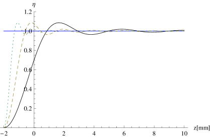
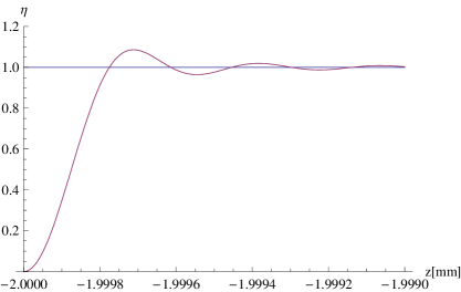
Figure 4: Modifications of the spontaneous decay rate according to Eqs.(55) and (56): small values of $k=(2\pi)c/\omega_{eg}$ (left figure): $k=0.25\pi$ mm^-1 – solid line, $k=0.5\pi$ mm^-1 – dashed line, $k=\pi$ mm^-1 – dotted line; large value of $k=10^{4}$ mm^-1 (right figure).

IV Conclusions and outlook

Despite significant recent advances in the area of cavity quantum electrodynamics concerning the control of photonic quantum states and their interaction with matter in cavities, the interaction of few-photon multi-mode quantum states with matter in free space is still largely unexplored. A detailed understanding of this interaction and the resulting exchange of quantum information between radiation field and matter is not only of general physical interest but is also necessary for promising future quantum technological applications, such as the realization of quantum repeaters.

Here, we have discussed the simplest problem in this respect, namely the free-space interaction of a single-photon quantum state with an individual two-level matter system which can be realized by a trapped atom or ion. In this elementary example it can be demonstrated explicitly that the process of spontaneous emission of a photon is perfectly reversible provided that one is able to control the modes and quantum states of the radiation field in free space. For this purpose the dynamics resulting from the mode structure of a parabolic mirror has been discussed. It has been shown that using parabola it is possible to perfectly convert the excitation of an appropriately prepared asymptotically incoming plane-wave one-photon quantum state to an atom positioned in the focus of the parabola. The resulting dynamics depends strongly on the magnitudes of the dominantly excited wave lengths of the one-photon state. If these wave lengths are short in comparison with the focal length of the parabola the propagation of the one-photon state can be described by semiclassical methods and is dominated by the light rays of the photon inside the parabola. In the opposite limit of long wave lengths diffraction effects become important and semiclassical treatments become inappropriate.

Further experimental testing of the discussed theoretical results is planned. In our future experiment Sondermann2007 ; Maiwald we will use a ${}^{174}\mathrm{Yb}^{2+}$ ion as a two-level system with ${}^{1}S_{0}$ and ${}^{3}P^{0}_{1}$ electronic levels as the ground and the excited state respectively and no hyperfine structure. The atomic transition frequency $\omega_{0}\!\!=\!\!251.8$ nm is in the ultraviolet regime. The ion will be trapped at the focus $f\!=\!2.1$mm of a metallic parabolic mirror, being one electrode of a Paul trap. The rf needle-shaped electrode will come from the back of the mirror through a small hole. This trap design will ensure almost full 4$\pi$ angle of ion-light interaction in the strong focusing regime. The aberration corrections will be done using a diffractive element located in front of the mirror. Since the ion has only one decay channel and its dipole moment will be parallel to the mirror axis we obtain free space geometry. There are several methods which allow for single-photon pulse generation with the desired spatio-temporal shape and spectral distribution. The first relies on electro-optic modulation of a single-photon wave packet Harris . Another experimentally more accessible method applies a strongly attenuated laser pulse containing $\overline{n}\!\!\ll\!\!1$ photons on average. This technique is widely used in Quantum Key Distribution QKD . We can shape a pulsed temporal mode electronically with modulators starting from a continuous-wave laser. Next we will turn it into a radially polarized spatial doughnut mode. After reflection from the mirror surface its polarization, at the focal point will only contribute to polarization parallel to the axis of the mirror and therefore will excite a linear dipole oscillating parallel to this axis. Using this simpler method perfect coupling is achieved if the probability of excitation matches the probability of finding a single photon in the pulse. In addition, as a third option one can generate the properly shaped single-photon Fock state wave function conditionally using photon pairs from parametric down conversion. This method is similar to ghost imaging in the time domain.

Of course, none of these methods will produce an infinitely long pulse. This is not an obstacle for our experiment however, because one can truncate somewhat the exponential tail of the one-photon wavepacket. For example, truncating the pulse to a duration of five lifetimes the excitation probability can be as high as 0.99. For quantum-storage applications it is straightforward to expand this scheme to a lambda transition between two long lived states Pinotsi . Furthermore, efficient coupling in free space opens the possibility for non-linear optics at the single photon level.

The investigations discussed here present first steps towards the future goal of obtaining a detailed understanding of the interaction of individual photons with individual atoms in free space. For future applications in quantum information technology the exploration of the limits of perfect exchange of quantum information between the radiation field and these material systems is of particular interest.

References

- (1) W. Heisenberg: Über quantentheoretische Umdeutung kinematischer und mechanischer Beziehungen, Z. Phys. 33, 879 (1925).
- (2) I. J. R. Aitchison, D. A. MacManus, Th.M.Snyder: Understanding Heisenberg’s ’magical’ paper of July 1925: a new look at the calculational details, arXiv:quant-ph/0404009.
- (3) M. Born and P. Jordan: Zur Quantenmechanik, Z. Phys. 34, 858 (1925).
- (4) E. Schrödinger: Quantisierung als Eigenwertproblem, Ann. Phys. 79, 361 (1926); 79, 489 (1926).
- (5) E. Schrödinger: Über das Verhältnis der Heisenberg-Born-Jordanschen Quantenmechanik zu der meinen, 79, 734 (1926).
- (6) P. A. M. Dirac: The Fundamental Equations of Quantum Mechanics, Proc. Roy. Soc. A 109, 642 (1926).
- (7) V. Weisskopf and E. Wigner: Berechnung der natürlichen Linienbreite aufgrund der Diracschen Lichttheorie, Z. Phys. 63, 54 (1930).
- (8) V. Weisskopf and E. Wigner: Über die natürliche Linienbreite in der Strahlung des harmonischen Oszillators, Z. Phys. 65, 18 (1930).
- (9) Th. Beth and G. Leuchs (eds.), Quantum Information Processing (Wiley-VCH, Weinheim, 2005).
- (10) D. Leibfried, R. Blatt, C. Monroe, and D. Wineland: Quantum Dynamics of Single Trapped Ions, Rev. Mod. Phys. 75, 281 (2003).
- (11) J.Fortagh and C.Zimmermann: Magnetic Microtraps for Ultracold Atoms, Rev. Mod. Phys. 79, 235 (2007).
- (12) C.Winterfeldt, Ch. Spielmann, and G. Gerber: Colloquium: Optimal Control of High-Harmonic Generation, Rev. Mod. Phys. 80, 117 (2008).
- (13) H. Walther, B.T.H. Varcoe, B.G. Englert, T. Becker: Cavity Quantum Electrodynamics, Rep. Prog. Phys. 69, 1325 (2006).
- (14) B.T.H. Varcoe, S. Brattke, M. Weidinger, and H. Walther: Preparing Pure Number States of the Radiation Field, Nature 403, 743 (2000).
- (15) W. P. Schleich, Quantum Optics in Phase Space (Wiley-VCH, Weinheim, 2001).
- (16) S. Quabis, R. Dorn, M. Eberler, O. Gl ckl and G. Leuchs: Focusing light to a tighter spot, Opt. Commun. 179, 1 (2000).
- (17) M. Stobińska, G. Alber, and G. Leuchs: Perfect Excitation of a Matter Qubit by a Single Photon in Free Space, EPL 86, 14007 (2009).
- (18) E. T. Jaynes and F. W. Cummings: Comparison of Quantum and Semiclassical Radiation Theories with Application to the Beam Maser, Proc. IEEE 51, 89 (1963).
- (19) H. Paul: Induzierte Emission bei starker Einstrahlung, Ann. Physik 11, 411 (1963).
- (20) G. Alber: Photon Wave Packets and Spontaneous Decay in a Cavity, Phys. Rev. A 46, R5338 (1992).
- (21) M. Sondermann, R. Maiwald, H. Konermann, N. Lindlein, U. Peschel and G. Leuchs: Design of a Mode Converter for Efficient Light-Atom Coupling in Free Space, App. Phys. B, 89, 489 (2007).
- (22) R. Maiwald, D. Leibfried, J. Britton, J. C. Bergquist, G. Leuchs and D. J. Wineland: Stylus ion trap for enhanced access and sensing, Nature Phys. 5, 551 (2009).
- (23) J. H. Eberly, N. B. Narozhny, and J. J. Sanchez-Mondragon: Periodic Spontaneous Collapse and Revival in a Simple Quantum Model, Phys. Rev. Lett. 44, 1323 (1980).
- (24) I. Sh. Averbukh and N. F. Perel’man: Fractional revivals: Universality in the Long-Term Evolution of Quantum Wave Packets Beyond the Correspondence Principle Dynamics, Phys. Lett. A 139, 449 (1989).
- (25) L. Mandel and E. Wolf, Optical Coherence and Quantum Optics (Cambridge UP, Cambridge, 1995).
- (26) P. Goy, J. M. Raimond, M. Gross, and S. Haroche: Observation of Cavity-Enhanced Single-Atom Spontaneous Emission, Phys. Rev. Lett. 50, 1903 (1983).
- (27) H. A. Bethe: The Electromagnetic Shift of Energy Levels, Phys. Rev. 72, 339 (1947).
- (28) J. Seke: Complete Lamb-shift Calculation to Order by Applying the Methods of Non-Relativistic Quantum Electrodynamics, Nuovo Cimento D 18, 533 (1996).
- (29) J. Seke: Spontaneous Decay of an Unstable Atomic State: New Method for a Unified Nonrelativistic-Relativistic Complete Treatment, Physics Letters A 244, 111 (1998).
- (30) G. Alber and G. M. Nikolopoulos: Quantum Electrodynamics of a Qubit, in Lectures on Quantum Information, edited by D. Bruss and G. Leuchs, p. 555ff (Wiley-VCH, Weinheim, 2007).
- (31) J. D. Jackson, Classical Electrodynamics (Wiley, New York, 1975).
- (32) Handbook of Mathematical Functions, Natl. Bur. Stand. Appl. Math. Ser. No. 55, edited by M. Abramowitz and I. Stegun (U.S. GPO, Washington, D.C., 1964).
- (33) I. Gerhardt, G. Wrigge, P. Bushev, G. Zumofen, M. Agio, R. Pfab, and V. Sandoghdar: Strong Extinction of a Laser Beam by a Single Molecule, Phys. Rev. Lett. 98, 033601 (2007).
- (34) G. Zumofen, N. M. Mojarad, V. Sandoghdar, and M. Agio: Perfect Reflection of Light by an Oscillating Dipole, Phys. Rev. Lett. 101, 180404 (2008).
- (35) M. K. Tey, Z. Chen, S. A. Aljunid, B. Chng, F. Huber, G. Maslennikov, and Ch. Kurtsiefer: Strong Interaction Between Light and a Single Trapped Atom Without the Need for a Cavity, Nature Physics 4, 924 (2008).
- (36) K. H. Drexhage: Monomolecular Layers and Light, Sci. Am. 222, 108 (1970).
- (37) J. Eschner, Ch. Raab, and R. Blatt: Light Interference from Single Atoms and Their Mirror Images, Nature 413, 495 (2001).
- (38) U. Dorner and P. Zoller: Laser-Driven Atoms in Half-Cavities, Phys. Rev. A66, 023816 (2002).
- (39) M. Stobińska and R. Alicki: Single-Photon Single-Ion Interaction in Free Space Configuration in Front of a Parabolic Mirror, arXiv:quant-ph/0905.4014.
- (40) H. Morawitz: Self-Coupling of a Two-Level System by a Mirror, Phys. Rev. 187, 1792 (1969).
- (41) V.P. Maslov and M.V. Fedoriuk, Semi-Classical Approximation in Quantum Mechanics (Reidel, Dordrecht, 1981).
- (42) V. I. Arnold, Mathematical Methods of Classical Mechanics (Springer, Berlin, 1978).
- (43) M. V. Berry and K. E. Mount: Semiclassical Approximations in Wave Mechanics, Rep. Prog. Phys. 35, 315 (1972).
- (44) C. P. Boyer, E. G. Kalnins, and W. Miller: Symmetry and Separation of Variables for the Helmholtz and Laplace Equations, Nagoya Math. J. 60, 35 (1976).
- (45) J. U. Nockel, G. Bourdon, E. Le Ru, R. Adams, I. Robert, J.-M. Moison, and I. Abram: Mode Structure and Ray Dynamics of a Parabolic Dome Microcavity, Phys. Rev. E62, 8677 (2000).
- (46) P. Kolchin, C. Belthangady, S. Du, G. Y. Yin, and S. E. Harris: Electro-Optic Modulation of Single Photons, Phys. Rev. Lett. 101, 103601 (2008).
- (47) N. Gisin, G. Ribordy, W. Tittel, and H. Zbinden: Quantum cryptography, Rev. Mod. Phys. 74, 145 (2002).
- (48) D. Pinotsi and A. Imamoglu: Single Photon Absorption by a Single Quantum Emitter, Phys. Rev. Lett. 100, 093603 (2008).