Testing gaussianity, homogeneity and isotropy with the cosmic microwave background

Abstract

We review the basic hypotheses which motivate the statistical framework used to analyze the cosmic microwave background, and how that framework can be enlarged as we relax those hypotheses. In particular, we try to separate as much as possible the questions of gaussianity, homogeneity and isotropy from each other. We focus both on isotropic estimators of non-gaussianity as well as statistically anisotropic estimators of gaussianity, giving particular emphasis on their signatures and the enhanced “cosmic variances” that become increasingly important as our putative Universe becomes less symmetric. After reviewing the formalism behind some simple model-independent tests, we discuss how these tests can be applied to CMB data when searching for large scale “anomalies”.

1 Introduction

According to our current understanding of the Universe, the morphology of the cosmic microwave background (CMB) temperature field, as well as all cosmological structures that are now visible, like galaxies, clusters of galaxies and the whole web of large-scale structure, are probably the descendants of quantum process that took place some $10^{-35}$ seconds after the Big Bang. In the standard lore, the machinery responsible for these processes is termed cosmic inflation and, in general terms, what it means is that microscopic quantum fluctuations pervading the primordial Universe are stretched to what correspond, today, to cosmological scales (see [1, 2, 3] for comprehensive introductions to inflation.) These primordial perturbations serve as initial conditions for the process of structure formation, which enhance these initial perturbations through gravitational instability. The subsequent (classical) evolution of these instabilities preserves the main statistical features of these fluctuations that were inherited from their inflationary origin – provided, of course, that we restrain ourselves to linear perturbation theory.

However, given that matter has a natural tendency to cluster, and this inevitably leads to non-linearities (not to mention the sorts of complications that come with baryonic physics), the structures which are visible today are far from ideal probes of those statistical properties. CMB photons, on the other hand, to an excellent approximation experience free streaming since the time of decoupling ($z\approx 1100$), and are therefore exempt from these non-linearities (except, of course, for secondary anisotropies such as the Rees-Sciama effect or the Sunyaev-Zel’dovich effect), which implies that they constitute an ideal window to the physics of the early Universe – see, e.g., [4, 5, 6]. In fact, we can determine the primary CMB anisotropies as well as most of the secondary anisotropies on large scales, such as the Integrated Sachs-Wolfe effect, completely in terms of the initial conditions by means of a linear kernel:

$$\Theta(\hat{n})\equiv\frac{\Delta T(\hat{n};\eta_{0})}{T(\eta_{0})}=\int d^{3}x^{\prime}\int_{0}^{\eta_{0}}d\eta^{\prime}\;\sum_{i}K_{i}(\vec{x}\,^{\prime},\eta^{\prime};\hat{n}){\cal{S}}^{i}(\vec{x}\,^{\prime},\eta^{\prime})\;,$$ (1)

where $\eta^{\prime}$ is conformal time, and ${\cal{S}}^{i}$ denote the initial conditions of all matter and metric fields (as well as their time derivatives, if the initial conditions are non-adiabatic.) Here $K_{i}$ is a linear kernel, or a retarded Green’s function, that propagates the radiation field to the time and place of its detection, here on Earth. Since that kernel is insensitive to the statistical nature of the initial conditions (which can be thought of as constants which multiply the source terms), those properties are precisely transferred to the CMB temperature field $\Theta$.

The statistical properties of the primordial fluctuations are, to lowest order in perturbation theory, quite simple: because the quantum fluctuations that get stretched and enhanced by inflation are basically harmonic oscillators in their ground state, the distribution of those fluctuations is Gaussian, with each mode an independent random variable. The Fourier modes of these fluctuations are characterized by random phases (corresponding to the random initial values of the oscillators), with zero mean, and variances which are given simply by the field mass and the mode’s wavenumber $k=2\pi/\lambda$. The presence of higher-order interactions (which exist even for free fields, because of gravity) changes this simple picture, introducing higher-order correlations which destroy gaussianity – even in the simplest scenario of inflation [7, 8, 9]. However, since these interactions are typically suppressed by powers of the factor $GH^{2}\simeq 10^{-12}$, where $G$ is Newton’s constant and $H$ the Hubble parameter during inflation, the corrections are small – but, at least in principle, detectable [10, 11, 12].

Since these statistical properties are a generic prediction of (essentially) all inflationary models, they can also be inferred from two ingredients that are usually assumed as a first approximation to our Universe. First, since inflation was designed to stretch our Universe until it became spatially homogeneous and isotropic, it is reasonable to expect that all statistical momenta of the CMB should be spatially homogeneous and rotationally invariant, regardless of their general form. Second, in linear perturbation theory [13] where we have a large number of cosmological fluctuations evolving independently, we can expect, based on the central limit theorem, that the Universe will obey a Gaussian distribution.

The power of this program lies, therefore, in its simplicity: if the Universe is indeed Gaussian, homogeneous and statistically isotropic (SI), then essentially all the information about inflation and the linear (low redshift) evolution of the Universe is encoded in the variance, or two-point correlation function, of large-scale cosmological structures and/or the CMB. As it turns out, the five year dataset from the Wilkinson Microwave anisotropy probe (WMAP) strongly supports these predictions [14, 11]. Moreover, the measurements of the CMB temperature power spectrum by the WMAP team, alongside measurements of the matter power spectrum from existing survey of galaxies [15, 16] and data from type Ia supernovae [17, 18, 19], have shown remarkable consistency with a concordance model ($\Lambda$CDM), in which the cosmos figures as a Gaussian, spatially flat, approximately homogeneous and statistically isotropic web of structures composed mainly of baryons, dark matter and dark energy.

However, while the detection of a nearly scale-invariant and Gaussian spectrum is a powerful boost to the idea of inflation, just knowing the variance of the primordial fluctuations is not sufficient to single out which particular inflationary model was realized in our Universe. For that we will need not only the 2-point function, but the higher momenta of the distribution as well. Therefore, in order to break this model degeneracy we must go beyond the framework of the $\Lambda$CDM, Gaussian, spatially homogeneous and statistically isotropic Universe.

Reconstructing our cosmic history, however, is not the only reason to explore further the statistical properties of the CMB. The full-sky temperature maps by WMAP [20, 11] have revealed the existence of a series of large-angle anomalies – which, incidentally were (on hindsight) already visible in the lower-resolution COBE data [21]. These anomalies suggest that at least one of our cherished hypothesis underlying the standard cosmological model might be wrong – even as a first-order approximation. Perhaps the most intriguing anomalies (described in more detail in other review papers in this volume) are the low value of the quadrupole and its alignment of the quadrupole ($\ell=2$) with the octupole ($\ell=3$) [22, 23, 24, 25, 26, 27], the sphericity [26] (or lack of planarity [28]), of the multipole $\ell=5$, and the north-south asymmetry [29, 30, 31, 32, 33]. In the framework of the standard cosmological model, these are very unlikely statistical events, and yet the evidence that they exist in the real data (and are not artifacts of poorly subtracted extended foregrounds – e.g., [34]) is strong.

Concerning theoretical explanations, even though we have by now an arsenal of ad-hoc models designed to account for the existence of these anomalies, none has yet quite succeeded in explaining their origin. Nevertheless, they all share the point of view that the detected anomalies might be related to a deviation of gaussianity and/or statistical isotropy.

In this review we will describe, first, how to characterize, from the point of view of the underlying spacetime symmetries, both non-gaussianity and statistical anisotropy. We will adopt two guiding principles. The first is that gaussianity and SI, being completely different properties of a random variable, should be treated separately, whenever possible or practical. Second, since there is only one type of gaussianity and SI but virtually infinite ways away from them, it is important to try to measure these deviations without a particular model or anomaly in mind – although we may eventually appeal to particular models as illustrations or as a means of comparison. This approach is not new and, although not usually mentioned explicitly, it has been adopted in a number of recent papers [35, 36].

One of the main motivations for this model-independent approach is the difficult issue of aprioristic statistics: one can only test the random nature of a process if it can be repeated a very large (formally, infinite) number of times. Since the CMB only changes on a timescale of tens of millions of years, waiting for our surface of last scattering to probe a different region of the Universe is not a practical proposition. Instead, we are stuck with one dataset (a sequence of apparently random numbers), which we can subject to any number of tests. Clearly, by sheer chance about 30% of the tests will give a positive detection with 70% confidence level (C.L.), 10% will give a positive detection with 90% C.L., and so on. With enough time, anyone can come up with detections of arbitrarily high significance – and ingenuity will surely accelerate this process. Hence, it would be useful to have a few guiding principles to inform and motivate our statistical tests, so that we don’t end up shooting blindly at a finite number of fish in a small wheelbarrow.

This review is divided in two parts. We start Part I by reviewing the basic statistical framework behind linear perturbation theory (§2). This serves as a motivation for §3, where we discuss the formal aspects of non-Gaussian and statistically isotropic models (§3.1), as well as Gaussian models of statistical anisotropy (§3.2). Part II is devoted to a discussion on model-independent cosmological tests of non-gaussianity and statistical anisotropy and their application to CMB data. We focus on two particular tests, namely, the multipole vectors statistics (§4) and functional modifications of the two-point correlation function (§5). After discussing how such tests are usually carried out when searching for anomalies in CMB data (§6.1), we present a new formalism which generalizes the standard procedure by including the ergodicity of cosmological data as a possible source of errors (§6.2). This formalism is illustrated in §7, where we carry a search of planar-type deviations of isotropy in CMB data. We then conclude in §8.

Part I The linearized Universe

2 General structure

We start by defining the temperature fluctuation field. Since the background radiation is known to have an average temperature of 2.725K, we are interested only in deviations from this value at a given direction $\hat{n}$ in the CMB sky. So let us consider the dimensionless function on $S^{2}$:

$$\Theta(\hat{n})\equiv\frac{T(\hat{n})-T_{0}}{T_{0}}\;,$$ (2)

where $T_{0}=2.725$ K is the blackbody temperature of the mean photon energy distribution – which, if homogeneity holds, is also equal to the ensemble average of the temperature.

In full generality, the fluctuation field is not only a function of the position vector $\vec{n}$, but also of the time in which our measurements are taken. In practice, the time and displacement of measurements vary so slowly that we can ignore these dependences altogether. Therefore, we can equally well consider this function as one defined only on the unit radius sphere $S^{2}$, for which the following decomposition holds:

$$\Theta(\hat{n})=\sum_{\ell,m}a_{\ell m}Y_{\ell m}(\hat{n})\,.$$ (3)

Since the spherical harmonics $Y_{\ell m}(\hat{n})$ obey the symmetry $Y_{\ell m}^{*}(\hat{n})=(-1)^{m}Y_{\ell,-m}(\hat{n})$, the fact that the temperature field is a real function implies the identity $a_{\ell m}^{*}=(-1)^{m}a_{\ell,-m}$. This means that each temperature multipole $\ell$ is completely characterized by $2\ell+1$ real degrees of freedom.

2.1 From inhomogeneities to anisotropies: linear theory

The ultimate source of anisotropies in the Universe are the inhomogeneities in the baryon-photon fluid, as well as their associated spacetime metric fluctuations. If the photons were in perfect equilibrium with the baryons up to a sharply defined moment in time (the so-called instant recombination approximation), their distribution would have only one parameter (the equilibrium temperature at each point), so that photons flying off in any direction would have exactly the same energies. In that case, the photons we see today coming from a line-of-sight $\hat{n}$ would reflect simply the density and gravitational potentials (the “sources”) at the position $R\,\hat{n}$, where $R$ is the radius to that (instantaneous) last scattering surface. Evidently, multiple scatterings at the epoch of recombination, combined with the fact that anisotropies themselves act as sources for more anisotropies, complicate this picture, and in general the relationship of the sources with the anisotropies must be calculated from either a set of Einstein-Boltzmann equations or, equivalently, from the line-of-sight integral equations coupled with the Einstein, continuity and Euler equations [6].

Assuming for simplicity that recombination was instantaneous, at a time $\eta_{R}$, the linear kernels of Eq. (1) reduce to $K_{i}(\vec{x}\,^{\prime},\eta^{\prime};\hat{n})\rightarrow\beta_{i}\delta(\eta^{\prime}-\eta_{R})\delta(\vec{x}\,^{\prime}-\hat{n}R)$, where $R=\eta_{0}-\eta_{R}$ and $\beta_{i}$ are constant coefficients. The photon distribution that we measure on Earth would therefore be given by:

$$\Theta(\hat{n})\approx\sum_{i}\beta_{i}S^{i}(\vec{x}\,^{\prime}=\hat{n}R,\eta^{\prime}=\eta_{R})\;.$$ (4)

We can also express this result in terms of the Fourier spectrum of the sources:

$$\Theta(\hat{n})\approx\sum_{i}\beta_{i}\int\frac{d^{3}k}{(2\pi)^{3}}e^{i\vec{k}\cdot\hat{n}R}S^{i}(\vec{k},\eta_{R})\;.$$ (5)

Now we can use what is usually referred to as “Rayleigh’s expansion” (though Watson, in his classic book on Bessel functions, attributes this to Bauer, J. f. Math. LVI, 1859):

$$e^{i\vec{k}\cdot\vec{x}}=4\pi\sum_{\ell m}i^{\ell}\,j_{\ell}(kx)\,Y^{*}_{\ell m}(\hat{k})\,Y_{\ell m}(\hat{x})\;,$$ (6)

where $j_{\ell}(z)$ are the spherical Bessel functions. Substituting Eq. (6) into Eq. (5) we obtain that:

$$a_{\ell m}=\int d^{2}\hat{n}\,Y^{*}_{\ell m}(\hat{n})\,\Theta(\hat{n})\approx\int\frac{d^{3}k}{(2\pi)^{3}}\,\Theta(\vec{k})\,\times 4\pi\,i^{\ell}\,j_{\ell}(kR)\,Y_{\ell m}^{*}(\hat{k})\;,$$ (7)

where we have loosely collected the sources into the term $\Theta(\vec{k})\equiv\sum_{i}\beta_{i}S^{i}(\vec{k},\eta_{R})$. This expression conveys well the simple relation between the Fourier modes and the spherical harmonic modes. Therefore, up to coefficients which are known given some background cosmology, the statistical properties of the harmonic coefficients $a_{\ell m}$ are inherited from those of the Fourier modes $\Theta(\vec{k})$ of the underlying matter and metric fields. Notice that the properties of the $a_{\ell m}$’s under rotations, on the other hand, have nothing to do with the statistical properties of the fluctuations: they come directly from the spherical harmonic functions $Y_{\ell m}$.

2.2 Statistics in Fourier space

The characterization of the statistics of random variables is most commonly expressed in terms of the correlation functions. The two-point correlation function is the ensemble expectation value:

$$C(\vec{k},\vec{k}^{\prime})\equiv\langle\Theta(\vec{k})\Theta(\vec{k}^{\prime})\rangle\;.$$ (8)

In the absence of any symmetries, this would be a generic function of the arguments $\vec{k}$ and $\vec{k}^{\prime}$, with only two constraints: first, because $\Theta(\vec{x})$ is a real function, $\Theta^{*}(\vec{k})=\Theta(-\vec{k})$, hence in our definition $C^{*}(\vec{k},\vec{k}^{\prime})=C(-\vec{k},-\vec{k}^{\prime})$; and second, due to the associative nature of the expectation value, $C(\vec{k},\vec{k}^{\prime})=C(\vec{k}^{\prime},\vec{k})$. It is obvious how to generalize this definition to 3, 4 or an arbitrary number of fields at different $\vec{k}$’s (or “points”.)

Let us first discuss the issue of gaussianity. If we say that the variables $\Theta(\vec{k})$ are Gaussian random numbers, then all the information that characterizes their distribution is contained in their two-point function $C(\vec{k},\vec{k}^{\prime})$. The probability distribution function (pdf) is then formally given by:

$$P[\Theta(\vec{k}),\Theta(\vec{k}^{\prime})]\sim\exp\left[-\frac{\Theta(\vec{k})\Theta(\vec{k}^{\prime})}{2\,C(\vec{k},\vec{k}^{\prime})}\right]\;.$$

In this case, all higher-order correlation functions are either zero (for odd numbers of points) or they are simply connected to the two-point function by means of Wick’s Theorem:

$$\langle\Theta(\vec{k}_{1})\Theta(\vec{k}_{2})\ldots\Theta(\vec{k}_{2N})\rangle_{\rm G}=\sum_{i,j}\prod_{\alpha=1}^{N}B_{i,j}^{\alpha}\langle\Theta(\vec{k}_{i})\Theta(\vec{k}_{j})\rangle\;,$$ (9)

where the sum runs over all permutations of the pairs of wave vectors and $B_{i,j}$ are weights.

Second, let’s consider the issue of homogeneity. A field is homogeneous if its expectation values (or averages) do not dependent on the spatial points where they are evaluated. In terms of the $N$-point functions in real space, we should have that:

$$\langle\Theta(\vec{x}_{1})\Theta(\vec{x}_{2})\ldots\Theta(\vec{x}_{N})\rangle\overset{\rm Homog.}{\rightarrow}C_{N}(\vec{x}_{1}-\vec{x}_{2},...,\vec{x}_{N-1}-\vec{x}_{N})\;.$$ (10)

Writing this expression in terms of the Fourier modes, we get that:

$$\langle\Theta(\vec{x}_{1})\Theta(\vec{x}_{2})\ldots\Theta(\vec{x}_{N})\rangle = \int\frac{d^{3}k_{1}\,d^{3}k_{1}\,\ldots d^{3}k_{N}\,}{(2\pi)^{3N}}e^{-i\vec{k}_{1}\cdot\vec{x}_{1}}e^{-i\vec{k}_{2}\cdot\vec{x}_{2}}\ldots e^{-i\vec{k}_{N}\cdot\vec{x}_{N}}$$ (11)

$$\times \langle\Theta(\vec{k}_{1})\Theta(\vec{k}_{2})\ldots\Theta(\vec{k}_{N})\rangle\;.$$

Homogeneity demands that the expression in Eq. (11) is a function of the distances between spatial points only, not of the points themselves. Hence, the expectation value in Fourier space on the right-hand-side of this expression must be proportional to $\delta(\vec{k}_{1}+\vec{k}_{2}+\ldots+\vec{k}_{N})$. In other words, the hypothesis of homogeneity constrains the $N$-point function in Fourier space to be of the form:

$$\langle\Theta(\vec{k}_{1})\Theta(\vec{k}_{2})\ldots\Theta(\vec{k}_{N})\rangle_{\rm H}=(2\pi)^{3}\tilde{N}(\vec{k}_{1},\vec{k}_{2},\ldots,\vec{k}_{N})\,\delta(\vec{k}_{1}+\vec{k}_{2}+\ldots+\vec{k}_{N})\;.$$ (12)

Notice that the “$(N-1)$-spectrum” in Fourier space, $\tilde{N}$, can still be a function of the directions of the wavenumbers $\vec{k}_{i}$ (it will be, in fact, a function of $N-1$ such vectors, due to the global momentum conservation expressed by the $\delta$-function.) Models which realize the general idea of Eq. (12) correspond to homogeneous but anisotropic universes [37, 38, 39, 40].

There is a useful diagrammatic illustration for the $N$-point functions in Fourier space that enforce homogeneity. Notice that we could use the $\delta$-function in Eq. (12) to integrate out any one of the momenta $\vec{k}_{i}$ in Eq. (11). Let us instead rewrite the $\delta$-functions in terms of triangles, so for the 4-point function we have:

$$\delta(\vec{k}_{1}+\vec{k}_{2}+\vec{k}_{3}+\vec{k}_{4})=\int\,d^{3}q\,\delta(\vec{k}_{1}+\vec{k}_{2}-\vec{q})\,\delta(\vec{k}_{3}+\vec{k}_{4}+\vec{q})\;,$$ (13)

whereas for the 5-point function we have:

$$\delta(\vec{k}_{1}+\vec{k}_{2}+\vec{k}_{3}+\vec{k}_{4}+\vec{k}_{5})=\int\,d^{3}q\,d^{3}q^{\prime}\,\delta(\vec{k}_{1}+\vec{k}_{2}-\vec{q})\,\delta(\vec{q}+\vec{k}_{3}-\vec{q}\,^{\prime})\,\delta(\vec{q}\,^{\prime}+\vec{k}_{4}+\vec{k}_{5})\;,$$ (14)

and so on, so that the $N$-point $\delta$-function is reduced to $N-2$ triangles with $N-3$ “internal momenta” (the idea is nicely illustrated in Fig. 1.) Substituting the expression for the $N$-point $\delta$-function into Eq. (11) and integrating out all external momenta but the first ($\vec{k}_{1}$) and last ($\vec{k}_{N}$), the result is that:

$$\langle\Theta(\vec{x}_{1})\Theta(\vec{x}_{2})\ldots\Theta(\vec{x}_{N})\rangle = \frac{1}{(2\pi)^{3N}}\int d^{3}k_{1}\,d^{3}q_{1}\ldots d^{3}q_{N-3}\,d^{3}k_{N}$$ (15)

$$\times e^{i\vec{k}_{1}\cdot(\vec{x}_{1}-\vec{x}_{2})}e^{i\vec{q}_{1}\cdot(\vec{x}_{2}-\vec{x}_{3})}\ldots e^{i\vec{q}_{N-3}\cdot(\vec{x}_{N-2}-\vec{x}_{N-1})}e^{i\vec{k}_{N}\cdot(\vec{x}_{N-1}-\vec{x}_{N})}$$

$$\times \langle\Theta(\vec{k}_{1})\Theta(\vec{q}_{1}-\vec{k}_{1})\ldots\Theta(\vec{k}_{N})\rangle\;.$$

This expressions shows explicitly that the real-space $N$-point function above does not depend on any particular spatial point, only on the intervals between points.

Figure 1: Diagrammatic representation of the 2, 3, 4 and 5-point correlation functions in Fourier space. The dashed lines represent internal momenta.

Finally, what are the constraints imposed on the $N$-point functions that come from isotropy alone? Clearly, no dependence on the directions defined by the points, $\vec{x}_{i}-\vec{x}_{j}$, can arise in the final expression for the $N$-point functions in real space, so from Eq. (11) we see that the $N$-point function in Fourier space should depend only on the moduli of the wavenumbers – up to some momentum-conservation $\delta$-functions, which naturally carry vector degrees of freedom.

In this review we will mostly be concerned with tests of isotropy given homogeneity (but not necessarily Gaussianity), so in our case we will usually assume that the $N$-point function in Fourier space assumes the form given in Eq. (12).

2.3 Statistics in harmonic space

In the previous section we characterized the statistics of our field in Fourier space, which in most cases is most easily related to fundamental models such as inflation. Now we will change to harmonic representation, because that’s what is most directly related to the observations of the CMB, $\Theta(\hat{n})$, which are taken over the unit sphere $S^{2}$. We will discuss mostly the two-point function here, and we defer a fuller discussion of $N$-point functions in harmonic space to Section 3.

From Eq. (7) we can start by taking the two-point function in harmonic space, and computing it in terms of the two-point function in Fourier space:

$$\langle a_{\ell m}a^{*}_{\ell^{\prime}m^{\prime}}\rangle=\int\frac{d^{3}k\,d^{3}k^{\prime}}{(2\pi)^{6}}\,(4\pi)^{2}\,i^{\ell}(-i)^{\ell^{\prime}}\,j_{\ell}(kR)\,j_{\ell^{\prime}}(k^{\prime}R)\,Y_{\ell m}(\hat{k})Y^{*}_{\ell^{\prime}m^{\prime}}(\hat{k}^{\prime})\,\langle\Theta(\vec{k})\Theta^{*}(\vec{k}^{\prime})\rangle\;.$$ (16)

Under the hypothesis of homogeneity, this expression simplifies considerably, leading to:

$$\langle a_{\ell m}a^{*}_{\ell^{\prime}m^{\prime}}\rangle_{\rm H}=\int\,d^{3}k\,\frac{2}{\pi}\,i^{\ell}(-i)^{\ell^{\prime}}\,j_{\ell}(kR)\,j_{\ell^{\prime}}(kR)\,Y_{\ell m}(\hat{k})Y_{\ell^{\prime}m^{\prime}}^{*}(\hat{k})\,\times\,\tilde{N}_{2}(\vec{k})\;.$$ (17)

If, in addition to homogeneity, we also assume isotropy, then $\tilde{N}_{2}\rightarrow P(k)$, and the integration over angles factors out, leading to the orthogonality condition for spherical harmonics:

$$\int\,d^{2}\hat{k}\,Y_{\ell m}(\hat{k})\,Y^{*}_{\ell^{\prime}m^{\prime}}(\hat{k})=\delta_{\ell\ell^{\prime}}\,\delta_{mm^{\prime}}\;,$$

and as a result the covariance of the $a_{\ell m}$’s becomes diagonal:

$$\langle a_{\ell m}a^{*}_{\ell^{\prime}m^{\prime}}\rangle_{\rm H,I} = \delta_{\ell\ell^{\prime}}\,\delta_{mm^{\prime}}\int\,\frac{dk}{k}\,j_{\ell}^{2}(kR)\,\frac{2}{\pi}k^{3}P(k)$$

$$= 4\pi\,\delta_{\ell\ell^{\prime}}\,\delta_{mm^{\prime}}\int\,d\,\log k\,j_{\ell}^{2}(kR)\,\Delta_{T}^{2}(k)$$

$$\equiv C_{\ell}\,\delta_{\ell\ell^{\prime}}\,\delta_{mm^{\prime}}\;,$$

where we have defined the usual temperature power spectrum $\Delta_{T}(k)=k^{3}P(k)/2\pi^{2}$ in the middle line, and the angular power spectrum $C_{\ell}$ in the last line of Eq. (2.3). As a pedagogical note, let’s recall that the power spectrum basically expresses how much power the two-point correlation function has per unit $\log k$:

$$\langle\Theta(\vec{x})\Theta(\vec{x}^{\prime})\rangle_{\rm H,I}=\int d\log k\,\frac{\sin(k|\vec{x}-\vec{x}^{\prime}|)}{k|\vec{x}-\vec{x}^{\prime}|}\,\Delta_{T}^{2}(k)\;.$$ (19)

In an analogous manner to what was done above, we can also construct the angular two-point correlation function in harmonic space:

$$\langle\Theta(\hat{n})\Theta(\hat{n}^{\prime})\rangle = \sum_{\ell m}\sum_{\ell^{\prime}m^{\prime}}\langle a_{\ell m}a^{*}_{\ell^{\prime}m^{\prime}}\rangle Y_{\ell m}(\hat{n})Y^{*}_{\ell m}(\hat{n}^{\prime})\;.$$ (20)

The hypothesis of homogeneity by itself does not lead to significant simplifications, but isotropy leads to a very intuitive expression for the angular two-point function:

$$\langle\Theta(\hat{n})\Theta(\hat{n}^{\prime})\rangle_{\rm H,I} = \sum_{\ell m}\sum_{\ell^{\prime}m^{\prime}}C_{\ell}\,\delta_{\ell\ell^{\prime}}\delta_{mm^{\prime}}Y_{\ell m}(\hat{n})Y^{*}_{\ell m}(\hat{n}^{\prime})$$

$$= \sum_{\ell}C_{\ell}\frac{2\ell+1}{4\pi}P_{\ell}(\hat{n}\cdot\hat{n}^{\prime})\;.$$

Clearly, not only is this expression the analogous in $S^{2}$ of Eq. (19), but in fact the Fourier power spectrum $\Delta_{T}^{2}(k)$ and the angular power spectrum $C_{\ell}$ are defined in terms of each other as indicated in Eq. (2.3):

$$C_{\ell}=4\pi\int d\log k\,j_{\ell}^{2}(kR)\,\Delta_{T}^{2}(k)\;.$$ (22)

Now, using the facts that the spherical Bessel function of order $\ell$ peaks when its argument is approximately given by $\ell$, and that $\int d\log z\,j_{\ell}^{2}(z)=1/(2\ell(\ell+1))$, we obtain that:

$$C_{\ell}\approx\frac{2\pi}{\ell(\ell+1)}\Delta_{T}^{2}(k=\ell/R)\;.$$ (23)

Incidentally, from this expression it is clear why it is customary to define:

$${\cal{C}}_{\ell}\equiv\frac{\ell(\ell+1)}{2\pi}C_{\ell}\approx\Delta_{T}^{2}(k=\ell/R)\;.$$

Using Eq. (11) we can easily generalize the results of this subsection to $N$-point functions in $S^{2}$ and in harmonic space, however, the assumption of isotropy alone does very little to simplify our life. The hypothesis of homogeneity, on the other hand, greatly simplifies the angular $N$-point functions, and most of the work in statistical anisotropy of the CMB that goes beyond the two-point function assumes that homogeneity holds. Notice that the issue of gaussianity is, as always, confined to the question of whether or not the two-point function holds all information about the distribution of the relevant variables, and is therefore completely separated from questions about homogeneity and/or isotropy.

Also notice that the separable nature of the definition (20) implies here as well, like in Fourier space, a reciprocity relation for the correlation function:

$$C(\hat{n}_{1},\hat{n}_{2})=C(\hat{n}_{2},\hat{n}_{1})\,.$$ (24)

This symmetry must hold regardless of underlying models, and is important in order to analyze the symmetries of the correlation function, as we shall see later.

Before we move on, it is perhaps important to mention that the decomposition (20) is not unique. In fact, instead of the angular momenta of the parts, $(\ell_{1},m_{1};\ell_{2},m_{2})$, we could equally well have used the basis of total angular momentum $(L,M;\ell_{1},\ell_{2})$ and decomposed that expression as:

$$C(\hat{n}_{1},\hat{n}_{2})=\sum_{L,M}\sum_{\ell_{1},\ell_{2}}\mathcal{A}_{\ell_{1}\ell_{2}}^{LM}\mathcal{Y}_{\ell_{1}\ell_{2}}^{LM}(\hat{n}_{1},\hat{n}_{2})$$ (25)

where $\mathcal{Y}_{\ell_{1}\ell_{2}}^{LM}$ are known as the bipolar spherical harmonics, defined by [41]:

$$\mathcal{Y}_{\ell_{1}\ell_{2}}^{LM}(\hat{n}_{1},\hat{n}_{2})=[Y_{\ell_{1}}(\hat{n}_{1})\otimes Y_{\ell_{2}}(\hat{n}_{2})]_{LM}\;,$$

where $L$ and $M=m_{1}+m_{2}$ are the eigenvalues of the total and azimuthal angular momentum operators, respectively. This decomposition is completely equivalent to Eq. (20), and we can exchange from one decomposition to another by using the relation:

$$\mathcal{A}_{\ell_{1}\ell_{2}}^{LM}=\sum_{m_{1}m_{2}}\langle a_{\ell_{1}m_{1}}a_{\ell_{2}m_{2}}\rangle(-1)^{M+\ell_{1}-\ell_{2}}\sqrt{2L+1}\left(\begin{array}[]{ccc}\ell_{1}&\ell_{2}&L\\ m_{1}&m_{2}&-M\end{array}\right)\,,$$ (26)

where the $3\times 2$ matrices above are the well-known 3-j coefficients. At this point, it is only a matter of mathematical convenience whether we choose to decompose the correlation function as in (20) or as in (25). Although the bipolar harmonics behave similarly to the usual spherical harmonics in many aspects, the modulations of the correlation function as described in this basis have a peculiar interpretation. We will not go further into detail about this decomposition here, as it is discussed at length in another review article in this volume.

2.4 Estimators and cosmic variance

Returning to the covariance matrix (2.3), we see that, if we assume gaussianity of the $a_{\ell m}$’s, then the angular power spectrum suffices to describe statistically how much the temperature fluctuates in any given angular scale; all we have to do is to calculate the average (2.3). This can be a problem, though, since we have only one Universe to measure, and therefore only one set of $a_{\ell m}$’s. In other words, the average in (2.3) is poorly determined.

At this point, the hypothesis that our Universe is spatially homogeneous and isotropic at cosmological scales comes not only as simplifying assumption about the spacetime symmetries, but also as a remedy to this unavoidable smallness of the working cosmologist’s sample space. If isotropy holds, different cosmological scales are statistically independent, which means that we can take advantage of the ergodic hypothesis and trade averaging over an ensemble for averaging over space. In other words, for a given $\ell$ we can consider each of the $2\ell+1$ real numbers in $a_{\ell m}$ as statistically independent Gaussian random variables, and define a statistical estimator for their variances as the average:

$$\widehat{C}_{\ell}\equiv\frac{1}{2\ell+1}\sum_{m=-\ell}^{\ell}|a_{\ell m}|^{2}\;.$$ (27)

The smaller the angular scales ($\ell$ bigger), the larger the number of independent patches that the CMB sky can be divided into. Therefore, in this limit we should have:

$$\lim_{\ell\rightarrow\infty}\widehat{C}_{\ell}=C_{\ell}\;.$$

On the other hand, for large angular scales (small $\ell$’s), the number of independent patches of our Universe becomes smaller, and (27) becomes a weak estimation of the $C_{\ell}$’s. This means that any statistical analysis of the Universe on large scales will be plagued by this intrinsic cosmic sample variance. Notice that this is an unavoidable limit as long as we have only one observable Universe.

Finally, it is important to keep in mind the clear distinction between the angular power spectrum $C_{\ell}$ and its estimator (27). The former is a theoretical variable which can be calculated from first principles, as we have shown in $\S$2.1. The latter, being a function of the data, is itself a random variable. In fact, if the $a_{\ell m}$’s are Gaussian, then we can rewrite expression (27) as:

$$\frac{(2\ell+1)}{C_{\ell}}\widehat{C}_{\ell}=X_{\ell}\,,\qquad X_{\ell}=\sum_{m=-\ell}^{\ell}\frac{|a_{\ell m}|^{2}}{C_{\ell}}\;,$$

where $X_{\ell}$ is a chi-square random variable with $2\ell+1$ degrees of freedom. According to the central limit theorem, when $\ell\rightarrow\infty$, $X_{\ell}$ approaches a standard normal variable, which implies that $\widehat{C}_{\ell}$ will itself follow a Gaussian distribution. Its mean can be easily calculated using (2.3) and (27), and is of course given by:

$$\langle\widehat{C}_{\ell}\rangle=C_{\ell}\;,$$

which shows that the $\widehat{C}_{\ell}$’s are unbiased estimators of the $C_{\ell}$’s. It is also straightforward to calculate its variance (valid for any $\ell$):

$$\langle(\widehat{C}_{\ell}-C_{\ell})(\widehat{C}_{\ell^{\prime}}-C_{\ell^{\prime}})\rangle=\frac{2}{2\ell+1}\,C_{\ell}^{2}\;\delta_{\ell\ell^{\prime}}\;.$$

Because this estimator does not couple different cosmological scales, it has the minimum cosmic variance we can expect from an estimator due to the finiteness of our sample – so it is optimal in that sense. $\widehat{C}_{\ell}$ is therefore the best estimator we can build to measure the statistical properties of the multipolar coefficients $a_{\ell m}$ when both statistical isotropy and gaussianity hold.

In later Sections we will explore angular or harmonic $N$-point functions for which the assumption of isotropy does not hold. However, it is important to remember at all times that we have only one map, which means one set of $a_{\ell m}$’s. The estimator for the angular power spectrum, $\widehat{C}_{\ell}$, takes into account all the $a_{\ell m}$’s by dividing them into the different $\ell$’s and summing over all $m\in(-\ell,\ell)$. Clearly, it will inherit a sample variance for small $\ell$’s, when the $a_{\ell m}$’s can only be divided into a few “independent parts”. As we try to estimate higher-order objects such as the $N$-point functions, we will have to subdivide the $a_{\ell m}$’s into smaller and smaller subsamples, which are not necessarily independent (in the statistical sense) of each other. So, the price to pay for aiming at higher-order statistics is a worsening of the cosmic sample variance.

2.5 Correlation and statistical independence

The covariance given in Eq. (2.3) has two distinct, important properties. First, note that its diagonal entries, the $C_{\ell}$’s, are $m$-independent coefficients; this is crucial for having statistical isotropy, as we will show latter. Second, statistical isotropy at the Gaussian level implies that different cosmological “scales” (understood here as meaning the modes with total angular momentum $\ell$ and azimuthal momentum $m$) should be statistically independent of each other – and this is represented by the Kronecker deltas in (2.3).

In fact, statistical independence of cosmological scales is a particular property of Gaussian and statistically isotropic random fields, and is not guaranteed to hold when gaussianity is relaxed. We will see in the next Section that the rotationally invariant 3-point correlation function (and in general any $N>2$ correlation function) couples to the three scales involved. In particular, if it happens that the Gaussian contribution of the temperature field is given by (2.3), but at least one of its non-Gaussian moments are nonzero, then the fact that a particular correlation is zero, like for example $\langle a_{2m_{1}}a_{3m_{2}}^{*}\rangle$, does not imply that the scales $\ell=2$ and $\ell=3$ are (statistically) independent. This is just a restatement of the fact that, while statistical independence implies null correlation, the opposite is not necessarily true. This can be illustrated by the following example: consider a random variable $\alpha$ distributed as:

$$P(\alpha)=\begin{cases}1&\alpha\in[0,1]\\ 0&\mbox{otherwise}\,.\end{cases}$$

Let us now define two other variables $x=\cos(2\pi\alpha)$ and $y=\sin(2\pi\alpha)$. From these definitions, it follows that $x$ and $y$ are statistically dependent variables, since knowledge of the mean/variance of $x$ automatically gives the mean/variance of $y$. However, these variables are clearly uncorrelated:

$$\langle xy\rangle=\frac{1}{2\pi}\int_{0}^{2\pi}\cos\eta\sin\eta d\eta=0\,.$$

Although correlations are among cosmologist’s most popular tools when analyzing CMB properties, statistical independence may turn out to be an important property as well, specially at large angular scales, where cosmic variance is more of a critical issue.

3 Beyond the standard statistical model

Until now we have been analyzing the properties of Gaussian and statistically isotropic random temperature fluctuations. This gives us a fairly good statistical description of the Universe in its linear regime, as confirmed by the astonishing success of the $\Lambda$CDM model. This picture is incomplete though, and we have good reasons to search for deviations of either gaussianity and/or statistical isotropy. For example, the observed clustering of matter in galactic environments certainly goes beyond the linear regime where the central limit theorem can be applied, therefore leading to large deviations of gaussianity in the matter power spectrum statistics. Besides, deviations of the cosmological principle may leave an imprint in the statistical moments of cosmological observables, which can be tested by searching for spatial inhomogeneities [42] or directionalities [43].

But how do we plan to go beyond the standard model, given that there is only one Gaussian and statistically isotropic description of the Universe, but infinite possibilities otherwise? This is in fact an ambitious endeavor, which may strongly depend on observational and theoretical hints on the type of signatures we are looking for. In the absence of extra input, it is important to classify these signatures in a general scheme, differentiating those which are non-Gaussian from those which are anisotropic. Furthermore, given that the signatures of non-gaussianity may in principle be quite different from that of statistical anisotropy, such a classification is crucial for data analysis, which requires sophisticated tools capable of separating these two issues.

We therefore start $\S$3.1 by analyzing deviations of gaussianity when statistical isotropy holds. In $\S$3.2 we keep the hypothesis of gaussianity and analyze the consequences of breaking statistical rotational invariance.

3.1 Non-Gaussian and SI models

3.1.1 Rotational invariance of $N$-point correlation functions.

We turn know to the question of non-Gaussian but statistically isotropic probabilities distributions. We will keep working with the $N$-point correlation function defined in harmonic space,

$$\langle a_{\ell_{1}m_{1}}a_{\ell_{2}m_{2}}\dots a_{\ell_{N}m_{N}}\rangle$$ (28)

since knowledge of these functions enables one to fully reconstruct the CMB temperature probability distribution. Specifically, we would like to know the form of any $N$-point correlation function which is invariant under arbitrary 3-dimensional spatial rotations. When rotated to a new (primed) coordinate system, the $N$-point correlation function transforms as:

$$\langle a_{\ell_{1}m^{\prime}_{1}}a_{\ell_{2}m^{\prime}_{2}}\dots a_{\ell_{N}m^{\prime}_{N}}\rangle=\sum_{{\rm all}\,m}\langle a_{\ell_{1}m_{1}}a_{\ell_{2}m_{2}}\dots a_{\ell_{N}m_{N}}\rangle D_{m^{\prime}_{1}m_{1}}^{\ell_{1}}D_{m^{\prime}_{2}m_{2}}^{\ell_{2}}\dots D_{m^{\prime}_{N}m_{N}}^{\ell_{n}}\,,$$ (29)

where the $D_{m_{i}m_{i}^{\prime}}^{\ell}(\alpha,\beta,\gamma)$’s are the coefficients of the Wigner rotation-matrix, which depend on the three Euler-angles $\alpha$, $\beta$ and $\gamma$ characterizing the rotation. Notice that in this notation the primed (rotated) system is indicated by the primed $m$’s. For the 2-point correlation function, we have already seen that the well-known expression

$$\langle a_{\ell_{1}m_{1}}a_{\ell_{2}m_{2}}\rangle=(-1)^{m_{2}}C_{\ell_{1}}\delta_{\ell_{1}\ell_{2}}\delta_{m_{1},-m_{2}}$$

does the job:

$$\langle a_{\ell_{1}m^{\prime}_{1}}a_{\ell_{2}m^{\prime}_{2}}\rangle = C_{\ell_{1}}\left(\sum_{m_{1}}(-1)^{m_{1}}D_{m^{\prime}_{1}m_{1}}^{\ell_{1}}D_{m^{\prime}_{2}-m_{1}}^{\ell_{1}}\right)\delta_{\ell_{1}\ell_{2}}$$

$$= (-1)^{m^{\prime}_{2}}C_{\ell_{1}}\delta_{\ell_{1}\ell_{2}}\delta_{m^{\prime}_{1},-m^{\prime}_{2}}\,.$$

Note the importance of the angular spectrum, $C_{\ell}$, being a $m$-independent function.

What about the 3-point function? In this case, the invariant combination is found to be:

$$\langle a_{\ell_{1}m_{1}}a_{\ell_{2}m_{2}}a_{\ell_{3}m_{3}}\rangle=B_{\ell_{1}\ell_{2}\ell_{3}}\left(\begin{array}[]{ccc}\ell_{1}&\ell_{2}&\ell_{3}\\ m_{1}&m_{2}&m_{3}\end{array}\right)$$

which can be verified by straightforward calculations. Again, the non-trivial physical content of this statistical moment is contained in an arbitrary but otherwise $m$-independent function: the bispectrum $B_{\ell_{1}\ell_{2}\ell_{3}}$ [45, 46, 47]. As we anticipated in Section 2, rotational invariance of the 3-point correlation is not enough to guarantee statistical independence of the three cosmological scales involved in the bispectrum, although in principle a particular model could be formulated to ensure that $B_{\ell_{1}\ell_{2}\ell_{3}}\propto\delta_{\ell_{1}\ell_{2}}\delta_{\ell_{2}\ell_{3}}$, at least for some subset of a general geometric configuration of the 3-point correlation function.

These general properties hold for all the $N$-point correlation function. For the 4-point correlation function, for example, Hu [48] have found the following rotationally invariant combination

$$\langle a_{\ell_{1}m_{1}}\dots a_{\ell_{4}m_{4}}\rangle=\sum_{LM}Q_{\ell_{3}\ell_{4}}^{\ell_{1}\ell_{2}}(L)(-1)^{M}\left(\begin{array}[]{ccc}\ell_{1}&\ell_{2}&L\\ m_{1}&m_{2}&-M\end{array}\right)\left(\begin{array}[]{ccc}\ell_{3}&\ell_{4}&L\\ m_{3}&m_{4}&M\end{array}\right)$$

where the $Q_{\ell_{3}\ell_{4}}^{\ell_{1}\ell_{2}}(L)$ function is known as the trispectrum, and $L$ is an internal angular momentum needed to ensure parity invariance. In a likewise manner, it can be verified that the following expression

$$\langle a_{\ell_{1}m_{1}}\dots a_{\ell_{5}m_{5}}\rangle = \sum_{LM}\sum_{L^{\prime}M^{\prime}}P_{\ell_{3}\ell_{4}\ell_{5}}^{\ell_{1}\ell_{2}}(L,L^{\prime})(-1)^{M+M^{\prime}}\left(\begin{array}[]{ccc}\ell_{1}&\ell_{2}&L\\ m_{1}&m_{2}&-M\end{array}\right)$$

$$\qquad\qquad\times\left(\begin{array}[]{ccc}\ell_{3}&\ell_{4}&L^{\prime}\\ m_{3}&m_{4}&-M^{\prime}\end{array}\right)\left(\begin{array}[]{ccc}\ell_{5}&L&L^{\prime}\\ m_{5}&M&M^{\prime}\end{array}\right)$$

gives the rotationally invariant quadrispectrum $P_{\ell_{3}\ell_{4}\ell_{5}}^{\ell_{1}\ell_{2}}(L,L^{{}^{\prime}})$.

Figure 2: Diagrammatic representation of the 2, 3, 4 and 5-point correlation functions in harmonic space. Here $\vec{\ell}$ actually represents the pair $(\ell,m)$.

The examples above should be enough to show how the general structure of these functions emerges under SI: apart from a $m$-independent function, every pair of momenta $\ell_{i}$ in these functions are connected by a triangle, which in turn connects itself to other triangles through internal momenta when more than 3 scales are present. In Fig. 2 we show some diagrams representing the functions above.

Although we have always shown $N$-point functions which are rotationally invariant, the procedure used for obtaining them was rather intuitive, and therefore does not offer a recipe for constructing general invariant correlation functions. Furthermore, it does not guarantee that this procedure can be extended for arbitrary $N$’s. Here we will present a recipe for doing that, which also guarantees the uniqueness of the solution.

The general recipe for obtaining the rotationally invariant $N$-point function is as follows: from the expression (29) above, we start by contracting every pairs of Wigner functions, where by “contracting” we mean using the identity

$$D_{m^{\prime}_{1}m_{1}}^{\ell_{1}}(\omega)D_{m^{\prime}_{2}m_{2}}^{\ell_{2}}(\omega) = \sum_{L,M,M^{\prime}}\left(\begin{array}[]{ccc}\ell_{1}&\ell_{2}&L\\ m^{\prime}_{1}&m^{\prime}_{2}&-M\end{array}\right)\left(\begin{array}[]{ccc}\ell_{1}&\ell_{2}&L\\ m_{1}&m_{2}&-M^{\prime}\end{array}\right)$$

$$\times(2L+1)(-1)^{M+M^{\prime}}D_{M^{\prime}M}^{L}(\omega)$$

and where $\omega=\{\alpha,\beta,\gamma\}$ is a shortcut notation for the three Euler angles. Once this contraction is done there will remain $\lceil N/2\rceil$ $D$-functions, which can again be contracted in pairs. This procedure should be repeated until there is only one Wigner function left, in which case we will have an expression of the following form:

$$\langle a_{\ell_{1}m_{1}}\dots a_{\ell_{N}m_{N}}\rangle=\sum_{{\rm all}\,m^{\prime}}\langle a_{\ell_{1}m^{\prime}_{1}}\dots a_{\ell_{N}m^{\prime}_{N}}\rangle\times\sum\mbox{geometrical factors}\times D_{MM^{\prime}}^{L}(\omega)\,.$$

Now, we see that the only way for this combination to be rotationally invariant is when the remaining $D_{MM^{\prime}}^{L}$ function above does not depend on $\omega$, i.e., $D_{MM^{\prime}}^{L}(\omega)=\delta_{L0}\delta_{M0}\delta_{M^{\prime}0}$. Once this identity is applied to the geometrical factors, we are done, and the remaining terms inside the primed $m$-summation will give the rotationally invariant ($N$-1)-spectrum.

As an illustration of this algorithm, let us construct the rotationally invariant spectrum and bispectrum. For the 2-point function there is only one contraction to be done, and after we simplify the last Wigner function we arrive at

$$\langle a_{\ell_{1}m_{1}}a_{\ell_{2}m_{2}}\rangle=\left[\sum_{m^{\prime}_{1}}\frac{\langle|a_{\ell_{1}m^{\prime}_{1}}|^{2}\rangle}{2\ell_{1}+1}\right](-1)^{m_{2}}\delta_{\ell_{1}\ell_{2}}\delta_{m_{1},-m_{2}}\;,$$

where, of course:

$$C_{\ell}\equiv\frac{1}{2\ell+1}\sum_{m}\langle|a_{\ell m}|^{2}\rangle\;,$$

is the well-known definition of the temperature angular spectrum. For the 3-point function there are two contractions, and the simplification of the last Wigner function gives

$$\langle a_{\ell_{1}m_{1}}a_{\ell_{2}m_{2}}a_{\ell_{3}m_{3}}\rangle=\left[\sum_{m^{\prime}_{1},m^{\prime}_{2},m^{\prime}_{3}}\langle a_{\ell_{1}m^{\prime}_{1}}a_{\ell_{2}m^{\prime}_{2}}a_{\ell_{3}m^{\prime}_{3}}\rangle\left(\begin{array}[]{ccc}\ell_{1}&\ell_{2}&\ell_{3}\\ m^{\prime}_{1}&m^{\prime}_{2}&m^{\prime}_{3}\end{array}\right)\right]\left(\begin{array}[]{ccc}\ell_{1}&\ell_{2}&\ell_{3}\\ m_{1}&m_{2}&m_{3}\end{array}\right)\,.$$

From this expression and the ortoghonality of the 3-j’s symbols (see the Appendix), we can immediately identify the definition of the bispectrum:

$$B_{\ell_{1}\ell_{2}\ell_{3}}\equiv\sum_{m_{1},m_{2},m_{3}}\langle a_{\ell_{1}m_{1}}a_{\ell_{2}m_{2}}a_{\ell_{3}m_{3}}\rangle\left(\begin{array}[]{ccc}\ell_{1}&\ell_{2}&\ell_{3}\\ m_{1}&m_{2}&m_{3}\end{array}\right)\,.$$

It should be mentioned that this recipe not only enables us to establish the rotational invariance of any $N$-point correlation function, but it also furnishes a straightforward definition of unbiased estimators for the $N$-point functions. All we have to do is to drop the ensemble average of the primed $a_{\ell m}$’s. So, for example, for the 2- and 3-point functions above, the unbiased estimators are given respectively by:

$$\widehat{C}_{\ell} = \frac{1}{2\ell+1}\sum_{m}a_{\ell m}a_{\ell m}^{*}$$

$$\widehat{B}_{\ell_{1}\ell_{2}\ell_{3}} = \sum_{m_{1},m_{2},m_{3}}a_{\ell_{1}m_{1}}a_{\ell_{2}m_{2}}a_{\ell_{3}m_{3}}\left(\begin{array}[]{ccc}\ell_{1}&\ell_{2}&\ell_{3}\\ m_{1}&m_{2}&m_{3}\end{array}\right)\,.$$

Notice that isotropy plays the same role, in $S^{2}$, that homogeneity plays in $\mathbb{R}^{3}$. What enforces homogeneity in $\mathbb{R}^{3}$ is the Fourier-space $\delta$-functions, as in the discussion around Fig. 1. However, in $S^{2}$ the equivalent of the Fourier modes are the harmonic modes, for which there is only a discrete notion of orthogonality – and no Dirac $\delta$-function. What we found above is that the Wigner 3-j symbols play the same role as the Fourier space $\delta$-functions: they are the enforcers of isotropy (rotational invariance) for the $N$-point angular correlation function. Hence, the diagrammatic representations of the constituents of the $N$-point functions in Fourier (Fig. 1) and in harmonic space (Fig. 2) really do convey the same physical idea – one in $\mathbb{R}^{3}$, the other in $S^{2}$.

3.2 Gaussian and Statistically Anisotropic models

In the last section, we have developed an algorithm which enables one to establish the rotational invariance of any $N$-point correlation function. As we have shown, this is also an algorithm for building unbiased estimators of non-Gaussian correlations. In this section we will change the perspective and analyze the case of Gaussian but statistically anisotropic models of the Universe.

There are many ways in which statistical anisotropy may be manifested in CMB. From a fundamental perspective, a short phase of inflation which produces just enough e-folds to solve the standard Big Bang problems may leave imprints on the largest scales of the Universe, provided that the spacetime is sufficiently anisotropic at the onset of inflation [39]. Another source of anisotropy may result from our inability to efficiently clean foreground contaminations from temperature maps. Usually, the cleaning procedure involves the application of a mask function in order to eliminate contaminations of the galactic plane from raw data. As a consequence, this procedure may either induce, as well as hide some anomalies in CMB maps [28].

It is important to mention that these two examples can be perfectly treated as Gaussian: in the first case, the anisotropy of the spacetime can be established in the linear regime of perturbation theory, and therefore will not destroy gaussianity of the quantum modes, provided that they are initially Gaussian. In the second case, the mask acts linearly over the temperature maps, therefore preserving its probability distribution [49].

3.2.1 Primordial anisotropy

Recently, there have been many attempts to test the isotropy of the primordial Universe through the signatures of an anisotropic inflationary phase [38, 39, 40, 50, 51]. A generic prediction of such models is the linear coupling of the scalar, vector and tensor modes through the spatial shear, which is in turn induced by anisotropy of the spacetime [38]. Whenever that happens, the matter power spectrum, defined in a similar way as in Eq. (12), will acquire a directionality dependence due to this type of see-saw mechanism. This dependence can be accommodated in a harmonic expansion of the form:

$$P(\vec{k})=\sum_{\ell,m}r_{\ell m}(k)Y_{\ell m}(\hat{k})\;,$$ (34)

where the reality of $P(\vec{k})$ requires that $r_{\ell m}(k)=(-1)^{m}r_{\ell,-m}^{*}(k)$. Given that temperature perturbations $\Theta(\vec{x})$ are real, their Fourier components must satisfy the relation $\Theta(\vec{k})=\Theta^{*}(-\vec{k})$. This property taken together with the definition (12) implies that:

$$P(\vec{k})=P(-\vec{k})\;,$$ (35)

which in turn restricts the $\ell$’s in (34) to even values. Also, note that by relaxing the assumption of spatial isotropy, we are only breaking a continuous spacetime symmetry, but discrete symmetries such as parity should still be present in this class of models. Indeed, by imposing invariance of the spectrum under the transformation $z\rightarrow-z$, we find that $(-1)^{\ell-m}=1$. Similarly, invariance under the transformations $x\rightarrow-x$ and $y\rightarrow-y$ imply the conditions $r_{\ell m}=(-1)^{m}r_{\ell,-m}$ and $r_{\ell m}=r_{\ell,-m}$, respectively. Gathering all these constraints with the parity of $\ell$, we conclude that

$$r_{\ell m}\in\mathbb{R},\qquad\ell,m\in 2\mathbb{N}\,.$$ (36)

That is, from the initial $2\ell+1$ degrees of freedom, only $\ell/2+1$ of them contribute to the anisotropic spectrum [39].

3.2.2 Signatures of statistical anisotropies

The selection rules (36) are the most generic predictions we can expect from models with global break of anisotropy. We will now work out the consequences of these rules to the temperature power spectrum, and check whether they can say something about the CMB large scale anomalies.

From the expressions (16) and (34) we can immediately calculate the most general anisotropic covariance matrix [37]:

$$\langle a_{\ell_{1}m_{1}}a_{\ell_{2}m_{2}}^{*}\rangle=\sum_{\ell_{3},m_{3}}\mathcal{G}_{m_{1}m_{2}m_{3}}^{\ell_{1}\ell_{2}\ell_{3}}H_{\ell_{1}\ell_{2}}^{\ell_{3}m_{3}}\;,$$ (37)

where:

$$\mathcal{G}_{m_{1}m_{2}m_{3}}^{\ell_{1}\ell_{2}\ell_{3}}=(-1)^{m_{1}}\sqrt{\frac{(2\ell_{1}+1)(2\ell_{2}+1)(2\ell_{3}+1)}{4\pi}}\left(\begin{array}[]{ccc}\ell_{1}&\ell_{2}&\ell_{3}\\ 0&0&0\end{array}\right)\left(\begin{array}[]{ccc}\ell_{1}&\ell_{2}&\ell_{3}\\ -m_{1}&m_{2}&m_{3}\end{array}\right)\,,$$ (38)

are the Gaunt coefficients resulting from the integral of three spherical harmonics (see the Appendix). These coefficients are zero unless the following conditions are met:

$$\begin{cases}\ell_{1}+\ell_{2}+\ell_{3}&\in 2\mathbb{N}\\ m_{1}+m_{2}+m_{3}&=0\\ |\ell_{i}-\ell_{j}|\leq\ell_{k}\leq\ell_{i}+\ell_{j}&\forall i,j,k\in\{1,2,3\}\;.\end{cases}$$ (39)

The remaining coefficients in (37) are given by:

$$H_{\ell_{1}\ell_{2}}^{\ell_{3}m_{3}}=4\pi i^{\ell_{1}-\ell_{2}}\int_{0}^{\infty}{d\log k}\;r_{\ell_{3}m_{3}}(k)j_{\ell_{1}}(kR)j_{\ell_{2}}(kR)\,,$$

and correspond to the anisotropic generalization of temperature power spectrum (2.3).

The selection rules (39), taken together with (36), lead to important signatures in the CMB. In particular, since $\ell_{3}$ is even, the quantity $\ell_{1}\pm\ell_{2}$ must also be even, i.e., multipoles with different parity do not couple to each other in this class of models:

$$\langle a_{\ell_{1}m_{1}}a_{\ell_{2}m_{2}}^{*}\rangle=0\,,\qquad\ell_{1}+\ell_{2}=\mbox{odd}\,.$$ (40)

This result is in fact expected on theoretical grounds, because by breaking a continuous symmetry (isotropy) we cannot expect to generate a discrete signature (parity) in CMB. However, notice that the absence of correlations between, say, the quadrupole and the octupole, does not imply that there will be no alignment between them. One example of this would be a covariance matrix of the form $C_{\ell m}\delta_{\ell\ell^{\prime}}\delta_{mm^{\prime}}$. If the $C_{\ell,0}$ happen to be zero, for example, then all multipoles will present a preferred direction (in this case, the $z$-axis.)

3.2.3 Isotropic signature of statistical anisotropy

We have just shown that a generic consequence of an early anisotropic phase of the Universe is the generation of even-parity signatures in CMB maps. Interestingly, these signatures may be present even in the isotropic angular spectrum, since the $C_{\ell}$’s acquire some additional modulations in the presence of statistical anisotropies. In principle, these modulations could be constrained by measuring an effective angular spectrum of the form

$$\langle a_{\ell m}a_{\ell m}^{*}\rangle=C_{\ell}+\epsilon\sum_{\ell^{\prime}>0}\mathcal{G}_{m,-m,0}^{\ell\ell\ell^{\prime}}H_{\ell\ell}^{\ell^{\prime}0}\;,$$ (41)

where we have introduced a small $\epsilon$ parameter to quantify the amount of primordial anisotropy.

In order to constrain these modulations we have to build a statistical estimator for $\langle a_{\ell m}a_{\ell m}^{*}\rangle$. Since we are looking for the diagonal entries of the matrix (37), a first guess would be

$$\widehat{C}_{\ell}^{{\rm eff}}=\frac{1}{2\ell+1}\sum_{m=-\ell}^{\ell}a_{\ell m}a_{\ell m}^{*}\,.$$ (42)

To check whether this is an unbiased estimator of the effective angular spectrum, we apply it to (37) and take its average:

$$\langle C_{\ell}^{{\rm eff}}\rangle=C_{\ell}+\epsilon\sum_{\ell^{\prime}>0,m}\mathcal{G}_{m,-m,0}^{\ell\ell\ell^{\prime}}H_{\ell\ell}^{\ell^{\prime}0}\,.$$

Using the definition (38) of the Gaunt coefficients, the $m$-summation in the expression above becomes [41]

$$\sum_{m}(-1)^{\ell-m}\left(\begin{array}[]{ccc}\ell&\ell&\ell^{\prime}\\ m&-m&0\end{array}\right)=\sqrt{2\ell+1}\delta_{\ell^{\prime},0}=0$$

where the last equality follows because $\ell^{\prime}>0$. Consequently we conclude that

$$\langle\widehat{C}_{\ell}^{{\rm eff}}\rangle=C_{\ell}\neq\langle a_{\ell m}a_{\ell m}^{*}\rangle\,.$$

At first sight, this result may seem innocuous, showing only that this is not an appropriate estimator for (41). Note however that (42) is in fact the estimator of the angular spectrum usually applied to CMB data under the assumption of statistical isotropy. In other words, by means of the usual procedure we may be neglecting important information about statistical anisotropy. Moreover, the cosmic variance induced by the application of this estimator on anisotropic CMB maps is small, because, as it can easily be checked:

$$\langle(\widehat{C}_{\ell}^{{\rm eff}}-C_{\ell})(\widehat{C}_{\ell^{\prime}}^{{\rm eff}}-C_{\ell^{\prime}})\rangle=\frac{2}{2\ell+1}\,C_{\ell}^{2}\,\delta_{\ell\ell^{\prime}}+\mathcal{O}(\epsilon^{2})\;.$$

This result shows that the construction of statistical estimators strongly depends on our prejudices about what non-gaussianity and statistical anisotropy should look like. Consequently, an estimator built to measure one particular property of the CMB may equally well hide other important signatures. One possible solution to this problem is to let the construction of our estimators be based on what the observations seem to tell us, as we will do in the next Section.

Part II Cosmological Tests

So much for mathematical formalism. We will now turn to the question of how the hypotheses of gaussianity and statistical isotropy of the Universe can be tested. Though we are primarily interested in applying these tests to CMB temperature maps, most of the tools we shall be dealing with can be applied to polarization ($E$- and $B$-mode maps) and to catalogs of large-scale structures as well.

Testing the gaussianity and SI of our Universe is a difficult task. Specially because, as we have seen, there is only one Gaussian and SI Universe, but infinitely many universes which are neither Gaussian nor isotropic. So what type of non-gaussianity and statistical anisotropy should we test for? In order to attack this problem we can follow two different routes. In the bottom-up approach, models for the cosmic evolution are formulated in such a way as to account for some specific deviations from gaussianity and SI. These physical principles range from non-trivial cosmic topologies [52, 53, 54], primordial magnetic fields [55, 56, 57, 58, 59], local [60, 43, 61, 62] and global [38, 39, 40, 50] manifestation of anisotropy, to non-minimal inflationary models [51, 63, 64, 65, 66, 67]. The main advantage of the bottom-up approach is that we know exactly what feature of the CMB is being measured. One of its drawbacks is the plethora of different models and mechanisms that can be tested.

The second possibility is the top-down, or model-independent approach. Here, we are not concerned with the mechanisms responsible for deviations of gaussianity or SI, but rather with the qualitative features of any such deviation. Once these features are understood, we can use them as a guide for model building. Examples here include constructs of a posteriori statistics [29, 35, 36] and functional modifications of the two-point correlation function [28, 37, 68, 69, 70, 71].

In the next section we will explore two different model-independent tests: one based on functional modifications of the two-point correlation function, and another one based on the so-called Maxwell’s multipole vectors.

4 Multipole vectors

Multipole vectors were first introduced in cosmology by Copi et al. [23] as a new mathematical representation for the primordial temperature field, where each of its multipoles $\ell$ are represented by $\ell$ unit real vectors. Later it was realized that this idea is in fact much older [72], being proposed originally by J. C. Maxwell in his Treatise on Electricity and Magnetism.

The power of this approach is that the multipole vectors can be entirely calculated in terms of a temperature map, without any reference to external reference frames. This make them ideal tools to test the morphology of CMB maps, like the quadrupole-octupole alignment.

The purpose of the following presentation is only comprehensiveness. A mathematically rigorous introduction to the subject can be found in references [73, 72, 74], as well as other review articles in this review volume.

4.1 Maxwell’s representation of harmonic functions

We start our presentation of the multipole vectors by recalling some terminology. A harmonic function in three dimensions is any (twice differentiable) function $h$ that satisfies Laplace’s equation:

$$\nabla^{2}h=0\;,$$ (43)

where $\nabla^{2}$ is the Laplace operator. In spherical coordinates, the formal solution to Laplace’s equation which is regular at the origin ($r=0$) is:

$$h=\sum_{\ell=0}^{\infty}h_{\ell}(r,\theta,\varphi)\,,\qquad h_{\ell}=\sum_{m=-\ell}^{\ell}a_{\ell m}r^{\ell}Y_{\ell m}(\theta,\varphi)\,.$$ (44)

The functions $r^{\ell}Y_{\ell m}$ are known as the solid spherical harmonics [74]. Since they agree with the usual spherical harmonics on the unit sphere, it is sometimes stated in the literature that the latter form a set of harmonic functions. This is an abuse of nomenclature though, and the reader should be careful.

Given the scalar nature of Laplace’s operator, it is possible to find solutions to Eq.(43) in terms of Cartesian coordinates. Such solutions can be constructed by combining homogeneous polynomials of order $\ell$:

$$h=\sum_{\ell=0}^{\infty}h_{\ell}(x,y,z)\,,\quad h_{\ell}=\sum_{abc}^{\ell}\lambda_{abc}x^{a}y^{b}z^{c}\,,\quad(a+b+c=\ell)\,.$$ (45)

In three dimensions, the most general homogeneous polynomial of order $\ell$ contains $(\ell+2)!/(2!\ell!)$ independent coefficients. However, since each polynomial must independently satisfy Eq. (43), precisely $\ell!/(2!(\ell-2)!)$ of these coefficients will depend on each other. This constraint leaves us with $(\ell+1)(\ell+2)/2-\ell(\ell-1)/2=2\ell+1$ independent degrees of freedom in each multipole $\ell$ – which is, of course, the same number of independent degrees of freedom appearing in Eq. (44).

Based on this analysis, Maxwell introduced his own representation of harmonic functions. He noticed that by successively applying directional derivatives of the form $\vec{v}\cdot\nabla\equiv\nabla_{\vec{v}}$ over the monopole potential $1/r$, where $r=\sqrt{x^{2}+y^{2}+z^{2}}$ and $\vec{v}$ is a unit vector, he could construct solutions of the form (45). That is:

$$f_{\ell}(x,y,z)=\lambda_{\ell}\left.\nabla_{\vec{v}_{\ell}}\dots\nabla_{\vec{v}_{2}}\nabla_{\vec{v}_{1}}\frac{1}{r}\right|_{r=1}\;,$$ (46)

where $\lambda_{\ell}$ are real constants. We are now going to show that this construction does indeed lead to solutions of the form (45). First, note that there is a pattern which emerges from successive application of directional derivatives over the monopole function:

$$f_{0} = \frac{1}{r}$$

$$f_{1} = \nabla_{\vec{v}_{1}}f_{0}=\frac{-\vec{v}_{1}\cdot\vec{r}}{r^{3}}$$

$$f_{2} = \nabla_{\vec{v}_{2}}f_{1}=\frac{3(\vec{v}_{2}\cdot\vec{r})(\vec{v}_{1}\cdot\vec{r})-r^{2}(\vec{v}_{1}\cdot\vec{v}_{2})}{r^{3}}\;,$$ (47)

and so on. By induction, one can show that the general expression will be given by:

$$f_{\ell}=\frac{(-1)^{\ell}(2\ell-1)!!\prod_{i=1}^{\ell}\vec{v}_{i}\cdot\vec{r}+r^{2}Q_{\ell-2}}{r^{2\ell+1}}\,,$$ (48)

where $Q_{\ell-2}$ is a homogeneous polynomial of order $\ell-2$ which only involves combinations of the vectors $\vec{v}_{i}$ and $\vec{r}$.

The numerator of the function $f_{\ell}$ given by (48) is clearly a homogeneous polynomial of order $\ell$ (as one can easily check for some $\ell$’s and also prove by mathematical induction.) A not so obvious result is that this polynomial is also harmonic. To prove that, let us define:

$$g_{\ell}=(-1)^{\ell}(2\ell-1)!!\prod_{i=1}^{\ell}\vec{v}_{i}\cdot\vec{r}+r^{2}Q_{\ell-2}\,,$$ (49)

and consider the application of the operator $\nabla^{2}$ over the combination $r^{\alpha}g_{\ell}$. For the $x$-component we get:

$$\partial_{x}^{2}(r^{\alpha}g_{\ell})=r^{\alpha}\partial_{x}^{2}g_{\ell}+2\alpha r^{\alpha-2}x\partial_{x}g_{\ell}+[\alpha r^{\alpha-2}+\alpha(\alpha-2)x^{2}r^{\alpha-4}]g_{\ell}\,.$$

Repeating this process for the $y$- and $z$-components and then adding the results, we find:

$$\nabla^{2}(r^{\alpha}g_{\ell}) = r^{\alpha}\nabla^{2}g_{\ell}+2\alpha r^{\alpha-2}(x\partial_{x}g_{\ell}+y\partial_{y}g_{\ell}+z\partial_{z}g_{\ell})+\alpha(\alpha+1)r^{\alpha-2}g_{\ell}$$

$$= r^{\alpha}\nabla^{2}g_{\ell}+\alpha(\alpha+2\ell+1)(r^{\alpha-2}g_{\ell})\,,$$

where in the last step we have used Euler’s theorem on homogeneous functions, i.e., $\vec{r}\cdot\nabla g_{\ell}=\ell g_{\ell}$. If we now choose $\alpha=-(2\ell+1)$, we find immediately that

$$\nabla^{2}\left(\frac{g_{\ell}}{r^{2\ell+1}}\right)=\frac{\nabla^{2}g_{\ell}}{r^{2\ell+1}}\,.$$

By construction, the left-hand side of the above expression is equal to $\nabla^{2}f_{\ell}$. But according to the definition (46) this quantity is also zero, since Laplace’s operator commutes with directional derivatives and $\nabla^{2}(1/r)=0$ for $r>0$. Therefore, $\nabla^{2}g_{\ell}=0$ and $g_{\ell}$ is harmonic, which completes our proof.

In conclusion, Maxwell’s construction of harmonic functions, Eq. (46), is completely equivalent to the standard representation in terms of spherical harmonics. More importantly, this gives a one-to-one relationship between temperature maps (given by the $a_{\ell m}$’s) and $\ell$ unit vectors $\vec{v}_{i}$. This means that the multipole vectors can be directly calculated from a CMB map, without any reference to external reference frames or additional geometrical constructs. The reader interested in algorithms to construct the vectors from CMB maps may check references [23, 72], as well as the other articles in this volume that review this approach.

4.2 Multipole vectors statistics

It should be clear from the discussion above that the multipole vectors give an intuitive way to discover, interpret and visualize phase correlations between different multipoles in the CMB maps. But they also can reveal intra-multipole features, such as planarity (when a given multipole presents a preferred plane.) Some of the most conspicuous hints of statistical anisotropy in the CMB, like the quadrupole-octupole alignment, have indeed been first found with less mathematically elegant methods [22, 27], but are best described in terms of the multipole vector formalism [23, 24, 26, 72]. However, this case should also sound an alarm, because some feature of a (presumably) random realization was found, then further scrutinized with a certain test which was, to some extent (intentionally or not) tailored to single out that very feature.

The pitfalls of aprioristic approaches are sometimes unavoidable, and all we can do is take a second look at our sample with a more generic set of tools, to try to assess how significant our result really is in the context of a larger set of statistical tests. Multipole vectors are, in fact, ideally suited to this, since they can be found for all multipoles, and it is relatively easy to construct scalar combinations of these vectors with the usual methods of linear algebra. Also convenient is the fact that simulating these vectors from maps, or even directly, is also relatively easy, so the standard model of a Gaussian random field can be easily translated into the pdf’s for the tests constructed with the multipole vectors. An important drawback of the multipole vectors is that, because they are computed in terms of equations which are non-linear in the temperature fields, the distribution functions of statistical tests involving these vectors are highly non-Gaussian [75]. This means that these statistics usually have to be estimated by means of simulations (usually assuming that the underlying temperature field is itself Gaussian.) Another delicate issue is how stable the multipole vectors are to instrumental noise and sky cut – and here, again, we must rely on numerical simulations to compare the observations with theoretical models.

In order to see how one should go about constructing a general set of tests, it should be noted first that the multipole vectors define directions, but they have no sense (they are “headless vectors”.) This follows from the fact that the sign of the constants $\lambda_{\ell}$ are degenerate with the sign of the vectors $\vec{v}_{\ell,p}$ ($p=1,\ldots,\ell$ .) Hence, the first requirement is that our tests should be independent of this sign ambiguity. Notice that this ambiguity extends to ancillary constructs such as the normal vectors, defined as the vector product:

$$\vec{w}_{\ell,pp^{\prime}}\equiv\vec{v}_{\ell,p}\otimes\vec{v}_{\ell,p^{\prime}}\;.$$ (50)

Mathematically, the sign ambiguity implies that the multipole vectors belong to the quotient space $S^{2}/\mathbb{Z}_{2}$ (also known as $\mathbb{R}P^{2}$), while the normal vectors belong to $\mathbb{R}^{3}/\mathbb{Z}_{2}$.

In principle, any positive-definite scalar constructed through the multipole or the normal vectors is “fair game”, but there are some guidelines, e.g., one should avoid double-counting the same degrees of freedom. Below we review some of these tests, based on the work of Ref. [35].

4.2.1 The $R$ statistic

The first example of a test involving the multipole vectors would be a scalar product, such as $\vec{v}\cdot\vec{v}\,^{\prime}$. The most natural test would involve asking whether the $\ell$ multipole vectors of the given multipole $\ell$ are especially aligned or not. This means computing:

$$R_{\ell\ell}=\frac{2}{\ell(\ell-1)}\sum_{p,p^{\prime}>p}^{\ell}|\vec{v}_{\ell,p}\cdot\vec{v}_{\ell,p^{\prime}}|\;,$$ (51)

where the normalization was introduced to make $0\leq R_{\ell\ell}\leq 1$.

This idea could be generalized to test alignments between multipole vectors at different multipoles:

$$R_{\ell\ell^{\prime}}=\frac{1}{\ell\ell^{\prime}}\sum_{p,p^{\prime}}|\vec{v}_{\ell,p}\cdot\vec{v}_{\ell^{\prime},p^{\prime}}|\;.$$ (52)

In fact, the quadrupole-octupole alignment can already be seen with this simple test: for essentially all CMB maps the significance of the alignment as measured by $R_{23}$ is of the order of 90-95% C.L. [35].

4.2.2 The $S$ statistic

The second most natural test does not involve directly the multipole vectors themselves, but the normal vectors that can be produced by taking the vector product between the multipole vectors. So, we take:

$$\vec{w}_{\ell,pp^{\prime}}=\vec{v}_{\ell,p}\otimes\vec{v}_{\ell^{\prime},p^{\prime}}\;.$$ (53)

Notice that the number of normal vectors for a given multipole $\ell$ is $l=\ell(\ell-1)/2$ – so the number of normal vectors grows rapidly for larger multipoles, making it harder to use and meaning that the same degrees of freedom may be overcounted, at least for $\ell>3$.

Again, the best strategy is simplicity: we can ask whether the normal vectors are aligned, within and between multipoles. This means computing:

$$S_{\ell\ell}=\frac{2}{l(l-1)}\sum_{p,p^{\prime}>p}^{l}|\vec{w}_{\ell,p}\cdot\vec{w}_{\ell,p^{\prime}}|\;,$$ (54)

where the normalization was introduced again to make $0\leq S_{\ell\ell}\leq 1$.

And yet again this idea is easily generalized to test alignments between normal vectors at different multipoles:

$$S_{\ell\ell^{\prime}}=\frac{1}{ll^{\prime}}\sum_{p,p^{\prime}}|\vec{w}_{\ell,p}\cdot\vec{w}_{\ell^{\prime},p^{\prime}}|\;.$$ (55)

With this test, the quadrupole-octupole alignment is much more significant: for essentially all CMB maps the test $S_{23}$ deviates from the expected range with 98% C.L. [35].

4.2.3 Other tests with multipole vectors

One can go on and expand the types of tests using both multipole and normal vectors. One idea would be, e.g., to disregard the moduli of the normal vectors:

$$D_{\ell\ell^{\prime}}=\frac{1}{ll^{\prime}}\sum_{p,p^{\prime}}|\hat{w}_{\ell,p}\cdot\hat{w}_{\ell^{\prime},p^{\prime}}|\;.$$ (56)

This test is therefore insensitive to the relative angle between the multipole vectors that produce any given normal vectors. This idea is similar to the planar modulations that will be discussed in the next Section. With this test, the quadrupole-octupole alignment is significant to about 95-98% C.L. This test can also be generalized to a self-alignment test ($\ell=\ell^{\prime}$), with just an adjustment to the normalization.

Another possibility would be to measure the alignment between multipole vectors and normal vectors:

$$B_{\ell\ell^{\prime}}=\frac{1}{\ell l^{\prime}}\sum_{p,p^{\prime}}|\vec{v}_{\ell,p}\cdot\vec{w}_{\ell^{\prime},p^{\prime}}|\;.$$ (57)

Of course, this test cannot be easily generalized to a self-alignment. With the $B_{23}$ test, the quadrupole-octupole alignment is significant to about 95-98% C.L.

We could go on here, but it should be clear that all the information (the $2\ell+1$ real degrees of freedom for each multipole $\ell$) has already been exhausted in the tests above.

5 Temperature correlation function

Despite their strong cosmological appeal, the multipole vectors have some limitations. Not only their directions in the CMB sky are sometimes difficult to interpret physically [26], they also have the additional drawback of mixing, in a non-trivial manner, information on both gaussianity and SI of the map being analyzed [26, 75].

Another way of quantifying deviations in the standard statistical framework of cosmology is through functional modifications of the two-point correlation function [37, 68]. Although this approach does not offer an optimal separation between gaussianity and SI (which is, by the way, an open problem in this field), working with the two-point correlation function makes it easier to test Gaussian models of statistical anisotropy [71, 28].

The most general 2-point correlation function (2pcf) of two independent unit vectors is a function $C$ of the form

$$C:S^{2}\times S^{2}\rightarrow\mathbb{R}\,.$$

We have seen in §2.3 that, if we choose spherical coordinates $(\theta_{i},\varphi_{i})$ to describe each vector $\hat{n}_{i}$, the function above can be decomposed either in terms of two spherical harmonics $Y_{\ell_{i}m_{i}}$ or in terms of the bipolar spherical harmonic $\mathcal{Y}^{LM}_{\ell_{1}\ell_{2}}$. In any case, the 2pcf will have the following functional dependence

$$C=C(\theta_{1},\varphi_{1},\theta_{2},\varphi_{2})\,.$$ (58)

This function is absolutely general. If the Universe has any cosmological deviation of isotropy, whatever it is, it can be described by the function above (see also Fig.(3)).

Figure 3: Geometrical representation of the 2pcf in terms of two unit vectors.

Unfortunately, this function will be of limited theoretical interest unless we have some hints on how to select its relevant degrees of freedom. This difficulty is in fact a general characteristic of model-independent tools, which at some stages forces us to rely on our theoretical prejudices about the statistical nature of the Universe in order to construct estimators of non-gaussianity and/or statistical anisotropy. Nonetheless, it is still possible to construct statistical estimators of anisotropy based on Eq.(58). For example, Hajian and Souradeep [68] have constructed an unbiased estimator $\kappa_{\ell}$ for this function based solely on the requirement that this estimator should be rotationally invariant. Although it is true that any statistically significant $\kappa_{\ell}>0$ will point towards anisotropy, it is not clear what type of anisotropy is being detected by this estimator.

We can still use Eq. (58) to search for deviations of SI if we restrict its domain to a smaller and non-trivial sub-domain. For example, we can take the vectors $\hat{n}_{1}$ and $\hat{n}_{2}$ to be the same, and expand a function of the form

$$C=C(\theta_{1},\varphi_{1})\,.$$ (59)

which is equivalent to $C:S^{2}\rightarrow\mathbb{R}$. This form of the 2pcf makes it ideal for searching for power multipole moments in CMB, once a suitable estimator is defined [37]. Unfortunately, when we take $\hat{n}_{1}=\hat{n}_{2}$ we are in fact considering a one-point correlation function, which by construction does not allows us to measure correlations between different points in the sky.

It seems in principle that the functions (59) and (58) are the only possibilities besides the isotropic 2pcf Eq.(2.3). If not, what other combinations of the vectors $\hat{n}_{1}$ and $\hat{n}_{2}$ can we consider? As a matter of fact, these two vectors are geometrical quantities intuitively bound to our notion of two-point correlation functions on the sphere. From this perspective they are not fundamental quantities. In fact, we can equally well represent the 2pcf by a disc living inside the unit sphere, as shown in Fig. 4

Figure 4: Geometrical representation of the 2pcf in terms of a unit disc (or plane).

In this representation, $\theta$ is the angle between the vectors $\hat{n}_{1}$ and $\hat{n}_{2}$, as usual. The normal to the plane, $\hat{n}$, is represented by two spherical angles $(\Theta,\Phi)$. Finally, there is an overall orientation $\varphi$ of the disc around its unit vector which completes the four degrees of freedom contained in Eq.(58). We have found therefore another valid geometrical representation of the most general 2pcf:

$$C=C(\Theta,\Phi,\theta,\varphi)$$ (60)

The main advantage of the above representation when compared to (58) is its straightforward geometrical interpretation. First, note that the angular separation $\theta$ of the isotropic 2pcf is trivially included in this definition, and do not need to be obtained as a consequence of rotational invariance (see the discussion in §3.1.1.) Second, by characterizing the correlation function in terms of the geometrical components of a disc, we know exactly what are the degrees of freedom involved. This makes it easier to construct estimators of statistical anisotropy, alleviating the drawbacks of model-independent approaches mentioned above.

5.1 Anisotropy through planarity

An immediate application of the representation (60) is its use in the search for planar deviations of isotropy in CMB [71, 28]. Planar modulations of astrophysical origin may play an important role to the CMB morphology. One example is the role played by the galactic and ecliptic plane in the quadrupole-octupole/north-south anomalies [26]. Also, it is well known that our galactic plane is sensible source of foreground contamination in the construction of cleaned CMB maps. These hints indicate that CMB modulations induced by the disc in Fig. 4 is not only a mathematical possibility, but perhaps also a symmetry of cosmological relevance.

Since we are primarily interested in measuring planar modulations of CMB, but including the usual angular modulation as the isotropic limit of the 2pcf, we can consider only the azimuthal average of Eq. (60):

$$C\rightarrow\frac{1}{2\pi}\int_{0}^{2\pi}C(\Theta,\Phi,\theta,\varphi)d\varphi\,.$$ (61)

The resulting function can be easily expand in terms of simple special functions as

$$C(\Theta,\Phi,\theta)=\sum_{\ell}\sum_{l,m}\frac{2\ell+1}{\sqrt{4\pi}}\mathcal{C}_{\ell}^{lm}P_{\ell}(\cos\theta)Y_{lm}(\Theta,\Phi)\,,\quad l\in 2\mathbb{N}\,$$ (62)

where the restriction on the $l$-mode results from the symmetry $\hat{n}_{1}\leftrightarrow\hat{n}_{2}$ [76]. The multipolar coefficients $\mathcal{C}_{\ell}^{lm}$ correspond to a generalization of the usual angular power spectrum $C_{\ell}$’s. In fact, they can be seen as the coefficients of a spherical harmonic decomposition of the function $C_{\ell}(\hat{n})$, provided that this function suffers modulations as we sweep planes on the sphere.

5.1.1 Angular-planar power spectrum

Since we are restricting our analysis to the Gaussian framework, the set of coefficients $\mathcal{C}_{\ell}^{lm}$ is all we need to characterize the two-point correlation function. However, the final product of CMB observations are temperature maps, and not correlation maps. What we need then is an algebraic relation between the multipolar coefficients $\mathcal{C}_{\ell}^{lm}$ and the temperature coefficients $a_{\ell m}$ defined in Eq.(3). At first sight, this relation could be obtained by equating expression (62) to its standard definition in Eq. (20), and then using the orthogonality of the special functions to isolate the $\mathcal{C}^{lm}_{\ell}$’s in terms of the $a_{\ell m}$’s. But for that to work we need the relation between the set of angles $(\Theta,\Phi,\theta)$ and $(\theta_{1},\varphi_{1},\theta_{2},\varphi_{2})$ which, depending on the reference frame we choose, is extremely complicated. Fortunately, all we need is the relation:

$$\hat{n}_{1}\cdot\hat{n}_{2}=\cos\theta=\cos\theta_{1}\cos\theta_{2}+\sin\theta_{1}\sin\theta_{2}\cos(\varphi_{1}-\varphi_{2})\,,$$ (63)

together with a suitable choice of our coordinate system. For example, we can use the invariance of the scalar product $\hat{n}_{1}\cdot\hat{n}_{2}$ and choose our coordinate system such that the disc of Fig. 4 lie in the $xy$ plane. With this choice we will have:

$$(\Theta,\Phi)=(0,0)\,,\qquad\cos\theta=\cos(\varphi_{1}-\varphi_{2})\,,$$

and the integration over $\theta$ becomes simple. Once this is done, we make a passive rotation of the coordinate system and then we integrate over the remaining angles $\Theta$ and $\Phi$, which will then be given precisely by the Euler angles used in the rotation. The details are rather technical and can be found in the Appendix. The final expression is:

$$\frac{(-1)^{m}\mathcal{C}_{\ell}^{lm}}{\sqrt{2l+1}}=2\pi\sum_{\ell_{1},m_{1}}\sum_{\ell_{2},m_{2}}\langle a_{\ell_{1}m_{2}}a_{\ell_{2}m_{2}}\rangle\left(\begin{array}[]{ccc}l&\ell_{1}&\ell_{2}\\ -m&m_{1}&m_{2}\end{array}\right)I_{\ell_{1}\ell_{2}}^{l,\ell},$$ (64)

where

$$I_{\ell_{1}\ell_{2}}^{l,\ell}\equiv\sum_{m}(-1)^{m}\lambda_{\ell_{1}m}\lambda_{\ell_{2}m}\left(\begin{array}[]{ccc}l&\ell_{1}&\ell_{2}\\ 0&m&-m\end{array}\right)\int_{0}^{\pi}d(-\cos\theta)\,P_{\ell}(\cos\theta)e^{im\theta}\,,$$ (65)

and where the $\lambda_{\ell_{i}m}$’s form a set of coefficients resulting from the $\theta$ integration, which are zero unless $\ell_{i}+m=$ even (see the Appendix for more details).

Expression (64) is what we were looking for. With this relation, the angular-planar power spectrum $\mathcal{C}^{lm}_{\ell}$ can be calculated from first principles for any model predicting a specific covariance matrix. Moreover, since the angular-planar function (62) is, after all, a correlation function, it should be possible to relate the angular-planar power spectrum $\mathcal{C}^{lm}_{\ell}$ to the bipolar power spectrum $\mathcal{A}^{LM}_{\ell_{1}\ell_{2}}$ of Hajian and Souradeep. In fact, by inverting expression (26) and plugging the result in (64), we find a linear relation between these two set of coefficients:

$$\mathcal{C}^{lm}_{\ell}=2\pi\sum_{\ell_{1},\ell_{2}}A^{lm}_{\ell_{1}\ell_{2}}(-1)^{\ell_{1}-\ell_{2}}(2l+1)\,I^{\;l,\ell}_{\ell_{1}\ell_{2}}\,.$$

Here, the set of geometrical coefficients $I^{\;l,\ell}_{\ell_{1}\ell_{2}}$ plays a similar role to the 3-j symbols in expression (26). Note also the angular-planar power spectrum has only three free indices, while the bipolar power spectrum has four. This is a consequence of the azimuthal average we took in (61), which further constrains the degrees of freedom of the correlation function.

5.1.2 Statistical estimators and $\chi^{2}$ analysis

We have shown that the angular-planar power spectrum (64) is given in terms of an ensemble average of temperature maps. Evidently, we cannot calculate it directly from data, for we have only one CMB map (the one taken from our own Universe.) The best we can do is to estimate the statistical properties of (64), like its mean and variance, and see whether these quantities agree, in the statistical sense, with what we would expect to obtain from a particular model of the Universe.

The reader should note that this procedure is not new – its limitation is due to the same cosmic variance which lead us to construct an estimator for the angular power spectrum $C_{\ell}$ (see the discussion of §2.4). For the same reason, we will need to construct an estimator for the angular-planar power spectrum. An obvious choice is:

$$\widehat{\mathcal{C}}^{\;lm}_{\ell}\equiv\;2\pi\sqrt{2l+1}\sum_{\ell_{1},m_{1}}\sum_{\ell_{2},m_{2}}a_{\ell_{1}m_{1}}a_{\ell_{2}m_{2}}\left(\begin{array}[]{ccc}l&\ell_{1}&\ell_{2}\\ m&m_{1}&m_{2}\end{array}\right)I_{\ell_{1}\ell_{2}}^{l,\ell}\;,$$ (66)

for in this case we have an unbiased estimator,

$$\langle\widehat{\mathcal{C}}^{\;lm}_{\ell}\rangle=\mathcal{C}^{lm}_{\ell},$$

regardless of the underlying model.

If we now have a model predicting the angular-planar power spectrum, we can ask how good this model fit the observational data once it is calculated using (66). All we need is a simple chi-square ($\chi^{2}$) goodness-of-fit test, which in our case can be written in the following generalized form:

$$(\chi_{\nu}^{2})_{\ell}^{l}\equiv\frac{1}{2l+1}\sum_{m=-l}^{l}\frac{|\widehat{\mathcal{C}}_{\ell}^{\;lm}-\mathcal{C}_{\ell}^{lm}|^{2}}{(\sigma_{\ell}^{lm})^{2}}\;,$$ (67)

in which $\ell$ and $l$ are the angular and planar degrees of freedom, respectively, and where $\sigma^{lm}_{\ell}$ is just the standard deviation of the estimator $\widehat{\mathcal{C}}^{\;lm}_{\ell}$. The $(2l+1)^{-1}$ factor accounts for the $2l+1$ planar degrees of freedom, and was introduced for latter convenience.

In §7 we will apply this test to the 5-year WMAP temperature maps in order to check the robustness of the $\Lambda$CDM model against the hypothesis of SI. Before that, we shall stop and digress a little about how observational uncertainties should be included in our analysis.

6 Theory v. Observations: cosmic and statistical variances

Until now we have been concerned with the formal aspects of non-Gaussian and statistically anisotropic universes, and how model-independent tests might be designed to detect deviations of either gaussianity or statistical isotropy. We will now discuss how such tests can be carried out and interpreted once we possess cosmological data.

In a great variety of tests, statistical tools are designed to detect particular deviations of gaussianity or SI from cosmological data like, for example, the CMB. The final outcome of these tests is usually a probability (a pure number), which should be interpreted as the chance that a Universe like ours might result from an ensemble of “equally prepared” Gaussian and SI universes. An anomaly in CMB is usually understood as a measure of how unlikely is a particular feature of our Universe according to this specific test. The multipole vector statistics, for example, when applied to a large number of simulated (Gaussian and SI) CMB maps, show that only $\sim 0.01\%$ of these maps have a quadrupole-octupole alignment as strong as WMAP maps [26, 23].

There are two points to keep in mind when carrying this type of analysis. The first is that a particular “detection” may always turn out to be a statistical fluctuation revealed by one specific tool. The robustness of an anomaly then depend on the number of independent tests pointing to the same result. The second is that the implementation of statistical tools is sensitive to the way we extract information from data, requiring an accurate separation between cosmological signal and astrophysical/instrumental noise.

In this section we present a critical review of the standard procedure used to implement cosmological tests. We show that it does not account for the intrinsic uncertainties of cosmological observations, which may possibly lead to an under/over estimation of anomalies. We then present a generalization of this process which naturally accounts for these uncertainties.

6.1 Standard Calculations

Suppose $x$ is a random variable predicted by a particular model and that cosmological observations of this quantity returned the value $x_{0}$. We would like to calculate the probability, according to this model, that in a random Universe we would have $x\leq x_{0}$. Assuming that $\mathcal{P}_{\scriptsize{\rm th}}$ is the (normalized) probability density function (pdf) of $x$, this probability is commonly defined to be

$$P_{\leq}\equiv\int_{-\infty}^{x_{0}}\mathcal{P}_{\scriptsize{\rm th}}(x)\,dx\,.$$ (68)

The probability of having $x>x_{0}$ is then simply given by $P_{>}=1-P_{\leq}$. See the figure below.

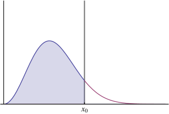
Figure 5: Probability density function for the theoretical variable $x$. The shaded are is the probability Eq. (68).

If $P_{\leq}$ is found to be too small or, equivalently, too high, we might be tempted to interpret $x_{0}$ as “anomalous” according to this model. However, this definition of probability assumes that $x_{0}$ was measured with infinite precision, and so it says nothing about an important question we must deal with: typically, the measurement of $x_{0}$ has an uncertainty which needs to be folded into the final probabilities that the observations match the theoretical expectations.

Moreover, since no two equally prepared experiments will ever return the same value $x_{0}$, our measurements should also be regarded as random events. In a more rigorous approach, we would have to consider $x_{0}$ itself as one realization of a random variable, conditioned to the distribution of the signal. In the case of CMB, however, this would be only part of the whole picture, since the randomness of the measurements of $x_{0}$ should also be related to the way this data is reduced to its final form. This happens because different map cleaning procedures will lead to slightly different values for $x_{0}$. This difference induces a variance in the data which reflects the remaining foreground contamination of the temperature map. We will elaborate more on this point through a concrete example, after we show how Eq. (68) may be changed in order to include the indeterminacy of cosmological measurements.

6.2 Convolving probabilities

The question we want to answer is: how to calculate the probability of $x$ being smaller than our measurements when the latter are also random events? Let us suppose that our measurement is described by the random variable $y$ and that $x_{0}$ is its most probable value. The probability of having $x\leq y$ is simply the probability of having

$$z\equiv x-y\leq 0$$

for some particular realization of the variable $y$. It should be clear by now that if we know the pdf of $z$, the probability we are looking for is simply the area under this distribution for $-\infty\leq z\leq 0$. The probability $P_{\leq}$ of $z$ being smaller or equal to zero can be calculated as:

$$P_{\leq}\equiv P\{(x,y)|x-y\leq 0\}=\iintop_{x-y\,\leq 0}\mathcal{P}(x,y)\,dx\,dy\,.$$

Now, under the hypothesis of independence of $x$ and $y$ we have $\mathcal{P}(x,y)=\mathcal{P}_{\scriptsize{\mbox{th}}}(x)\mathcal{P}_{\scriptsize{\mbox{obs}}}(y)$, where $\mathcal{P}_{\scriptsize{\mbox{obs}}}$ is the (normalized) probability distribution function of the variable $y$. We can therefore rewrite the last expression as

$$P_{\leq}=\int_{-\infty}^{\infty}\left[\int_{-\infty}^{y}\mathcal{P}_{\scriptsize{\mbox{th}}}(x)\,dx\right]\mathcal{P}_{\scriptsize{\mbox{obs}}}(y)\,dy\,.$$

If we now hold $y$ fixed and do the change of variables $x=u+y$, we get

$$P_{\leq}=\int_{-\infty}^{0}\left[\int_{-\infty}^{\infty}\mathcal{P}_{\scriptsize{\mbox{th}}}(u+y)\mathcal{P}_{\scriptsize{\mbox{obs}}}(y)\,dy\right]\,du\,.$$

where we have changed the position of the integrals. The reader will now notice that term inside brackets is precisely the pdf we were looking for. Since there is nothing special about the variable $y$, we can equally well hold $x$ fixed and repeat the calculus, obtaining the symmetric version of this result. In fact, the final pdf for $z$ is nothing else than the convolution of the pdf’s of each variable [77]:

$$\mathcal{P}(z)\equiv\left(\mathcal{P}_{\scriptsize{\mbox{obs}}}*\mathcal{P}_{\scriptsize{\mbox{th}}}\right)(z) = \int_{-\infty}^{\infty}\mathcal{P}_{\scriptsize{\mbox{obs}}}(y)\mathcal{P}_{\scriptsize{\mbox{th}}}(z\pm y)\,dy\,$$ (69)

$$= \int_{-\infty}^{\infty}\mathcal{P}_{\scriptsize{\mbox{obs}}}(x\mp z)\mathcal{P}_{\scriptsize{\mbox{th}}}(x)\,dx\,.$$

where the plus (minus) sign refers to the difference (sum) of $x$ and $y$. Integrating this pdf from $(-\infty,0]$ we get our answer

$$P_{\leq}\equiv\int_{-\infty}^{0}\mathcal{P}(z)dz\,.$$ (70)

As a consistency check, notice that in the limit where observations are made with infinite precision, $\mathcal{P}_{\scriptsize{\mbox{obs}}}(y)$ becomes a delta function and we have:

$$P_{\leq}=\int_{-\infty}^{0}\int_{-\infty}^{+\infty}\delta(y-x_{0})\mathcal{P}_{\scriptsize{\mbox{th}}}(z\pm y)dydz=\int_{-\infty}^{\pm x_{0}}\mathcal{P}_{\scriptsize{\mbox{th}}}(x)dx$$

which agrees with our previous definition. The reader must be careful, though, not to think of Eq. (68) as some lower bound to Eq. (70). Since none of the pdf’s appearing in Eq. (69) are necessarily symmetric, a large distance from $x_{0}$ to the most probable (not the mean!) value $x$ would not, by itself, constitute sufficient grounds to claim that the measured value of this observable is “unusual” in any sense, simply because a large overlap between the two pdf’s can render the result usual according to Eq. (70).

To illustrate this point, let us calculate $P_{\leq}$ using Eq. (68) and Eq. (70) for the pdf’s which appear in Fig. 6. For pedagogical reasons, we have chosen $\mathcal{P}_{\scriptsize{\mbox{th}}}$ and $\mathcal{P}_{\scriptsize{\mbox{obs}}}$ as positively (Maxwell distribution) and negatively (Gumbel distribution) skewed pdf’s, respectively. The convolved distribution appears as the solid (black) line. For these pdf’s, Eq. (68) gives $99.2\%$, while Eq. (70) gives $93.6\%$ of chance of $x$ being smaller than the observed $x_{0}$; all pdf’s were normalized to one.

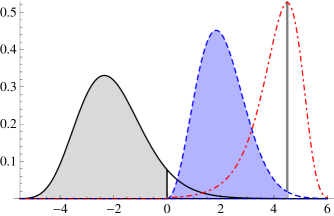
Figure 6: Probability density functions for $x$ (blue, dashed line), $y$ (red, dot-dashed line) and $z$ (solid line.) The shaded area gives the probability of $x$ being smaller than $x_{0}$ (dashed vertical line.) See the text for more details.

7 A $\chi^{2}$ test of statistical isotropy

Although the last example was constructed to emphasize an important feature of the formalism developed in §6, cosmological observables designed to measure deviations of either gaussianity or statistical isotropy will often follow asymmetric distributions. The intrinsic uncertainties of cosmological measurements, specially the ones originating from map cleaning procedures, may be crucial when searching for any map’s anomalies. We will now make a concrete application of this formalism using the angular-planar chi-square test developed in §5.1

7.1 $\Lambda$CDM model

In the simplest realization of the $\Lambda$CDM model, the covariance matrix of temperature maps is determined by $\langle a_{\ell_{1}m_{1}}a_{\ell_{2}m_{2}}\rangle=(-1)^{m_{2}}C_{\ell_{1}}\delta_{\ell_{1}\ell_{2}}\delta_{m_{1},-m_{2}}$. Using this expression in (64), we find that

$$\mathcal{C}_{\ell}^{lm}\;\overset{\textrm{(SI)}}{=}\;C_{\ell}\delta_{l0}\delta_{m0}\,.$$ (71)

On the other hand, if the only non-zero $\mathcal{C}_{\ell}^{lm}$’s are given by $l=m=0$, then $\mathcal{C}_{\ell}^{00}=C_{\ell}$. Therefore, statistical isotropy is achieved if and only if the angular-planar power spectrum is of the form (71). Since we are only interested in nontrivial planar modulations, we will restrict our analysis to the cases where $l\neq 0$, that is

$$\mathcal{C}_{\ell}^{lm}=0\,,\quad(l\geq 2)\,$$ (72)

where, we remind the reader, the parity of $\ell$ comes from the symmetry (24).

For this particular model, we can also calculate the covariance matrix of the estimator (66) explicitly. Using the null hypothesis above, we find after some algebra that

$$\langle(\widehat{\mathcal{C}}_{\ell}^{\;lm})^{*}\widehat{\mathcal{C}}_{\ell}^{\;l^{\prime}m^{\prime}}\rangle=8\pi^{2}\sum_{\ell_{1},\ell_{2}}C_{\ell_{1}}C_{\ell_{2}}\left(I_{\ell_{1}\ell_{2}}^{l,\ell}\right)^{2}\delta_{ll^{\prime}}\delta_{mm^{\prime}}\,.$$ (73)

This matrix has some interesting properties. First, note that the planar degrees of freedom are independent in this case (which justifies the $(2l+1)^{-1}$) factor introduced in Eq. (67).) Second, its diagonal elements are given by the variance $(\sigma^{lm}_{\ell})^{2}=\langle(\widehat{\mathcal{C}}^{\;lm}_{\ell})^{*}\widehat{\mathcal{C}}^{\;lm}_{\ell}\rangle$, which now becomes $m$-independent:

$$\left(\sigma^{lm}_{\ell}\right)^{2}\;\rightarrow\left(\sigma^{l}_{\ell}\right)^{2}=8\pi^{2}\sum_{\ell_{1},\ell_{2}}C_{\ell_{1}}C_{\ell_{2}}\left(I_{\ell_{1}\ell_{2}}^{l,\ell}\right)^{2}\,.$$ (74)

Therefore, for the particular case of the $\Lambda$CDM model, the chi-square test (67) gets even simpler. Using (72) and (74), we find

$$(\chi^{2}_{\nu})^{l}_{\ell}=\frac{1}{2l+1}\sum_{m=-l}^{l}\frac{|\widehat{\mathcal{C}}^{\;lm}_{\ell}|^{2}}{(\sigma^{l}_{\ell})^{2}}\,.$$ (75)

It is now clear that if the data under analysis are really described by this model, then it must be true that

$$\langle(\chi^{2}_{\nu})^{l}_{\ell}\rangle=\frac{1}{2l+1}\sum_{m=-l}^{l}\frac{\langle(\widehat{\mathcal{C}}^{\;lm}_{\ell})^{*}\widehat{\mathcal{C}}^{\;lm}_{\ell}\rangle}{(\sigma^{l}_{\ell})^{2}}=1\,$$

where we have used (74). This shows that any large deviation of this test from unity will be an indication of planar modulation in temperature maps, up, of course, to error bars. For convenience, let us define a new quantity as

$$\overline{\chi}^{\,l}_{\ell}\equiv(\chi^{2}_{\nu})^{l}_{\ell}-1\,$$ (76)

which will quantify anisotropies whenever $\overline{\chi}^{\,l}_{\ell}$ is significantly positive or negative.

This generalized chi-square test furnishes a complete prescription when searching for planar modulations of temperature in CMB maps. We emphasize, though, that for a given CMB map, the chi-square analysis must be done entirely in terms of that map’s data. Since we are performing a model-independent test, we are not allowed to introduce fiducial biases in the analysis (for example, by calculating $\sigma^{l}_{\ell}$ using $C_{\ell}^{\scriptsize{\rm{model}}}$), which would only include our a priori prejudices about what the map’s anisotropies should look like. Since the $C_{\ell}$’s are, by construction, a measure of statistical isotropy. Consequently, an “anomalous” detection of $C_{\ell}$’s is by no means a measure of statistical anisotropy, and it is this particular value that should be used in (76) if we want to find deviations of isotropy, regardless of how high/low it is.

7.2 Searching for planar signatures in WMAP

In order to apply the test (76) to the 5-year WMAP data [14, 11], we will define two new variables

$$x\equiv(\bar{\chi}^{2})_{\ell(\scriptsize{\mbox{th}})}^{l}\,,\quad y\equiv(\bar{\chi}^{2})_{\ell(\scriptsize{\mbox{obs}})}^{l}\,,\quad$$

which will be jointly analyzed using the formalism of section §6. Still, there remains the question of how to obtain their pdf’s. These functions can be obtained numerically provided that the number of realizations of each variable is large enough, since in this case their histograms can be considered as piecewise constant functions which approximate the real pdf’s. For the case of the (theoretical) variable $x$ defined above we have run $2\times 10^{4}$ Monte Carlo simulations of Gaussian and statistically isotropic CMB maps using the $\Lambda\mbox{CDM}$ best-fit $C_{\ell}$’s provided by the WMAP team [78]. With these maps we have then constructed $2\times 10^{4}$ realizations of the variable $x$.

The simulation of the (observational) variable $y$ is more difficult, and depends on the way we estimate contamination from residual foregrounds in CMB maps. As is well-known, not only instrumental noise, but systematic errors (e.g., in the map-making process), the inhomogeneous scanning of the sky (i.e., the exposure function of the probe), or unremoved foreground emissions (even after applying a cut-sky mask) could corrupt – at distinct levels – the CMB data.

Foreground contamination, on the other hand, may have several different sources, many of which are far beyond our present scopes. However, since different teams apply distinct procedures on the raw data in order to produce a final map, we will make the hypothesis that maps cleaned by different teams represent – to a good extent – “independent” CMB maps. Therefore, we can estimate the residual foreground contaminations by comparing these different foreground-cleaned maps.

Full sky maps	References
Hinshaw et. al.	[14, 79]
de Oliveira-Costa et. al.	[80]
Kim et. al.	[81]
Park et. al.	[82]
Delabrouille et. al.	[83]

Table 1: Full-sky foreground cleaned CMB maps from WMAP data used in our analysis to estimate the variable $y$ (see the text for more details.) Note that the reference [81] includes the analysis of maps from the three and five years WMAP releases.

In fact, the WMAP science team has made substantial efforts to improve the data products by minimizing the contaminating effects caused by diffuse galactic foregrounds, astrophysical point-sources, artifacts from the instruments and measurement process, and systematic errors [84, 85]. As a result, multi-frequency foreground-cleaned full-sky CMB maps were produced, named Internal Linear Combination maps, corresponding to three and five year WMAP data [14, 79]. To account for the mentioned randomness, systematic, and contaminating effects of the CMB data, we will use in our analyses several full-sky foreground-cleaned CMB maps, listed in Table 1, which were produced using both the three and five year WMAP data.

The prescription we adopt to determine the distribution of the observational variable $y$ is as follows: we simulate Gaussian random $a_{\ell m}$’s in such a way that their central values are given by the five year ILC5 data [79, 14], and with a variance which is estimated from the sample standard deviation of all the maps listed in Table 1. So, for example, suppose we have $n$ different full-sky temperature maps at hand and we want to estimate the randomness inherent in the determination of, let’s say, $a_{32}$. Therefore, we take

$$\mathcal{N}(a_{32}^{\scriptsize{\mbox{ILC5}}},\sigma_{32})\;\rightarrow\;a_{32}\,,$$ (77)

with

$$\sigma_{32}=\sqrt{\frac{1}{n-1}\sum_{i=1}^{n}(a_{32}^{i}-\bar{a}_{32})^{2}}\qquad\mbox{and}\qquad\bar{a}_{32}=\frac{1}{n}\sum_{i=1}^{n}a_{32}^{i}\,,$$ (78)

where $\mathcal{N}(\mu,\sigma)$ represents a Gaussian distribution with mean $\mu$ and standard deviation $\sigma$. Note that if the residual contamination is indeed weak, then the sample variance above will be small, and our procedure will reduce to the standard way of calculating probabilities. As for the use of a Gaussian in (77), this choice was dictated not only by simplicity, but rather by the fact that the propagation of uncertainties in physical experiments are usually assumed to follow a normal distribution. Note however that there are some instrumental uncertainties, such as beam or gain uncertainties, which will not in general follow normal distributions. In fact, some of them may even fail to be additive, meaning that our convolution formula will be inapplicable in these cases. In our analysis, we have focused only on foreground residuals, where the normality hypothesis is reasonable.

7.3 Full-sky maps

Following this procedure, we have used the full-sky maps shown in Table (1) to construct $10^{4}$ Gaussian random $a_{\ell m}$’s, which were then used to calculate $10^{4}$ realizations of $y=(\bar{\chi}^{2})^{l}_{\ell({\rm obs})}$. With those variables we constructed histograms which, together with the histograms for the (full-sky) variable $x$, were used to calculate the final probability (70). We have restricted our analysis to the range of values $(\ell,l)\in[2,10]$, since the low multipolar sector (i.e., large angular scales) is where most of the anomalies were reported. The resulting histograms and pdf’s are shown in Fig. 7, and the final probabilities we obtained are show in Table 2.

$l\backslash\ell$	2	3	4	5	6	7	8	9	10
2	81.1%	73.7%	54.1%	6.1%	80.7%	46.4%	36.9%	47.5%	81.8%
4	74.0%	72.6%	55.0%	39.6%	74.2%	93.2%	51.6%	55.4%	56.3%
6	78.1%	80.7%	69.3%	52.3%	33.6%	80.0%	95.0%	50.3%	82.2%
8	63.5%	87.7%	18.8%	51.5%	21.4%	66.4%	31.6%	27.5%	82.3%
10	67.9%	50.0%	61.0%	8.7%	37.7%	59.5%	36.6%	29.2%	35.7%

Table 3: Final probabilities of obtaining, in a random $\Lambda$CDM Universe, a chi-square value smaller or equal to $(\bar{\chi}^{2})_{\ell(\scriptsize{\rm obs})}^{l}$, as given by full-sky temperature maps.

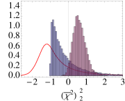
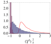
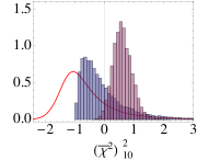
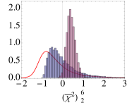
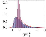
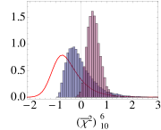
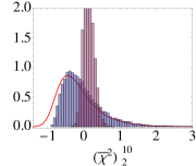
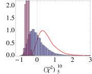
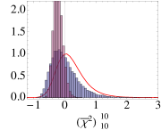
Figure 7: Histograms for $(\bar{\chi}^{2})_{\ell(\scriptsize{\mbox{th}})}^{l}$ (blue), $(\bar{\chi}^{2})_{\ell(\scriptsize{\mbox{obs}})}^{l}$ (purple) and for the difference $(\bar{\chi}^{2})_{\ell(\scriptsize{\mbox{th}})}^{l}-(\bar{\chi}^{2})_{\ell(\scriptsize{\mbox{obs}})}^{l}$ (solid, red line). We show only a few representative figures. The final probabilities are shown in Table 2 and correspond to the area under the solid curve from $-\infty$ to $0$. All pdf’s are normalized to 1.

Overall, our results show no significant planar deviations of anisotropy in WMAP data. The most unlikely individual values in Table (2) are in the sectors $(l,\ell)$ given by $(2,5)$, $(10,5)$, $(4,7)$ and $(6,8)$, and are all above a relative chance of 5% of either being too negative [$\left(2,5\right)$, $\left(10,5\right)$] or too positive [$(4,7)$, $(6,8)$]. However, it is perhaps worth mentioning that not only the individual values of $(\bar{\chi}^{2})^{l}_{\ell}$ are relevant, their coherence over a range of angular or planar momenta also carries interesting information. So, for example, a set of $(\bar{\chi}^{2})^{l}_{\ell}$’s which are all individually within the cosmic variance bounds, but which are all positive (or negative) can be an indication of an excess (or lack) of planar modulation. This type of coherent behavior appears in the following cases: $(\bar{\chi}^{2})^{l}_{2}$, $(\bar{\chi}^{2})^{l}_{3}$ and, to a lesser extent, $(\bar{\chi}^{2})^{4}_{\ell}$ – see Table 2. The angular quadrupole $\ell=2$, as well as the angular octupole $\ell=3$, have all positive planar spectra (for all values of $l$ which we were able to compute), indicated by probabilities larger than 50%. The planar hexadecupole $l=4$ also has 8 out of 9 angular spectra assuming positive values (only $\ell=5$ is negative).

The data analyzed in this Section relates to the full-sky maps, which are certainly still affected by residual galactic foregrounds. The reader interested in the complete analysis, including data from masked CMB maps, can check reference [28].

8 Conclusions

We know our Universe is not perfectly Gaussian, or homogeneous, or isotropic. The deviations from an idealized picture (or the lack thereof), whether predictably small or surprisingly large, can tell us a great deal about the Universe we live in. Since the types of physical mechanisms behind deviations from perfect gaussianity, homogeneity or isotropy are typically very different, we should try to measure these individual features separately – whenever possible or practical.

Recently it has been suggested that some of the most discussed anomalies in the CMB can be explained away [86], or that the evidence for them is statistically weak [87]. But even if it turns out that our Universe is a plain vanilla kind of place, where everything goes according to the inflationary theorist’s dreams, we would still need to analyze it with tools that allow us to check the standard picture against the data. In addition, local physics (related to the solar system, or our galaxy), as well as instrumental quirks, tend to leave imprints on the CMB which are clearly anisotropic, but have a certain coherence which can be detected, and possibly corrected for, with the help of these checks.

However, in an era where at least the large-scale maps of the CMB are likely to remain basically unchanged, we should be careful not to over analize the data with the benefit of an ever greater hindsight (put another way, a posteriori conundrums only get worse with time.) This can only be achieved if we find natural and generally agreed-upon classifications of the types of deviations that may occur, without too much guidance from what the data is telling us. We believe that focusing on the possible underlying symmetries, with perhaps some guidance from group-theoretic arguments, is one way to settle these issues. We have presented a few methods along these lines, one using multipole vectors, the other using a natural generalization of the two-point correlation function – and other methods have been presented in this Review.

Perhaps the best indication that we are on the right track is the fact that most of these methods are applicable in other areas of physics and astronomy – and that in some cases we have adapted tests of anisotropy from other areas, such as scattering theory and the theory of angular momentum in quantum mechanics. So, even if these anomalies eventually perish, they will be survived by the powerful methods that have been devised to test them.

Acknowledgements

We would like to thank Glenn Starkman and Yuri Shtanov for enlightening discussions during the development of this work. This work was supported by FAPESP and CNPq.

Appendix A Geometrical identities and derivations

Wigner $D$-functions

From the unitarity of the rotation operators $D(R)$, we have

$$\sum_{m}D_{m^{\prime}m}^{\ell}(\omega_{1})D_{m^{\prime\prime}m}^{\ell}(\omega_{2})=D_{m^{\prime}m^{\prime\prime}}^{\ell}(\omega_{1}\omega_{2})\,.$$

If $\omega_{2}=\omega_{1}^{-1}$, then using the identity $D_{m^{\prime\prime}m}^{\ell}(\omega^{-1})=D_{m^{\prime\prime}m}^{*\ell}(\omega)$, we find

$$\sum_{m}D_{m^{\prime}m}^{\ell}(\omega_{1})D_{m^{\prime\prime}m}^{*\ell}(\omega_{1})=\delta_{m^{\prime}m^{\prime\prime}}\,.$$

Gaunt integral

The definition of the Gaunt integral used in this paper is

$$\mathcal{G}_{m_{1}m_{2}m_{3}}^{\ell_{1}\ell_{2}\ell_{3}}=(-1)^{m_{1}}\int d^{2}{\hat{n}}\;Y_{\ell_{1},-m_{1}}(\hat{n})Y_{\ell_{2}m_{2}}(\hat{n})Y_{\ell_{2}m_{2}}(\hat{n})\,.$$

3-j symbols

We present here some useful identities related to the 3-j symbols:

• Isotropic limit

  $$\left(\begin{array}[]{ccc}l_{1}&l_{2}&0\\ m_{1}&m_{2}&0\end{array}\right)=\frac{(-1)^{l_{2}-m_{1}}}{\sqrt{2l_{1}+1}}\delta_{l_{1}l_{2}}\delta_{m_{1},-m_{2}}\,.$$

• Parity and permutations

  $$\left(\begin{array}[]{ccc}l_{1}&l_{2}&l\\ m_{1}&m_{2}&m\end{array}\right) = \left(\begin{array}[]{ccc}l&l_{1}&l_{2}\\ m&m_{1}&m_{2}\end{array}\right)$$

  $$= (-1)^{l_{1}+l_{2}+l}\left(\begin{array}[]{ccc}l_{2}&l_{1}&l\\ m_{2}&m_{1}&m\end{array}\right)$$

  $$= (-1)^{l_{1}+l_{2}+l}\left(\begin{array}[]{ccc}l_{1}&l_{2}&l\\ -m_{1}&-m_{2}&-m\end{array}\right)\,.$$

• Orthogonality

  $$\sum_{m_{1}=-l_{1}}^{l_{1}}\sum_{m_{2}=-l_{2}}^{l_{2}}\left(\begin{array}[]{ ccc}l_{1}&l_{2}&l_{3}\\ m_{1}&m_{2}&m_{3}\end{array}\right)\left(\begin{array}[]{ccc}l_{1}&l_{2}&l_{3}^{\prime}\\ m_{1}&m_{2}&m_{3}^{\prime}\end{array}\right) = \frac{\delta_{l_{3}l_{3}^{\prime}}\delta_{m_{3}m_{3}^{\prime}}}{2l_{3}+1}$$

  $$\sum_{l_{1}=|l_{2}-l_{3}|}^{l_{2}+l_{3}}\sum_{m_{1}=-l_{1}}^{l_{1}}(2l+1)\left(\begin{array}[]{ccc}l_{1}&l_{2}&l_{3}\\ m_{1}&m_{2}&m_{3}\end{array}\right)\left(\begin{array}[]{ccc}l_{1}&l_{2}&l_{4}\\ m_{1}&m_{2}^{\prime}&m_{3}^{\prime}\end{array}\right) = \delta_{m_{2}m_{2}^{\prime}}\delta_{m_{3}m_{3}^{\prime}}$$

  $$\sum_{m=-l}^{l}(-1)^{l-m}\left(\begin{array}[]{ccc}l&l&\ell\\ m&-m&0\end{array}\right) = \sqrt{2l+1}\delta_{\ell,0}\,.$$

  The last expression is particularly useful in the derivation of (71).

Derivation of (64)

We start by equating expressions (62) and (20)

$$\sum_{\ell}\sum_{l,m}\frac{2\ell+1}{\sqrt{4\pi}}\,\mathcal{C}_{\ell}^{lm}\,P_{\ell}(\cos\vartheta)Y_{lm}(\hat{n})=\sum_{\ell_{1},m_{1}}\sum_{\ell_{2},m_{2}}\langle a_{\ell_{1}m_{1}}a_{\ell_{2}m_{2}}^{*}\rangle Y_{\ell_{1}m_{1}}(\hat{n}_{1})Y_{\ell_{2}m_{2}}(\hat{n}_{2})\,.$$ (85)

As mentioned in the main text, the inversion of $\mathcal{C}_{\ell}^{lm}$ as a function of the $a_{\ell m}$’s is not a trivial task, since the angles $(\Theta,\Phi,\theta)$ depend non-linearly on the angles $(\theta_{1},\varphi_{1},\theta_{2},\varphi_{2})$. The easiest way to achieve this goal is to pick up a coordinate system where only the $\theta$ dependence is present. After integrating it out, we rotate our coordinate system using three Euler angles to recover back the $(\Theta,\Phi)$ dependence, which can then be integrated with the help of some Wigner matrices identities. We start by positioning the vectors $\hat{n}_{1}$ and $\hat{n}_{2}$ in the $xy$ plane, i.e, we chose $\hat{n}_{1}=(\pi/2,\phi_{1})$, $\hat{n}_{2}=(\pi/2,\phi_{2})$. By (63) we then have $\cos\vartheta=\cos(\phi_{1}-\phi_{2})$. Using the relation [41]

$$Y_{\ell m}(\pi/2,\phi)=\lambda_{\ell m}e^{im\phi},\quad\lambda_{\ell m}=\begin{cases}(-1)^{\frac{\ell+m}{2}}\sqrt{\frac{2\ell+1}{4\pi}\frac{(\ell+m-1)!!}{(\ell+m)!!}\frac{(\ell-m-1)!!}{(\ell-m)!!}}\quad&\mbox{if}\quad\ell+m\in 2\mathbb{N}\\ 0&\mbox{otherwise}\end{cases}$$ (86)

we can integrate the $\theta$ dependence on both sides of (85). This gives us

$$\frac{1}{\sqrt{\pi}}\sum_{l,m}\mathcal{C}_{\ell}^{lm}Y_{lm}(0,0)=\sum_{\ell_{1},m_{1}}\sum_{\ell_{2},m_{2}}\langle a_{\ell_{1}m_{1}}a_{\ell_{2}m_{2}}^{*}\rangle I_{\ell_{1}m_{1}\ell_{2}m_{2}}^{\ell}$$ (87)

where we have introduced the following definition

$$I_{\ell_{1}m_{1}\ell_{2}m_{2}}^{\ell}\equiv-\lambda_{\ell_{1}m_{1}}\lambda_{\ell_{2}m_{2}}\int_{0}^{\pi}P_{\ell}(\cos(\varphi_{1}-\varphi_{2}))e^{i(m_{1}\varphi_{1}-m_{2}\varphi_{2})}d(\cos(\varphi_{1}-\varphi_{2}))\,.$$ (88)

We need now to integrate out the $\Theta$ and $\Phi$ dependence in the right-hand side of (87) which was hidden due to our choice of a particular coordinate system. In order to do that, we keep the vectors $\hat{n}_{1}$ and $\hat{n}_{2}$ fixed and make a rotation of our coordinate system using three Euler angles $\omega=\{\alpha,\beta,\gamma\}$. This rotation changes the coefficients $\mathcal{C}_{\ell}^{lm}$’s and $a_{\ell m}$’s according to

$$a_{\ell m}=\sum_{m^{\prime}}D_{mm^{\prime}}^{\ell}(\omega)\widetilde{a}_{\ell m^{\prime}}\,,\qquad\mathcal{C}_{\ell}^{lm}=\sum_{m^{\prime}}D_{mm^{\prime}}^{l}(\omega)\widetilde{\mathcal{C}}_{\ell}^{lm^{\prime}}$$

where $\widetilde{\mathcal{C}}_{\ell}^{lm}$ and $\widetilde{a}_{lm}$ are the multipolar coefficients in the new coordinate system and where $D_{mm^{\prime}}^{l}(\omega)$ are the elements of the Wigner rotation matrix. The advantage of positioning the vectors $\hat{n}_{1}$ and $\hat{n}_{2}$ in the plane $xy$ is that now the angles $\Theta$ and $\Phi$ are given precisely by the Euler angles $\beta$ and $\gamma$, regardless of the value of $\alpha$

$$\sum_{l,m}\mathcal{C}_{\ell}^{lm}Y_{lm}(0,0)=\sum_{l,m^{\prime}}\widetilde{\mathcal{C}}_{\ell}^{lm^{\prime}}\left(\sum_{m}D_{mm^{\prime}}^{l}(\alpha,\beta,\gamma)Y_{lm}(0,0)\right)=\sum_{l,m^{\prime}}\widetilde{\mathcal{C}}_{\ell}^{lm^{\prime}}Y_{l,-m}(\beta,\gamma)$$

where in the last step we have used $Y_{lm}(0,0)=\sqrt{(2l+1)/4\pi}\,\delta_{m0}$. Therefore, in our new coordinate system we have (dropping the “ $\widetilde{}$ ” in our notation)

$$\frac{1}{2\pi}\sum_{l,m}\mathcal{C}_{\ell}^{lm}D_{0m}^{l}(\omega)\sqrt{2l+1}=\sum_{\ell_{1},m_{1}}\sum_{\ell_{2},m_{2}}\langle a_{\ell_{1}m_{1}}a_{\ell_{2}m_{2}}^{*}\rangle\sum_{m_{1}^{\prime}m_{2}^{\prime}}I_{\ell_{1}m_{1}^{\prime}\ell_{2}m_{2}^{\prime}}^{\ell}D_{m_{1}^{\prime}m_{1}}^{\ell_{1}}(\omega)D_{m_{2}^{\prime}m_{2}}^{\ell_{2}*}(\omega)\,.$$

We may now isolate $\mathcal{C}_{\ell}^{lm}$ using the identities [41]

$$\int d\omega\,D_{m_{1}m_{1}^{\prime}}^{l_{1}*}(\omega)D_{m_{2}m_{2}^{\prime}}^{l_{2}}(\omega) = \frac{8\pi^{2}}{2l_{1}+1}\delta_{l_{1}l_{2}}\delta_{m_{1}m_{2}}\delta_{m_{1}^{\prime}m_{2}^{\prime}}$$

$$\int d\omega\,D_{m_{1}^{\prime}m_{1}}^{l_{1}}(\omega)D_{m_{2}^{\prime}m_{2}}^{l_{2}}(\omega)D_{m_{3}^{\prime}m_{3}}^{l_{3}}(\omega) = 8\pi^{2}\left(\begin{array}[]{ccc}l_{1}&l_{2}&l_{3}\\ m_{1}^{\prime}&m_{2}^{\prime}&m_{3}^{\prime}\end{array}\right)\left(\begin{array}[]{ccc}l_{1}&l_{2}&l_{3}\\ m_{1}&m_{2}&m_{3}\end{array}\right)$$

where $d\omega=\sin\beta d\beta d\alpha d\gamma$, to obtain

$$\frac{1}{\sqrt{2l+1}}\mathcal{C}_{\ell}^{lm} = 2\pi\sum_{\ell_{1},m_{1}}\sum_{\ell_{2},m_{2}}\langle a_{\ell_{1}m_{1}}a_{\ell_{2}m_{2}}^{*}\rangle\sum_{m_{1}^{\prime}m_{2}^{\prime}}I_{\ell_{1}m_{1}^{\prime}\ell_{2}m_{2}^{\prime}}^{\ell}(-1)^{m_{2}+m_{2}^{\prime}+m}$$

$$\qquad\qquad\qquad\qquad\left(\begin{array}[]{ccc}\ell_{1}&\ell_{2}&l\\ m_{1}^{\prime}&-m_{2}^{\prime}&0\end{array}\right)\!\left(\begin{array}[]{ccc}\ell_{1}&\ell_{2}&l\\ m_{1}&-m_{2}&-m\end{array}\right)\,.$$

If we now redefine $-m_{2}\rightarrow m_{2}$ and note that the first 3-j symbol above is identically zero unless $m^{\prime}_{1}=m^{\prime}_{2}$, we finally obtain (64).

Some properties of the integral (65)

The geometrical coefficients $I_{\ell_{1}\ell_{2}}^{l,\ell}$ defined in (65) has many interesting properties which can be explored in order to speed up numerical computation of (64). First, we note that it is symmetric under permutation of $\ell_{1}$ and $\ell_{2}$:

$$I_{\ell_{1}\ell_{2}}^{l,\ell} = \sum_{m}I_{\ell_{1}m\ell_{2}m}^{\ell}(-1)^{m}\left(\begin{array}[]{ccc}\ell_{1}&\ell_{2}&l\\ m&-m&0\end{array}\right)$$

$$= \sum_{m}I_{\ell_{2}m\ell_{1}m}^{\ell}(-1)^{m+\ell_{1}+\ell_{2}+l}\left(\begin{array}[]{ccc}\ell_{2}&\ell_{1}&l\\ -m&m&0\end{array}\right)$$

$$= \sum_{m}I_{\ell_{2}m\ell_{1}m}^{\ell}(-1)^{m+2(\ell_{1}+\ell_{2}+l)}\left(\begin{array}[]{ccc}\ell_{2}&\ell_{1}&l\\ m&-m&0\end{array}\right)$$

$$= I_{\ell_{2}\ell_{1}}^{l,\ell}\,.$$

Some of the other properties are a consequence of the integral $I_{\ell_{1}m\ell_{2}m}^{\ell}$ defined in (88). We may note for example that, due to the symmetry of the $\lambda_{\ell m}$ coefficient defined in (86), we will have:

Furthermore, the $\lambda_{\ell m}$ coefficients restrict the $m$ summation above to their values which obey: $m+\ell_{1}+\ell_{2}=\mbox{even}$. If we further notice that (88) is proportional to the integral of a integral of the form $\int_{-1}^{1}P_{\ell}(\cos\theta)\cos m\theta\,d\theta$, and that this integral is zero unless $\ell+m=\mbox{even}$, we conclude that

Besides, using the fact that the integral $\int_{-1}^{1}P_{\ell}(\cos\theta)\cos m\theta\,d\theta$ is zero for any $m<\ell$, we find

We finally comment on the special case where $l=0$, for which we have

However

$$\sum_{m=-\ell^{\prime}}^{\ell^{\prime}}I_{\ell^{\prime}m\ell^{\prime}m}^{\ell} = \int_{0}^{\pi}P_{\ell}(\cos\vartheta)\left(\sum_{m=-\ell^{\prime}}^{\ell^{\prime}}\frac{(2\ell^{\prime}+1)}{4\pi}\frac{(\ell^{\prime}+m-1)!!}{(\ell^{\prime}+m)!!}\frac{(\ell^{\prime}-m-1)!!}{(\ell^{\prime}-m)!!}e^{im\vartheta}\right)d(-\cos\vartheta)$$

$$= \frac{2\ell^{\prime}+1}{4\pi}\int_{-1}^{1}P_{\ell}(x)P_{\ell^{\prime}}(x)dx$$

$$= \frac{1}{2\pi}\delta_{\ell\ell^{\prime}}\,.$$

where in the derivation above we have made use of the Fourier series expansion of the Legendre polynomial. So we conclude that

which is needed in the derivation of (71).

References

- [1] V. Mukhanov, Physical Foundations of Cosmology (Cambridge University Press, 2005).
- [2] S. Weinberg, Cosmology (Oxford Univ. Press, 2008).
- [3] P. Peter and J.-P. Uzan, Primordial Cosmology (Oxford Univ. Press, 2009).
- [4] W. Hu, U. Seljak, M. J. White, and M. Zaldarriaga, Phys. Rev. D57, 3290 (1998), astro-ph/9709066.
- [5] W. Hu, Ann. Phys. 303, 203 (2003), astro-ph/0210696.
- [6] S. Dodelson, Modern Cosmology (Academic Press, 2003).
- [7] J. M. Maldacena, JHEP 05, 013 (2003), astro-ph/0210603.
- [8] S. Weinberg, Phys. Rev. D72, 043514 (2005), hep-th/0506236.
- [9] S. Weinberg, Phys. Rev. D74, 023508 (2006), hep-th/0605244.
- [10] K. M. Huffenberger and U. Seljak, New Astron. 10, 491 (2005), astro-ph/0408066.
- [11] WMAP, E. Komatsu et al., Astrophys. J. Suppl. 180, 330 (2009), 0803.0547.
- [12] A. Bernui and M. J. Reboucas, Phys. Rev. D79, 063528 (2009), 0806.3758.
- [13] V. F. Mukhanov, H. A. Feldman, and R. H. Brandenberger, Phys. Rept. 215, 203 (1992).
- [14] WMAP, G. Hinshaw et al., Astrophys. J. Suppl. 180, 225 (2009), 0803.0732.
- [15] SDSS, M. Tegmark et al., Astrophys. J. 606, 702 (2004), astro-ph/0310725.
- [16] The 2dFGRS, S. Cole et al., Mon. Not. Roy. Astron. Soc. 362, 505 (2005), astro-ph/0501174.
- [17] Supernova Cosmology Project, S. Perlmutter et al., Astrophys. J. 517, 565 (1999), astro-ph/9812133.
- [18] Supernova Search Team, A. G. Riess et al., Astron. J. 116, 1009 (1998), astro-ph/9805201.
- [19] ESSENCE, W. M. Wood-Vasey et al., Astrophys. J. 666, 694 (2007), astro-ph/0701041.
- [20] WMAP, C. L. Bennett et al., Astrophys. J. Suppl. 148, 1 (2003), astro-ph/0302207.
- [21] G. F. Smoot et al., Astrophys. J. 396, L1 (1992).
- [22] A. de Oliveira-Costa, M. Tegmark, M. Zaldarriaga, and A. Hamilton, Phys. Rev. D69, 063516 (2004), astro-ph/0307282.
- [23] C. J. Copi, D. Huterer, and G. D. Starkman, Phys. Rev. D70, 043515 (2004), astro-ph/0310511.
- [24] D. J. Schwarz, G. D. Starkman, D. Huterer, and C. J. Copi, Phys. Rev. Lett. 93, 221301 (2004), astro-ph/0403353.
- [25] K. Land and J. Magueijo, Phys. Rev. Lett. 95, 071301 (2005), astro-ph/0502237.
- [26] C. J. Copi, D. Huterer, D. J. Schwarz, and G. D. Starkman, Mon. Not. Roy. Astron. Soc. 367, 79 (2006), astro-ph/0508047.
- [27] M. Tegmark, A. de Oliveira-Costa, and A. Hamilton, Phys. Rev. D68, 123523 (2003), astro-ph/0302496.
- [28] L. R. Abramo, A. Bernui, and T. S. Pereira, JCAP 0912, 013 (2009), 0909.5395.
- [29] A. Bernui, B. Mota, M. J. Reboucas, and R. Tavakol, Astron. Astrophys. 464, 479 (2007), astro-ph/0511666.
- [30] A. Bernui, Phys. Rev. D78, 063531 (2008), 0809.0934.
- [31] H. K. Eriksen, F. K. Hansen, A. J. Banday, K. M. Gorski, and P. B. Lilje, Astrophys. J. 605, 14 (2004), astro-ph/0307507.
- [32] H. K. Eriksen, A. J. Banday, K. M. Gorski, F. K. Hansen, and P. B. Lilje, Astrophys. J. 660, L81 (2007), astro-ph/0701089.
- [33] D. Pietrobon et al., (2009), arXiv:0905.3702.
- [34] L. R. Abramo, L. S. Jr., and C. A. Wuensche, Phys. Rev. D74, 083515 (2006), astro-ph/0605269.
- [35] L. R. Abramo, A. Bernui, I. S. Ferreira, T. Villela, and C. A. Wuensche, Phys. Rev. D74, 063506 (2006), astro-ph/0604346.
- [36] D. Hanson and A. Lewis, Phys. Rev. D80, 063004 (2009), 0908.0963.
- [37] A. R. Pullen and M. Kamionkowski, Phys. Rev. D76, 103529 (2007), 0709.1144.
- [38] T. S. Pereira, C. Pitrou, and J.-P. Uzan, JCAP 0709, 006 (2007), 0707.0736.
- [39] C. Pitrou, T. S. Pereira, and J.-P. Uzan, JCAP 0804, 004 (2008), 0801.3596.
- [40] A. E. Gumrukcuoglu, C. R. Contaldi, and M. Peloso, JCAP 0711, 005 (2007), 0707.4179.
- [41] D. A. Varshalovich, A. N. Moskalev, and V. K. Khersonsky, SINGAPORE, SINGAPORE: WORLD SCIENTIFIC (1988) 514p.
- [42] J.-P. Uzan, C. Clarkson, and G. F. R. Ellis, Phys. Rev. Lett. 100, 191303 (2008), 0801.0068.
- [43] S. Prunet, J.-P. Uzan, F. Bernardeau, and T. Brunier, Phys. Rev. D71, 083508 (2005), astro-ph/0406364.
- [44] P. G. Ferreira and J. Magueijo, Phys. Rev. D56, 4578 (1997), astro-ph/9704052.
- [45] J. N. Fry and A. L. Melott, NSF-ITP-84-143.
- [46] X. chun Luo, Astrophys. J. 427, L 71 (1994), astro-ph/9312004.
- [47] D. N. Spergel and D. M. Goldberg, Phys. Rev. D59, 103001 (1999), astro-ph/9811252.
- [48] W. Hu, Phys. Rev. D64, 083005 (2001), astro-ph/0105117.
- [49] E. Hivon et al., (2001), astro-ph/0105302.
- [50] L. Ackerman, S. M. Carroll, and M. B. Wise, Phys. Rev. D75, 083502 (2007), astro-ph/0701357.
- [51] Y. Shtanov and H. Pyatkovska, Phys. Rev. D80, 023521 (2009), 0904.1887.
- [52] J. P. Luminet, J. Weeks, A. Riazuelo, R. Lehoucq, and J. P. Uzan, Nature. 425, 593 (2003), astro-ph/0310253.
- [53] A. Riazuelo, J. Weeks, J.-P. Uzan, R. Lehoucq, and J.-P. Luminet, Phys. Rev. D69, 103518 (2004), astro-ph/0311314.
- [54] W. S. Hipolito-Ricaldi and G. I. Gomero, Phys. Rev. D72, 103008 (2005), astro-ph/0507238.
- [55] T. Kahniashvili, G. Lavrelashvili, and B. Ratra, Phys. Rev. D78, 063012 (2008), 0807.4239.
- [56] T. Kahniashvili, Y. Maravin, and A. Kosowsky, Phys. Rev. D80, 023009 (2009), 0806.1876.
- [57] A. Bernui and W. S. Hipolito-Ricaldi, Mon. Not. Roy. Astron. Soc. 389, 1453 (2008), 0807.1076.
- [58] C. Caprini, F. Finelli, D. Paoletti, and A. Riotto, JCAP 0906, 021 (2009), 0903.1420.
- [59] T. R. Seshadri and K. Subramanian, Phys. Rev. Lett. 103, 081303 (2009), 0902.4066.
- [60] C. Gordon, W. Hu, D. Huterer, and T. M. Crawford, Phys. Rev. D72, 103002 (2005), astro-ph/0509301.
- [61] L. Campanelli, P. Cea, and L. Tedesco, Phys. Rev. D76, 063007 (2007), 0706.3802.
- [62] L. Campanelli, (2009), arXiv:0907.3703.
- [63] A. L. Erickcek, M. Kamionkowski, and S. M. Carroll, Phys. Rev. D78, 123520 (2008), 0806.0377.
- [64] A. L. Erickcek, C. M. Hirata, and M. Kamionkowski, (2009), arXiv:0907.0705.
- [65] J. F. Donoghue, K. Dutta, and A. Ross, Phys. Rev. D80, 023526 (2009), astro-ph/0703455.
- [66] M. Kawasaki, K. Nakayama, T. Sekiguchi, T. Suyama, and F. Takahashi, JCAP 0811, 019 (2008), 0808.0009.
- [67] M. Kawasaki, K. Nakayama, T. Sekiguchi, T. Suyama, and F. Takahashi, JCAP 0901, 042 (2009), 0810.0208.
- [68] A. Hajian and T. Souradeep, Astrophys. J. 597, L5 (2003), astro-ph/0308001.
- [69] A. Hajian, T. Souradeep, and N. J. Cornish, Astrophys. J. 618, L63 (2004), astro-ph/0406354.
- [70] A. Hajian and T. Souradeep, (2005), astro-ph/0501001.
- [71] T. S. Pereira and L. R. Abramo, Phys. Rev. D80, 063525 (2009), 0907.2340.
- [72] J. R. Weeks, (2004), astro-ph/0412231.
- [73] G. Katz and J. Weeks, Phys. Rev. D70, 063527 (2004), astro-ph/0405631.
- [74] E. Hobson, The Theory of Spherical and Ellipsoidal Harmonics. (Chelsea Pub. Co., 1955).
- [75] M. R. Dennis and K. Land, (2007), arXiv:0704.3657.
- [76] See [71] for more details. Incidentally, the functional dependence of Eq.(62) differs from that originaly shwon in [71], which does not correctly take the planar dependence into account. We thank Yuri Shtanov for pointing this out.
- [77] R. B. Ash, Basic Probability Theory. (Dover, 2008).
- [78] http://lambda.gsfc.nasa.gov/.
- [79] WMAP, G. Hinshaw et al., Astrophys. J. Suppl. 170, 288 (2007), astro-ph/0603451.
- [80] A. de Oliveira-Costa and M. Tegmark, Phys. Rev. D74, 023005 (2006), astro-ph/0603369.
- [81] J. Kim, P. Naselsky, and P. R. Christensen, Phys. Rev. D77, 103002 (2008), 0803.1394.
- [82] C.-G. Park, C. Park, and J. R. I. Gott, Astrophys. J. 660, 959 (2007), astro-ph/0608129.
- [83] J. Delabrouille et al., (2008), arXiv:0807.0773.
- [84] WMAP, N. Jarosik et al., Astrophys. J. Suppl. 170, 263 (2007), astro-ph/0603452.
- [85] WMAP, B. Gold et al., Astrophys. J. Suppl. 180, 265 (2009), 0803.0715.
- [86] C. L. Francis and J. A. Peacock, (2009), arXiv:0909.2495.
- [87] C. L. Bennett et al., (2010), arXiv:1001.4758.