Electron’s anomalous magnetic moment effects on electron-hydrogen elastic collisions in the presence of a circularly polarized laser field

Abstract

The effect of the electron’s anomalous magnetic moment on the relativistic electronic dressing for the process of electron-hydrogen atom elastic collisions is investigated. We consider a laser field with circular polarization and various electric field strengths. The Dirac-Volkov states taking into account this anomaly are used to describe the process in the first order of perturbation theory. The correlation between the terms coming from this anomaly and the electric field strength gives rise to new results, namely the strong dependence of the spinor part of the differential cross section (DCS) with respect to these terms. A detailed study has been devoted to the non relativistic regime as well as the moderate relativistic regime. Some aspects of this dependence as well as the dynamical behavior of the DCS in the relativistic regime have been addressed.

I Introduction

The value of the electron’s magnetic moment is a fundamental quantity in Physics. Its deviation from the value expected from Dirac theory has given enormous impetus to the field of quantum theory and especially to Quantum Electrodynamics (QED). It is usually expressed in term of the $g$-factor, ( e.g for the electron $g=2$). This result differs from the observed value by a small fraction of a percent. The difference is the well known anomalous magnetic moment, denoted $a$ and defined as : $a=(g-2)/2$. The one-loop contribution to the anomalous magnetic moment of the electron is found by calculating the vertex function. The calculation is relatively straightforward 1 and the one-loop result is :

$$a=\frac{\alpha}{2\pi}\simeq 0.0011614$$

where $\alpha$ is the fine structure constant. This result was first found by Schwinger 2 in 1948. A recent experimental value for $a$ was obtained by Gabrielse 3 :

$$a=0.001159652180(73)$$

The state of the art status of QED predictions of the electron anomaly has been remarkably reviewed by E. Remiddi 4 . As for laser-assisted processes in Relativistic Atomic Physics, the expectation of major advances in laser capabilities has placed a new focus on the fundamentals of QED which occupies a place of paramount importance among the theories used in the formalism needed to obtain theoretical predictions for the intricate understanding of various fundamental processes. QED has proven itself to be capable of remarkable quantitative agreement between theoretical predictions and precise laboratory measurements. When presently achievable intensities are around $10^{22}W/cm^{2}$, electrons are so shaken that their velocity approaches the speed of light. Therefore, the interactions between laser and matter become relativistic. Recently, relativistic laser-atom physics emerged as a new fertile reseach area. This is due to the newly opened possibility to submit atoms to ultra-intense pulses of infrared coherent radiation from lasers of various types. The dynamics of a free electron embedded within a constant amplitude classical field has been addressed since the early years of quantum mechanics. In 1935, an exact expression for the wave function had been derived within the framework of the Dirac theory 5 ; see also 6 for an overview of the case of an electron submitted to a short laser pulse. In the 1960s, the advent of laser devices has motivated theoretical studies related to QED in strong fields. These formal results were considered as being only of academic interest for many years. The state of affairs has significantly changed in the mid-1990s when it has been possible to make to collide a relativistic electron beam from a LINAC with a focused laser (Nd: Yag) radiation. Under such extreme conditions, it has been possible to evidence highly non-linear essentially relativistic QED processes such as a non linear Thomson and Compton scattering and also pair production [7,8,9,10,11]. A first focus issue in 1998 devoted to relativistic effects in strong fields appeared in Optics Express 12 and in 2008, Strong Field Laser Physics 13 gave the main advances in this field as well as the references to the works of all major contributors. A seminal thesis 14 for the first time addressed the study of laser-assisted second-order relativistic QED processes. This, we think will pave the way for a more accurate description of laser-assisted fundamental processes 15 , 16 . Our aim in this paper is to shed some light on a difficult and recently addressed description of laser-assisted processes that incorporate the electron anomaly. The process we study is the laser-assisted elastic collision of a Dirac-Volkov electron with a hydrogen atom. We focus on the relativistic electronic dressing with the addition of the electron anomaly. Some results are rather surprising bearing in mind the small value of $a$. In section 2, we present the formalism as well as the coefficients that intervene in the expression of the DCS. In section 3, we discuss the results we have obtained in the non relativistic, moderate relativistic and relativistic regimes. Atomic units are used throughout ($\hbar=e=m=1$) where $m$ denotes the electron mass and work with the metric tensor $g^{\mu\nu}=diag(1,-1,-1,-1)$.

II Theory

The second-order Dirac equation for an electron with anomalous magnetic moment (AMM) in the presence of an external electromagnetic field is 17 :

$$\left[(p-\frac{1}{c}A)^{2}-c^{2}-\frac{i}{2c}F_{\mu\nu}\sigma^{\mu\nu}+ia(p\!\!\!/-\frac{A\!\!\!/}{c}+c)F_{\mu\nu}\sigma^{\mu\nu}\right]\psi(x)=0$$ (1)

where $\sigma^{\mu\nu}=\frac{1}{2}[\gamma^{\mu},\gamma^{\nu}]$, $\gamma^{\mu}$ are the Dirac matrices and $F_{\mu\nu}=\partial_{\mu}A_{\nu}-\partial_{\nu}A_{\mu}$ is the electromagnetic field tensor. $A^{\mu}$ is the four-vector potential, while $a=\kappa/4$, $\kappa$ is the electron’s anomaly. The Feynman slash notation is used throughout $p\!\!\!/=p_{0}\gamma^{0}-\mathbf{p}.\mathbf{\gamma}$ and $A\!\!\!/=A_{0}\gamma^{0}-\mathbf{A}.\mathbf{\gamma}$. The term $F_{\mu\nu}\sigma^{\mu\nu}$ stems from the fact that the electron has a spin one half, the term multiplying $a$ is due to its anomalous magnetic moment. It is possible to rewrite the exact solution found by Y. I. Salamin 18 as :

$$\psi(x)= \exp{\left\{-\left[\alpha k\!\!\!/A\!\!\!/+\beta k\!\!\!/+\delta p\!\!\!/k\!\!\!/A\!\!\!/\right]\right\}}\frac{u(p,s)}{\sqrt{2VQ_{0}}}\exp{\left\{-i(p.x)+i\int_{0}^{kx}\left[\frac{A^{2}}{2c^{2}(k.p)}-\frac{(A.p)}{c(k.p)}\right]d\phi\right\}}$$ (2)

$$= \exp{\left\{-\left[\alpha k\!\!\!/A\!\!\!/+\beta k\!\!\!/+\delta p\!\!\!/k\!\!\!/A\!\!\!/\right]\right\}}\frac{u(p,s)}{\sqrt{2VQ_{0}}}\exp{\left\{-i(q.x)-i\int_{0}^{kx}\frac{(A.p)}{c(k.p)}d\phi\right\}}$$

where

$$\alpha=-\frac{ac}{(k.p)}-\frac{1}{2c(k.p)}$$ (3)

$$\beta=a\frac{A^{2}}{c(k.p)}$$ (4)

$$\delta=\frac{a}{(k.p)}$$ (5)

In the above equation the four-vector $q^{\mu}$ is given by :

$$q^{\mu}=p^{\mu}-\frac{A^{2}}{2c^{2}(k.p)}k^{\mu}$$ (6)

The four-vector $k^{\mu}=(\frac{\omega}{c},\mathbf{k})$ is the four-vector of the circularly polarized laser field $A^{\mu}=a_{1}^{\mu}\cos\phi+a_{2}^{\mu}\sin\phi$, $\phi=k.x$. Note that $k^{\mu}$ is such that $k^{2}=0$ and $k_{\mu}A^{\mu}=0$ implying that we are working in the Lorentz gauge. One has

$$q^{\mu}q_{\mu}=\frac{Q^{2}}{c^{2}}-\mathbf{q}^{2}=\left(1-\frac{\overline{A^{2}}}{c^{4}}\right)c^{2}={m^{*}}^{2}c^{2}$$ (7)

where $m^{*}$ is the effective mass that the electron acquires when embedded within a laser field :

$$m^{*}=\left(1-\frac{\overline{A^{2}}}{c^{4}}\right)^{\frac{1}{2}}$$ (8)

We are considering laser intensities such that the resulting ponderomotive force is comparable to its rest mass, it is then possible to retain only terms of order one in the expansion of the first exponential in Eq.2 and find :

$$\psi(x)=\left[1-[\alpha k\!\!\!/A\!\!\!/+\beta k\!\!\!/+\delta p\!\!\!/k\!\!\!/A\!\!\!/\right]\frac{u(p,s)}{\sqrt{2VQ_{0}}}\exp{\left\{-i(q.x)-i\int_{0}^{kx}\frac{(A.p)}{c(k.p)}d\phi\right\}}$$ (9)

This expression differs formally from that found by various authors 19 but is actually equivalent. The transition matrix element corresponding to the process of laser assisted electron-atomic hydrogen is given by :

$$S_{fi}=-i\int dt\left<\psi_{p_{f}}(x_{1})\phi_{f}(x_{2})|V_{d}|\psi_{p_{i}}(x_{1})\phi_{i}(x_{2})\right>$$ (10)

The explicit expression of the wave function of the hydrogen atom $\phi(x_{2})$ for the fundamental state (spin up) can be found in 20 and reads :

$$\phi(x_{2})=\frac{1}{\sqrt{4\pi}}\left\{\begin{array}[]{c}ig(x_{2})\\ 0\\ f(x_{2})\cos\theta\\ f(x_{2})\cos\theta e^{i\phi}\end{array}\right\}$$ (15)

where $g(x_{2})$ is given by :

$$g(x_{2})=(2Z)^{\gamma+\frac{1}{2}}\sqrt{\frac{1+\gamma}{2\Gamma(1+2\gamma)}}e^{-Zx_{2}}x_{2}^{\gamma-1}=N_{g}e^{-Zx_{2}}x_{2}^{\gamma-1}$$ (16)

and

$$f(x_{2})=-(2Z)^{\gamma+\frac{1}{2}}\sqrt{\frac{1+\gamma}{2\Gamma(1+2\gamma)}}e^{-Zx_{2}}x_{2}^{\gamma-1}\frac{(1-\gamma)}{Z\alpha}=N_{f}e^{-Zx_{2}}x_{2}^{\gamma-1}$$ (17)

The instantaneous interaction potential $V_{d}$ is given by :

$$V_{d}=\frac{1}{x_{12}}-\frac{Z}{x_{1}}$$ (18)

where $\mathbf{x}_{12}=|\mathbf{x}_{1}-\mathbf{x}_{2}|$. $\mathbf{x}_{1}$ is the electron coordinates and $\mathbf{x}_{2}$ are the atomic electron coordinates. If we replace all wave functions in Eq.10, the transition matrix element $S_{fi}$ becomes :

$$S_{fi}=-i\sum_{n=-\infty}^{+\infty}\frac{2\pi\delta(Q_{f}-Q_{i}-n\omega)}{2V\sqrt{Q_{i}Q_{f}}}H(\mathbf{\Delta}_{n})\left|\overline{u}(p_{f},s_{f})\Gamma_{n}u(p_{i},s_{i})\right|$$ (19)

where the expression of $H(\mathbf{\Delta}_{n})$ has already been derived in a previous work 21 ,where $\mathbf{\Delta}_{n}=\left|\mathbf{q}_{f}-\mathbf{q}_{i}-n\mathbf{k}\right|$ is the momentum transfer with the net exchange of $n$ photons.We have obtained for $H(\mathbf{\Delta}_{n})$ the following analytical expression :

$$H(\mathbf{\Delta}_{n})=-4\pi(N_{g}^{2}+N_{f}^{2})\Gamma(2\gamma+1)\left(\frac{1}{(2Z)^{2\gamma+1}\Delta_{n}^{2}}-\frac{\sin(2\gamma\phi)}{2\gamma\lambda^{2\gamma}\Delta_{n}^{3}}\right)$$ (20)

with

$$\lambda=\sqrt{(2Z)^{2}+\Delta_{n}^{2}}\quad\text{and}\quad\phi=\arctan\left(\frac{\Delta_{n}}{2Z}\right)$$ (21)

However, the novelty in the various stages of the calculations is contained in the term $\left|\overline{u}(p_{f},s_{f})\Gamma_{n}\overline{u}(p_{i},s_{i})\right|$, where

$$\Gamma_{n}= \overline{R}(p_{f})\gamma^{0}R(p_{i})$$ (22)

$$= \left[1-(\alpha_{f}A\!\!\!/k\!\!\!/+\beta_{f}k\!\!\!/+\delta_{f}A\!\!\!/k\!\!\!/p\!\!\!/_{f})\right]\gamma^{0}\left[1-(\alpha_{i}k\!\!\!/A\!\!\!/+\beta_{i}k\!\!\!/+\delta_{i}p\!\!\!/_{i}k\!\!\!/A\!\!\!/)\right]$$

$$= C_{0}+C_{1}\cos\phi+C_{2}\sin\phi+C_{3}\cos 2\phi+C_{4}\sin 2\phi$$

These coefficients can be obtained using Reduce 22 . We give their analytical expressions :

$$C_{0}= (2*(2*a\!\!\!/_{1}k\!\!\!/p\!\!\!/_{i}*a_{1}.p_{f}*\delta_{f}*\delta_{i}*\omega-2*a\!\!\!/_{1}k\!\!\!/p\!\!\!/_{f}*a_{1}.p_{i}*\delta_{f}*\delta_{i}*\omega+2*a\!\!\!/_{1}k\!\!\!/\gamma_{0}*a_{1}.p_{i}*k.p_{f}$$ (23)

$$*c*\delta_{f}*\delta_{i}-2*a\!\!\!/_{1}k\!\!\!/\gamma_{0}*a_{1}.p_{f}*k.p_{i}*c*\delta_{f}*\delta_{i}-2*a\!\!\!/_{1}k\!\!\!/*a_{1}.p_{i}*\alpha_{f}*\delta_{i}*\omega+2*a\!\!\!/_{1}k\!\!\!/$$

$$*a_{1}.p_{f}*\alpha_{i}*\delta_{f}*\omega+2*a\!\!\!/_{2}k\!\!\!/p\!\!\!/_{i}*a_{2}.p_{f}*\delta_{f}*\delta_{i}*\omega-2*a\!\!\!/_{2}k\!\!\!/p\!\!\!/_{f}*a_{2}.p_{i}*\delta_{f}*\delta_{i}*\omega+2$$

$$*a\!\!\!/_{2}k\!\!\!/\gamma_{0}*a_{2}.p_{i}*k.p_{f}*c*\delta_{f}*\delta_{i}-2*a\!\!\!/_{2}k\!\!\!/\gamma_{0}*a_{2}.p_{f}*k.p_{i}*c*\delta_{f}*\delta_{i}-2*a\!\!\!/_{2}k\!\!\!/*a_{2}.p_{i}*\alpha_{f}$$

$$*\delta_{i}*\omega+2*a\!\!\!/_{2}k\!\!\!/*a_{2}.p_{f}*\alpha_{i}*\delta_{f}*\omega-2*k\!\!\!/p\!\!\!/_{i}*\alpha_{f}*A^{2}*\delta_{i}*\omega+2*k\!\!\!/p\!\!\!/_{f}p\!\!\!/_{i}*A^{2}*\delta_{f}*\delta_{i}$$

$$*\omega-2*k\!\!\!/p\!\!\!/_{f}\gamma_{0}*k.p_{i}*A^{2}*c*\delta_{f}*\delta_{i}+2*k\!\!\!/p\!\!\!/_{f}*\alpha_{i}*A^{2}*\delta_{f}*\omega-2*k\!\!\!/\gamma_{0}p\!\!\!/_{i}*k.p_{f}*A^{2}$$

$$*c*\delta_{f}*\delta_{i}+2*k\!\!\!/\gamma_{0}*k.p_{i}*\alpha_{f}*A^{2}*c*\delta_{i}-2*k\!\!\!/\gamma_{0}*k.p_{f}*\alpha_{i}*A^{2}*c*\delta_{f}-k\!\!\!/\gamma_{0}*\beta_{f}$$

$$*c-2*k\!\!\!/*\alpha_{f}*\alpha_{i}*A^{2}*\omega+2*k\!\!\!/*\beta_{f}*\beta_{i}*\omega-\gamma_{0}k\!\!\!/*\beta_{i}*c+\gamma_{0}*c))/(2*c)$$

$$C_{1}= (2*(-a\!\!\!/_{1}k\!\!\!/p\!\!\!/_{f}\gamma_{0}*c*\delta_{f}+2*a\!\!\!/_{1}k\!\!\!/p\!\!\!/_{f}*\beta_{i}*\delta_{f}*\omega-2*a\!\!\!/_{1}k\!\!\!/\gamma_{0}*k.p_{f}*\beta_{i}*c*\delta_{f}-a\!\!\!/_{1}k\!\!\!/\gamma_{0}$$ (24)

$$*\alpha_{f}*c+2*a\!\!\!/_{1}k\!\!\!/*\alpha_{f}*\beta_{i}*\omega+2*k\!\!\!/a\!\!\!/_{1}*\alpha_{i}*\beta_{f}*\omega-2*k\!\!\!/p\!\!\!/_{i}a\!\!\!/_{1}*\beta_{f}*\delta_{i}*\omega+2*k\!\!\!/\gamma_{0}a\!\!\!/_{1}$$

$$*k.p_{i}*\beta_{f}*c*\delta_{i}-\gamma_{0}k\!\!\!/a\!\!\!/_{1}*\alpha_{i}*c-\gamma_{0}p\!\!\!/_{i}k\!\!\!/a\!\!\!/_{1}*c*\delta_{i}))/(2*c)$$

$$C_{2}= (2*(-a\!\!\!/_{2}k\!\!\!/p\!\!\!/_{f}\gamma_{0}*c*\delta_{f}+2*a\!\!\!/_{2}k\!\!\!/p\!\!\!/_{f}*\beta_{i}*\delta_{f}*\omega-2*a\!\!\!/_{2}k\!\!\!/\gamma_{0}*k.p_{f}*\beta_{i}*c*\delta_{f}$$ (25)

$$-a\!\!\!/_{2}k\!\!\!/\gamma_{0}*\alpha_{f}*c+2*a\!\!\!/_{2}k\!\!\!/*\alpha_{f}*\beta_{i}*\omega+2*k\!\!\!/a\!\!\!/_{2}*\alpha_{i}*\beta_{f}*\omega-2*k\!\!\!/p\!\!\!/_{i}a\!\!\!/_{2}$$

$$*\beta_{f}*\delta_{i}*\omega+2*k\!\!\!/\gamma_{0}a\!\!\!/_{2}*k.p_{i}*\beta_{f}*c*\delta_{i}-\gamma_{0}k\!\!\!/a\!\!\!/_{2}*\alpha_{i}*c-\gamma_{0}p\!\!\!/_{i}k\!\!\!/a\!\!\!/_{2}*c*\delta_{i})/(2*c)$$

$$C_{3}= (4*a\!\!\!/_{1}k\!\!\!/p\!\!\!/_{i}*a_{1}.p_{f}*\delta_{f}*\delta_{i}*\omega-a\!\!\!/_{1}k\!\!\!/p\!\!\!/_{f}*a_{1}.p_{i}*\delta_{f}*\delta_{i}*\omega+a\!\!\!/_{1}k\!\!\!/\gamma_{0}*a_{1}.p_{i}*c$$ (26)

$$*k.p_{f}*\delta_{f}*\delta_{i}-a\!\!\!/_{1}k\!\!\!/\gamma_{0}*a_{1}.p_{f}*k.p_{i}*c*\delta_{f}*\delta_{i}-a\!\!\!/_{1}k\!\!\!/*a_{1}.p_{i}*\alpha_{f}*\delta_{i}*\omega+a\!\!\!/_{1}k\!\!\!/$$

$$*a_{1}.p_{f}*\alpha_{i}*\delta_{f}*\omega-a\!\!\!/_{2}k\!\!\!/p\!\!\!/_{i}*a_{2}.p_{f}*\delta_{f}*\delta_{i}*\omega+a\!\!\!/_{2}k\!\!\!/p\!\!\!/_{f}*a_{2}.p_{i}*\delta_{f}*\delta_{i}*\omega-a\!\!\!/_{2}k\!\!\!/\gamma_{0}$$

$$*a_{2}.p_{i}*k.p_{f}*c*\delta_{f}*\delta_{i}+a\!\!\!/_{2}k\!\!\!/\gamma_{0}*a_{2}.p_{f}*k.p_{i}*c*\delta_{f}*\delta_{i}+a\!\!\!/_{2}k\!\!\!/*a_{2}.p_{i}*\alpha_{f}*\delta_{i}*\omega$$

$$-a\!\!\!/_{2}k\!\!\!/*a_{2}.p_{f}*\alpha_{i}*\delta_{f}*\omega))/(2*c)$$

$$C_{4}= (4*(a\!\!\!/_{1}k\!\!\!/p\!\!\!/_{i}*a_{2}.p_{f}*\delta_{f}*\delta_{i}*\omega-a\!\!\!/_{1}k\!\!\!/p\!\!\!/_{f}*a_{2}.p_{i}*\delta_{f}*\delta_{i}*\omega+a\!\!\!/_{1}k\!\!\!/\gamma_{0}*a_{2}.p_{i}*k.p_{f}*c$$ (27)

$$*\delta_{f}*\delta_{i}-a\!\!\!/_{1}k\!\!\!/\gamma_{0}*a_{2}.p_{f}*k.p_{i}*c*\delta_{f}*\delta_{i}-a\!\!\!/_{1}k\!\!\!/*a_{2}.p_{i}*\alpha_{f}*\delta_{i}*\omega+a\!\!\!/_{1}k\!\!\!/*a_{2}.p_{f}*\alpha_{i}$$

$$*\delta_{f}*\omega+a\!\!\!/_{2}k\!\!\!/p\!\!\!/_{i}*a_{1}.p_{f}*\delta_{f}*\delta_{i}*\omega-a\!\!\!/_{2}k\!\!\!/p\!\!\!/_{f}*a_{1}.p_{i}*\delta_{f}*\delta_{i}*\omega+a\!\!\!/_{2}k\!\!\!/\gamma_{0}*a_{1}.p_{i}*c$$

$$*k.p_{f}*\delta_{f}*\delta_{i}-a\!\!\!/_{2}k\!\!\!/\gamma_{0}*a_{1}.p_{f}*k.p_{i}*c*\delta_{f}*\delta_{i}-a\!\!\!/_{2}k\!\!\!/*a_{1}.p_{i}*\alpha_{f}*\delta_{i}*\omega+a\!\!\!/_{2}k\!\!\!/$$

$$*a_{1}.p_{f}*\alpha_{i}*\delta_{f}*\omega))/(2*c)$$

The coefficients $C_{i}$’s contain all the information about the effect of the electron’s AMM since they depend on $\kappa=4a$. Therefore, it is to be expected that this afore-mentioned effect will be of a crucial importance since both $\kappa$ and electric field strength are correlated in the expression of the five coefficients $C_{i}$. We now introduce the well known relations involving ordinary Bessel functions :

$$\left\{\begin{array}[]{c}1\\ \cos(\phi)\\ \sin(\phi)\\ \cos(2\phi)\\ \sin(2\phi)\end{array}\right\}e^{-iz\sin(\phi-\phi_{0})}=\sum_{n=-\infty}^{\infty}\left\{\begin{array}[]{c}B_{0n}\\ B_{1n}\\ B_{2n}\\ B_{3n}\\ B_{4n}\end{array}\right\}e^{-in\phi},$$ (38)

with

$$\left\{\begin{array}[]{c}B_{0n}\\ B_{1n}\\ B_{2n}\\ B_{3n}\\ B_{4n}\end{array}\right\}=\left\{\begin{array}[]{c}J_{n}(z)e^{in\phi_{0}}\\ (J_{n+1}(z)e^{i(n+1)\phi_{0}}+J_{n-1}(z)e^{i(n-1)\phi_{0}})/2\\ (J_{n+1}(z)e^{i(n+1)\phi_{0}}-J_{n-1}(z)e^{i(n-1)\phi_{0}})/2i\\ (J_{n+2}(z)e^{i(n+2)\phi_{0}}+J_{n-2}(z)e^{i(n-2)\phi_{0}})/2\\ (J_{n+2}(z)e^{i(n+2)\phi_{0}}-J_{n-2}(z)e^{i(n-2)\phi_{0}})/2i\end{array}\right\}.$$ (49)

The product of terms given by Eq.18 can be written as :

$$\Gamma_{n}=\sum^{+\infty}_{n=-\infty}\left[C_{0}B_{0n}+C_{1}B_{1n}+C_{2}B_{2n}+C_{3}B_{3n}+C_{4}B_{4n}\right]$$ (50)

Proceeding along the lines of standard QED calculations 8 we obtain for the formal DCS expression in the presence of circularly polarized laser field and taking into account the anomalous magnetic moment of the electron :

$$\left.\frac{d\sigma}{d\Omega_{f}}\right|_{Q_{f}=Q_{i}+n\omega}=\left.\sum_{n=\infty}^{\infty}\frac{1}{(4\pi c^{2})^{2}}\frac{|\mathbf{q}_{f}|}{|\mathbf{q}_{i}|}\frac{1}{2}\sum_{s_{i}}\sum_{s_{f}}\left|M_{fi}^{(n)}\right|^{2}\left|H(\mathbf{\Delta}_{n})\right|^{2}\right|_{Q_{f}=Q_{i}+n\omega}$$ (51)

where

$$\frac{1}{2}\sum_{s_{i}}\sum_{s_{f}}\left|M_{fi}^{(n)}\right|^{2}=\frac{1}{2}Tr\left\{(p\!\!\!/_{f}c+c^{2})\Gamma_{n}(p\!\!\!/_{i}c+c^{2})\overline{\Gamma}_{n}\right\}$$ (52)

and

$$\overline{\Gamma}_{n}=\gamma^{0}\Gamma_{n}^{\dagger}\gamma^{0}$$ (53)

III results and discussions

The geometry chosen is $\theta_{i}=\phi_{i}=45^{\circ}$ for the incident electron while for the scattered electron $\phi_{f}=90^{\circ}$ and the angle $\theta_{f}$ varies from $-180^{\circ}$ to $180^{\circ}$. For all the angular distributions of the DCSs, we maintain the same choice of the laser angular frequency, that is, $\omega=0.0043$ $a.u$ which corresponds to a near-infrared Neodymium laser. Also, for the investigation of the behaviour of the various DCSs with respect to the electric field strength $\varepsilon$ and the relativistic parameter $\gamma$, $\omega$ is fixed at the same value.
The dependence of the DCSs with respect to the laser frequency is investigated beginning by a frequency $\omega_{min}=0.04$ $a.u$ to $\omega_{max}=0.1$ $a.u$.
We define some abbreviations that will be useful and simplify the readability of our text, $\left(d\sigma/d\Omega_{f}\right)^{RNL}$ means relativistic DCS without a laser field while $\left(d\sigma/d\Omega_{f}\right)^{RL}$ means relativistic DCS with a laser field, $\left(d\sigma/d\Omega_{f}\right)^{NRL}$ is the non relativistic DCS with a laser field and $\left(d\sigma/d\Omega_{f}\right)^{RL}_{AMM}$ is DCS with anomalous magnetic moment in the presence of a laser field.

III.1 The non relativistic regime.

For an electron with a low kinetic energy and a moderate field strength, typically $E_{c}=100$ $a.u$ or ($E_{c}=2700$ $ev$) and a field strength $\varepsilon=0.05$ $a.u$, the non dressed momentum coordinates $(\mathbf{p}_{i},\mathbf{p}_{f})$ and $(\mathbf{q}_{i},\mathbf{q}_{f})$ are relatively close.
We have carried out numerical simulations for $\varepsilon=0.05$ $a.u$ and $\gamma=1.0053$. Since the DCS s are sensitive to the number $n$ of photons exchanged, we have used $\left(d\sigma/d\Omega_{f}\right)^{RNL}$ as a reference to see how the others evolve with increasing values of $n$. For $n=\pm 100$ photons, the figure obtained is not physically sound since the non relativistic, the $\left(d\sigma/d\Omega_{f}\right)^{RL}$ and $\left(d\sigma/d\Omega_{f}\right)^{RL}_{AMM}$ are close but a small difference appears at the peaks located near $\theta_{f}=33^{\circ}$. In other words, $n$ must be increased. For $n=\pm 400$ photons, a newly found result (as far as we know) is the violation of the pseudo sum rule 23 : the summed DCS must always converge toward the $\left(d\sigma/d\Omega_{f}\right)^{RNL}$ and therefore must be less than the latter.

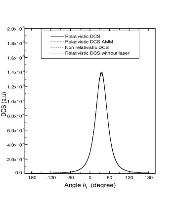
Figure 1: The various DCSs as a function of the angle $\theta_{f}$ in degrees for an electrical field strength of $\varepsilon=0.05$ $a.u$ and a relativistic parameter $\gamma=1.0053$. The corresponding number of photons exchanged is $\pm 1200$.

The effect of the AMM of the electron plays a key role for this behaviour. But this violation has to be ascertained by increasing the number $n$ of photons. For $n=\pm 1200$ photons, upwards, this violation is confirmed meaning that even at low kinetic incident energies and moderate field strength, the effect of the AMM of the electron begins to be distinguished even if this effect is small. For this number $n$ of photons the $\left(d\sigma/d\Omega_{f}\right)^{RL}_{AMM}$ is higher at the peak than the $\left(d\sigma/d\Omega_{f}\right)^{RNL}$ while $\left(d\sigma/d\Omega_{f}\right)^{NRL}$ and $\left(d\sigma/d\Omega_{f}\right)^{RL}$ are close to each other which was to be expected since in the non relativistic regime, spin effects are small. This is shown in Fig.1.
If we maintain the value of the relativistic parameter $\gamma=1.0053$ and we increase the value of the electric field strength $\varepsilon$ from $0.05$ $a.u$ to $0.1$ $a.u$, the violation of the pseudo sum-rule is still present while the difference between the $\left(d\sigma/d\Omega_{f}\right)^{RL}_{AMM}$ and the $\left(d\sigma/d\Omega_{f}\right)^{RL}$ is more pronounced compared to the previous case where $\varepsilon=0.05$ $a.u$. This is shown in Fig.2 where $n$ is also taken to have the value $\pm 1200$. At the peaks of the DCSs the difference between these two is roughly equal to $6$ percent.

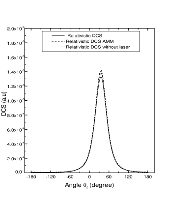
Figure 2: The various relativistic DCSs as a function of the angle $\theta_{f}$ in degrees for an electrical field strength of $\varepsilon=0.1$ $a.u$ and a relativistic parameter $\gamma=1.0053$. The corresponding number of photons exchanged is $\pm 1200$.

Figure 3: The various relativistic DCSs as a function of the angle $\theta_{f}$ in degrees for an electrical field strength of $\varepsilon=0.2$ $a.u$ and a relativistic parameter $\gamma=1.0053$. The corresponding number of photons exchanged is $\pm 1200$.

As the electric field strength is increased from $\varepsilon=0.1$ $a.u$ to $\varepsilon=0.2$ $a.u$, the physical insights mentioned are the same with a more noticeable difference between $\left(d\sigma/d\Omega_{f}\right)^{RL}_{AMM}$ and $\left(d\sigma/d\Omega_{f}\right)^{RL}$ of $36$ percent also at the peaks. This is shown in Fig.3.

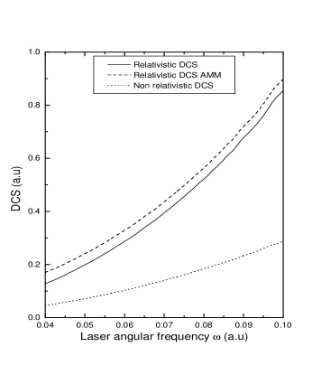
Figure 4: The various relativistic DCSs scaled in $10^{-5}$ as a function of $\omega$ for an electrical field strength of $\varepsilon=0.2$ $a.u$, a relativistic parameter $\gamma=1.0053$ and an angle $\theta_{f}=135^{\circ}$. The corresponding number of photons exchanged is $\pm 100$.

An interesting behaviour (with respect to the laser angular frequency $\omega$ varying from $0.04$ $a.u$ to $0.1$ $a.u$ and for $n=\pm 100$ photons in the non relativistic regime ($\gamma=1.0053$) and the same angular momentum coordinates) emerges with increasing $\varepsilon$, particularly for $\varepsilon=0.2$ $a.u$ where $\left(d\sigma/d\Omega_{f}\right)^{RL}_{AMM}$ is similar in shape as $\left(d\sigma/d\Omega_{f}\right)^{RL}$ but always higher. This advocates the fact that the term $1/2\sum_{s_{i}}\sum_{s_{f}}\left|M_{fi}^{(n)}\right|^{2}$ is very sensitive to the variation of $\varepsilon$ and this fact has to remain true for the relativistic regime. This is shown in Fig.4.
It is then necessary to ascertain this dependence with respect to the electric field strength by varying it from $\varepsilon=0.05$ $a.u$ to $\varepsilon=1$ $a.u$ while retaining all these same other parameters. From $\varepsilon=0.05$ $a.u$ to $\varepsilon=0.2$ $a.u$ the differences between the two interesting DCS are visible and begin to separate drastically up to $\varepsilon=1$ $a.u$ where, $\left(d\sigma/d\Omega_{f}\right)^{RL}_{AMM}\approx 11\left(d\sigma/d\Omega_{f}\right)^{RL}$.

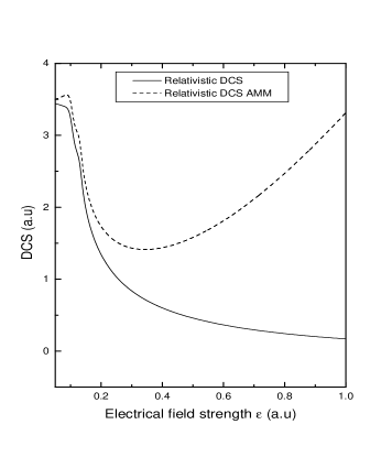
Figure 5: The two interesting DCSs scaled in $10^{-5}$ as a function of electrical field strength of $\varepsilon$ for a relativistic parameter $\gamma=1.0053$ and an angle $\theta_{f}=135^{\circ}$. The corresponding number of photons exchanged is $\pm 1000$.

Fig.5 clearly shows this behaviour as well as the strong dependence with respect to the electric field strength of $\left(d\sigma/d\Omega_{f}\right)^{RL}_{AMM}$.
Having given sound evidence of the role of the electric field strength, we now turn to the dynamical behaviour of the various DCSs with respect to the relativistic parameter $\gamma$ that is taken to vary from $\gamma=1.0053$ to $\gamma=1.025$ i.e maintaining the various simulations within the framework of the non relativistic regime. For $\varepsilon=0.05$ $a.u$ and $n=\pm 200$ the difference between the two relevant DCSs is small. This is also the case for $n=\pm 400$. Moreover, increasing $\varepsilon$ from $0.05$ $a.u$ to $0.1$ $a.u$ and fixing $n$ to vary between $\pm 1000$ gives a noticeable difference between the two commonly studied DCSs while at the same time confirming the violation of the pseudo sum-rule. This is shown in Fig.6.

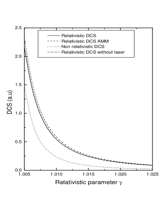
Figure 6: various DCSs scaled in $10^{-5}$ as a function of relativistic parameter $\gamma$ for an electrical field strength of $\varepsilon=0.1$ $a.u$ and an angle $\theta_{f}=135^{\circ}$. The corresponding number of photons exchanged is $\pm 1000$.

Two interesting comparisons can provide further physical insights concerning this process. The first one concerns the ratios $R_{1}=\ln(\left(\frac{d\sigma}{d\Omega_{f}}\right)^{RL}_{AMM}/\left(\frac{d\sigma}{d\Omega_{f}}\right)^{RNL})$ and $R_{2}=\ln(\left(\frac{d\sigma}{d\Omega_{f}}\right)^{RL}/\left(\frac{d\sigma}{d\Omega_{f}}\right)^{RNL})$. Maintaining the same geometry and the same values of $\varepsilon$ and $\gamma$ (that is $\varepsilon=0.05$ $a.u$ and $\gamma=1.0053$), the upper curve for $R_{1}$ is showing a minimum at the peak $\theta_{f}\approx 33^{\circ}$ and is neatly distinguishable from the second curve given by $R_{2}$. The fact that these two curves have their minima located at $\theta_{f}\approx 33^{\circ}$ is not surprising since they have been divided by $\left(d\sigma/d\Omega_{f}\right)^{RNL}$, that is the relativistic DCS without a laser field. Since we have taken the logarithm of the ratio of both DCS with an without AMM, the violation of the pseudo sum-rule is clearly visible in Fig. 7,namely for $R_{2}$. The behaviour of both ratios are nearly the same from negative values of $\theta_{f}$, meaning that for those angles, the contribution of the term $1/2\sum_{s_{i}}\sum_{s_{f}}\left|M_{fi}^{(n)}\right|^{2}$ has an overall effect of increasing $R_{1}$ compared to that of $R_{2}$ but the signature of the electron’s AMM is not important. Such a behaviour must be checked for the relativistic regime. Fig.7 gives the ratios $R_{1}$ and $R_{2}$.

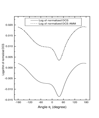
Figure 7: Logarithm of the relativistic DCS with AMM and relativistic DCS normalized to relativistic DCS without a laser field for an electrical field strength $\varepsilon=0.05$ $a.u$ and relativistic parameter $\gamma=1.0053$. The corresponding number of photons exchanged is $\pm 1200$.

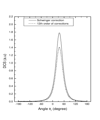
Figure 8: Comparison between DCS with AMM for Schwinger correction and 12th order of corrections, for an electrical field strength $\varepsilon=0.05$ $a.u$ and relativistic parameter $\gamma=1.0053$. The DCSs are scaled in $10^{-3}$ and the corresponding number of photons exchanged is $\pm 1000$.

To end this section concerning the non relativistic regime, one may ask whether the value used throughout this work for the electron’s anomaly is really sensitive to the order of the radiative corrections. This is indeed the case since Fig.8 shows that when using only the second order radiative correction found by Schwinger 2 , we have an over estimation for the $\left(d\sigma/d\Omega_{f}\right)^{RL}_{AMM}$(Schwinger) of about $28$ percent compared to the $\left(d\sigma/d\Omega_{f}\right)^{RL}_{AMM}$(12th order) meaning that radiative corrections reduce the values of the angular distributions. We have checked this for the same geometry and for $n=\pm 1000$ photons. Needless to say that such a comparison is out of our reach in the relativistic domain since the number $n$ must be very high to come with a convincing conclusion .

III.2 The relativistic regime.

The main difficulty when investigating the relativistic domain is the limitation due to the computing power of our computer (namely an intel (R) Core (TM) 2 DUO CPU 2.2 GHZ). Indeed, with such a material, it is not possible to go beyond a certain limit for $n$, the number of photons exchanged.
We have tried whenever this was possible, to extract qualitative results that will not change drastically when $n$ is increased.

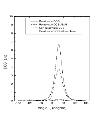
Figure 9: The various relativistic DCSs scaled in $10^{-8}$ as a function of the angle $\theta_{f}$ in degrees for an electrical field strength of $\varepsilon=1$ $a.u$ and a relativistic parameter $\gamma=2$. The corresponding number of photons exchanged is $\pm 5000$..

The angular parameters are the same as well as the laser frequency whereas $\varepsilon=1$ $a.u$ and $\gamma=2$.
The first physical quantities to be investigated are of course the various differential cross sections. Bearing in mind the limitation of our computer, we can’t go beyond a certain number of photons exchanged. The first observation that can be made concern the magnitudes of these DCSs that are strongly decreased in the relativistic regime. The dressed momentum coordinates ($\mathbf{q}_{i}$,$\mathbf{q}_{f}$) are now noticeably different from the non dressed momentum coordinates ($\mathbf{p}_{i}$,$\mathbf{p}_{f}$), therefore the maximum or peak of the various DCSs is now located at nearly $29$. In this regime, the differences between $\left(d\sigma/d\Omega_{f}\right)^{RL}_{AMM}$ and $\left(d\sigma/d\Omega_{f}\right)^{RL}$ are much more pronounced than those in the non relativistic regime and this was to be expected because there is a strong correlation between the electric field strength and the electron’s anomaly$\kappa$. Since the former one is increased from $\varepsilon=0.05$ $a.u$ to $\varepsilon=1$ $a.u$, the dependence of the DCSs are clearly shown in Fig.9.
This figure also shows that the overall behaviour of $\left(d\sigma/d\Omega_{f}\right)^{RL}_{AMM}$ .vs. $\left(d\sigma/d\Omega_{f}\right)^{RL}$ does not vary even with increasing values of $n$, we have then turned our investigation to an other aspect of the behaviour of a sole DCS with respect to the number of photons exchanged.
Fig.10 shows the increase of $\left(d\sigma/d\Omega_{f}\right)^{RL}$ for the different values of the summation over $n$, the first summation is over $n=\pm 1000$ photons while the last one is over $n=\pm 5000$ photons. Since the relativistic DCS without laser field is nearly $6.7510^{-8}$ at its maximum, it is obvious that one has to sum over a very large number of photons exchanged in order to obtain at least the $10^{-8}$ order of magnitude. Even for $n=\pm 5000$, the value of $\left(d\sigma/d\Omega_{f}\right)^{RL}$ is nearly $2.10^{-9}$ at its maximum. As there is linear relation between the summation over $n$ and the value of $\left(d\sigma/d\Omega_{f}\right)^{RL}$ at its peak, it is however possible to investigate this dependence by reducing the angular distribution interval.

Figure 10: The relativistic DCS with a laser field scaled in $10^{-10}$ for various values of number of photons exchanged, as a function of the angle $\theta_{f}$ in degrees for an electrical field strength of $\varepsilon=1$ $a.u$ and a relativistic parameter $\gamma=2$.

In Fig.11,

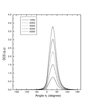
Figure 11: The relativistic DCS with AMM scaled in $10^{-8}$ for various values of number of photons exchanged, as a function of the angle $\theta_{f}$ in degrees for an electrical field strength of $\varepsilon=1$ $a.u$ and a relativistic parameter $\gamma=2$.

we show the same dependence of $\left(d\sigma/d\Omega_{f}\right)^{RL}_{AMM}$ and what emerges is a very different picture. Indeed, the value of this DCS at its maximum is now $4.10^{-8}$ for $n=\pm 5000$ which is close to the value of $\left(d\sigma/d\Omega_{f}\right)^{RL}$ at the same maximum. This means that we can, by reducing the angular distribution interval, investigate if there is violation of the pseudo sum rule as in the non relativistic regime. An interesting behaviour emerges when we vary the electrical field strength from $\varepsilon=0.05$ $a.u$ to $\varepsilon=1$ $a.u$. As $\gamma=2$, there is an interval of values of (0.05, 0.19) where there is a very weak quasi-linear decrease of $\left(d\sigma/d\Omega_{f}\right)^{RL}$ and this DCS decrease in a more pronounced manner in the interval (0.2, 0.3) while smoothly decreasing of other values of $\varepsilon$. This is consistent with the results shown in Fig.10-11 where the various DCSs have decreased values for $\gamma=2$ and $\varepsilon=1$ $a.u$. As for the quasilinear decrease of $\left(d\sigma/d\Omega_{f}\right)^{RL}$, the explanation is rather obvious since these values of $\varepsilon$ are in the vicinity of a ”quasi non relativistic” regime as far as we consider only $\varepsilon$. Indeed, considering the summation over $n$ ($\pm 20000$), this plateau-like behaviour means that we have reached and overtaken the required summation over $n$ for which the $\left(d\sigma/d\Omega_{f}\right)^{RL}$ converge to $\left(d\sigma/d\Omega_{f}\right)^{RNL}$.

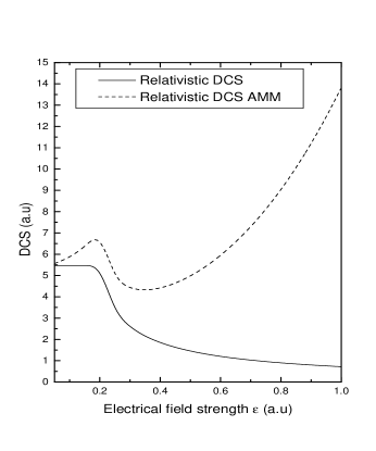
Figure 12: The two interesting DCSs scaled in $10^{-10}$ as a function of electrical field strength of $\varepsilon$ for a relativistic parameter $\gamma=2$ and an angle $\theta_{f}=135^{\circ}$. The corresponding number of photons exchanged is $\pm 20000$.

A contrasting behaviour is observed for $\left(d\sigma/d\Omega_{f}\right)^{RL}_{AMM}$ where we have summed as before over $\pm 20000$ photons. Even for $\gamma=2$, both DCSs remain close for small values of $\varepsilon$ typically ($0.05$,$0.075$) but begin to deviate from each other as $\varepsilon$ increase. A peak of $\left(d\sigma/d\Omega_{f}\right)^{RL}_{AMM}$ is present for $\varepsilon\simeq 0.19$ $a.u$ then there is a minimum for $\varepsilon\simeq 0.38$ $a.u$ and then a rapid increase for greater values of $\varepsilon$. The latter can be easily explained since the spinor part of $\left(d\sigma/d\Omega_{f}\right)^{RL}_{AMM}$ is strongly dependent on $\varepsilon$ as well as $\kappa$.
The first maximum and the next minimum are difficult to interpret since the expression of $\frac{1}{2}\sum_{s_{i}}\sum_{s_{f}}\left|M_{fi}^{(n)}\right|^{2}$ is very long and not prone to analytical investigation. However, since the angular parameters are fixed, $\gamma=2$, these can only be tracked back to the overall dependence of the spinor part of $\left(d\sigma/d\Omega_{f}\right)^{RL}_{AMM}$ on the electric field strength. These dependence with respect to $\varepsilon$ for both DCSs are shown in Fig.12.

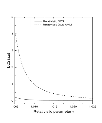
Figure 13: various DCSs scaled in $10^{-4}$ as a function of relativistic parameter $\gamma$ for an electrical field strength of $\varepsilon=1$ $a.u$ and an angle $\theta_{f}=135^{\circ}$. The corresponding number of photons exchanged is $\pm 10000$.

The relativistic effects on these DCSs can be investigated by varying the relativistic parameter $\gamma$. The number of photons exchanged is $\pm 10000$. But as we have $\varepsilon=1$ $a.u$, the interpretation of the curve obtained when $\gamma$ start from $1.005$ to the value $1.025$ must be cautiously carried out since there is an interplay between relativistic effect due to the variation of $\gamma$ and the fixed value of $\varepsilon$ on the one hand while on the other hand it does not give the whole picture of what really happens when $\gamma$ varies from $1.005$ to $2$. We have remedied to this computational task by studying three regions for the variation of $\gamma$, namely ($1.005$,$1.025$), ($1.495$,$1.505$), ($1.995$,$2$). An additional difficulty arises where varying $\gamma$ (while $\varepsilon$ remains fixed, $\varepsilon=1$ $a.u$), because both DCSs decrease by a factor of magnitude $4$ (from $\sim 10^{-4}$ to $10^{-8}$) when $\gamma$ approaches $2$. Therefore, even if $\left(d\sigma/d\Omega_{f}\right)^{RL}_{AMM}$ is always greater than $\left(d\sigma/d\Omega_{f}\right)^{RL}$, this cannot be visually translated in Fig.13. However, simulations for $\gamma\in(1.495,1.505)$ and $\gamma\in(1.995,2)$ give results that are consistent with previous ones. The effect of the frequency $\omega$ is shown in Fig.14 by varying $\omega$ from $0.04$ $a.u$ to $0.1$ $a.u$, for a relativistic parameter $\gamma=2$, an electric field strength $\varepsilon=1$ and for $n=\pm 10000$ photons. In this regime, the DCSs are not similar in shape as in the non relativistic regime ( see Fig.4). While both DCSs decrease in value (by an order of magnitude $3$), $\left(d\sigma/d\Omega_{f}\right)^{RL}$ is roughly quasi-linear whereas $\left(d\sigma/d\Omega_{f}\right)^{RL}_{AMM}$ decreases from its maximum value $7.510^{-10}$ ($a.u$) to a minimum located at $5.10^{-10}$ ($a.u$) and then increases.

Figure 14: The various relativistic DCSs scaled in $10^{-10}$ as a function of $\omega$ for an electrical field strength of $\varepsilon=1$ $a.u$, a relativistic parameter $\gamma=2$ and an angle $\theta_{f}=135^{\circ}$. The corresponding number of photons exchanged is $\pm 10000$.

IV Conclusion

In this work, we have presented new results concerning the effects of the electron’s anomalous magnetic moment on the process of laser-assisted electron-atomic hydrogen elastic collisions. We have used throughout this work the recent experimental value of the anomaly $a$ found by Gabrielse 3 . We have focused our study on the electronic dressing with the addition of the electron anomaly. Using the Dirac-Volkov wave function that incorporates this anomaly 18 , we found the analytical expression of the corresponding DCS. A spatial integral part that has been found in a previous work 21 remains the same for the study of this process. The various coefficients that intervene in the expression of $S_{fi}$ have been obtained using Reduce 22 . We have the same formal analogy between the DCS without and with anomaly. However, the spinor part incorporating this latter is strongly dependent on the electron’s anomaly and the electric field strength. For the non relativistic regime, the addition of the electron’s AMM is noticeable but small. When increasing the electric field strength to moderate values, this effect becomes more pronounced. For the first time, we have obtained the violation of the pseudo sum-rule 23 . We have also checked that the second order correction due to J. Schwinger 2 overestimates the DCS. In the relativistic regime, the dynamical behaviour of the DCS shows that the correlation between the terms stemming from the electron’s anomaly and the electric filed strength is more pronounced even if there is an overall decrease of DCS without electron’s anomaly and the DCS with the electron’s anomaly.

References

• (1) M. E. Peskin, D. V. Schroeder, An Introduction to Quantum Field Theory, Perseus Books Publishing, Reading, 1995.
• (2) J. Schwinger, Phys. Rev, 73, 416L (1948).
• (3) D. Hanneke, S. Fogwell and G. Gabrielse, Phys. Rev. Lett., 100, 120801 (2008).
• (4) E. Remiddi, Status of QED Predictions of the electron anomaly,INFN, Sezione di Bolognia, Frascati, 7 April 2008.
• (5) D. M. Volkov : Z. Phys. 94, 250 (1935).
• (6) J. San Roman, L. Plaja and L. Roso : Phys. Rev. A 64, 063402 (2001).
• (7) L.S. Brown and T.W.B. Kibble: Phys. Rev. 133, A705 (1964)
• (8) O. von Roos: Phys. Rev. 135, A43 (1964)
• (9) Z. Fried and J.H. Eberly: Phys. Rev. 136, B871 (1964)
• (10) T.W.B. Kibble: Phys. Rev. 150, 1060 (1966)
• (11) E.S. Sarachik and G.T. Schappert: Phys. Rev. D 1, 2738 (1970)
• (12) H. R. Reiss Editor, Focus Issue : Relativistic Effects in Strong Fields, Optics Express, Vol. 2, No. 7, 261 (1998).
• (13) T. Brabec Editor, Strong Field Laser Physics, Springer Series in Optical Sciences, Springer Science (2008).
• (14) E. Lötstedt, Laser-assisted second-order relativistic QED Processes : Bremsstrahlung and pair creation modified by a strong electromagnetic wave field , Thesis, University of Heidelberg, Germany (2008).
• (15) E. Lötstedt, U. D. Jentschura and C. H. Keitel Phys. Rev. Lett. 98, 043002 (2007).
• (16) S. Schnez, E. Lötstedt, U. D. Jentschura and C. H. Keitel Phys. Rev. A 75, 053412 (2007).
• (17) J. D. Bjorken, S. D. Drell, Relativistic Quantum Mechanics, McGraw-Hill Book Company, 1964.
• (18) Y. I. Salamin, J. Phys. A: Math. Gen., 26 6067-6071 (1993).
• (19) J. M. Djiokap, H. M. Tetchou Nganso and M. G. Kwato Njock, Phys. Scr., 75 726-733, 2007.
• (20) W. Greiner and J. Reinhardt, Quantum Electrodynamics, 3ed, Springer, 2003.
• (21) Y. Attaourti, B. Manaut and A. Makhoute, Phys. Rev. A, 69, 063407 (2004).
• (22) A. G. Grozin, Using Reduce in High Energy Physics( Cambridge University Press, 1997).
• (23) N. M. Kroll and K. M. Watson, Phys. Rev. A 8, 804 (1973).