Approximation by log-concave distributions, with applications to regression

Abstract

We study the approximation of arbitrary distributions $P$ on $d$-dimensional space by distributions with log-concave density. Approximation means minimizing a Kullback–Leibler-type functional. We show that such an approximation exists if and only if $P$ has finite first moments and is not supported by some hyperplane. Furthermore we show that this approximation depends continuously on $P$ with respect to Mallows distance $D_{1}(\cdot,\cdot)$. This result implies consistency of the maximum likelihood estimator of a log-concave density under fairly general conditions. It also allows us to prove existence and consistency of estimators in regression models with a response $Y=\mu(X)+\varepsilon$, where $X$ and $\varepsilon$ are independent, $\mu(\cdot)$ belongs to a certain class of regression functions while $\varepsilon$ is a random error with log-concave density and mean zero.

,
and

t1Supported by the Swiss National Science Foundation.

1 Introduction

Log-concave distributions, that is, distributions with a Lebesgue density the logarithm of which is concave, are an interesting nonparametric model comprising many parametric families of distributions. Bagnoli and Bergstrom (2005) give an overview of many interesting properties and applications in econometrics. Indeed, these distributions have received a lot of attention among statisticians recently as described in the review by Walther (2009). The nonparametric maximum likelihood estimator was studied in the univariate setting by Pal, Woodroofe and Meyer (2007), Rufibach (2006), Dümbgen, Hüsler and Rufibach (2007), Balabdaoui, Rufibach and Wellner (2009) and Dümbgen and Rufibach (2009). These references contain characterizations of the estimators, consistency results and explicit algorithms. Extensions of one or more of these aspects to the multivariate setting are presented by Cule, Samworth and Stewart (2010), Cule and Samworth (2010), Koenker and Mizera (2010), Seregin and Wellner (2010) and Schuhmacher and Dümbgen (2010). Both Cule and Samworth (2010) and Schuhmacher, Hüsler and Dümbgen (2009) show that multivariate log-concave distributions are a very well-behaved nonparametric class. For instance, moments of arbitrary order are continuous statistical functionals with respect to weak convergence.

The first aim of the present paper is a deeper understanding of the approximation scheme underlying the maximum likelihood estimator of a log-concave density. Let us put this into a somewhat broader context: let $\hat{Q}_{n}$ be the empirical distribution of independent random vectors $X_{1}$, $X_{2},\ldots,X_{n}$ with distribution $Q$ on a given open set $\mathcal{X}\subseteq\mathbb{R}^{d}$. Suppose that $Q$ has a density $f$ belonging to a given class $\mathcal{F}$ of probability densities on $\mathcal{X}$. The maximum likelihood estimator of $f$ may be written as

$$\hat{f}_{n}=\mathop{\arg\max}_{f\in\mathcal{F}}\int\log(f)\,d\hat{Q}_{n}$$

(provided this exists and is unique). Even if $Q$ fails to have a density within $\mathcal{F}$, one may view $\hat{f}_{n}$ as an estimator of the approximating density

$$f(\cdot|Q):=\mathop{\arg\max}_{f\in\mathcal{F}}\int\log(f)\,dQ.$$

In fact, if $Q$ has a density $g\notin\mathcal{F}$ on $\mathcal{X}$ such that the integral $\int g(x)\log g(x)\,dx$ exists in $\mathbb{R}$, one may rewrite $f(\cdot|Q)$ as the minimizer of the Kullback–Leibler divergence,

$$D_{\mathrm{KL}}(f,g)=\int\log(g/f)(x)g(x)\,dx,$$

over all $f\in\mathcal{F}$. Note the well-known fact that $D_{\mathrm{KL}}(f,g)>0$ unless $f=g$ almost everywhere. Viewing a maximum likelihood estimator as an estimator of an approximation within a given model is common in statistics [see, e.g., Pfanzagl (1990), Patilea (2001), Doksum et al. (2007) and Cule and Samworth (2010)]. Pfanzagl (1990) and Patilea (2001) show that under suitable regularity conditions on $Q$ and $\mathcal{F}$, the estimator $\hat{f}_{n}$ is consistent with certain large deviation bounds or rates of convergence, even in the case of misspecified models. To the best of our knowledge, their results are not directly applicable in the setting of log-concave densities, which is treated by Cule and Samworth (2010). Our ambition is to identify the largest possible class of distributions $Q$ such that $f(\cdot|Q)$ is well defined and unique. Moreover, we want to show that the mapping $Q\mapsto f(\cdot|Q)$ is continuous on that class with respect to a coarse topology, ideally the topology of weak convergence.

With these goals in mind, let us tell a short success story about Grenander’s estimator [Grenander (1956)], also a key example of Patilea (2001): let $\mathcal{F}_{\mathrm{mon}}$ be the class of all nonincreasing and left-continuous probability densities on $\mathcal{X}=(0,\infty)$. Then for any distribution $Q$ on $(0,\infty)$, the maximizer

$$f_{\mathrm{mon}}(\cdot|Q):=\mathop{\arg\max}_{f\in\mathcal{F}_{\mathrm{mon}}}\int_{(0,\infty)}\log f(x)Q(dx)$$

is well defined and unique. Namely, if $G$ denotes the distribution function of $Q$, then $f_{\mathrm{mon}}(\cdot|Q)$ is the left-sided derivative of the smallest concave majorant of $G$ on $(0,\infty)$ [see Barlow et al. (1972)]. With this characterization one can show that for any sequence of distributions $Q_{n}$ on $(0,\infty)$ converging weakly to $Q$,

$$\int_{(0,\infty)}\bigl{|}f_{\mathrm{mon}}(x|Q_{n})-f_{\mathrm{mon}}(x|Q)\bigr{|}\,dx\to 0\qquad(n\to\infty).$$

Since the sequence of empirical measures $\hat{Q}_{n}$ converges weakly to $Q$ almost surely, this entails strong consistency of the Grenander estimator $f(\cdot|\hat{Q}_{n})$ in total variation distance.

In the remainder of the present paper we consider the class $\mathcal{F}$ of log-concave probability densities on $\mathcal{X}=\mathbb{R}^{d}$. We will show in Section 2 that $f(\cdot|Q)$ exists and is unique in $L^{1}(\mathbb{R}^{d})$ if and only if

$$\int\|x\|Q(dx)<\infty$$

and

$$Q(H)<1\qquad\mbox{for any hyperplane }H\subset\mathbb{R}^{d}.$$

Some additional properties of $f(\cdot|Q)$ will be established as well. We show that the mapping $Q\mapsto f(\cdot|Q)$ is continuous with respect to Mallows distance [Mallows (1972)] $D_{1}(\cdot,\cdot)$, also known as a Wasserstein, Monge–Kantorovich or Earth Mover’s distance. Precisely, let $Q$ satisfy the properties just mentioned, and let $(Q_{n})_{n}$ be a sequence of probability distributions converging to $Q$ in $D_{1}$; in other words,

$$Q_{n}\to_{w}Q\quad\mbox{and}\quad\int\|x\|Q_{n}(dx)\to\int\|x\|Q(dx)$$ (1)

as $n\to\infty$. Then $f(\cdot|Q_{n})$ is well defined for sufficiently large $n$ and

$$\lim_{n\to\infty}\int\bigl{|}f(x|Q_{n})-f(x|Q)\bigr{|}\,dx=0.$$

This entails strong consistency of the maximum likelihood estimator $\hat{f}_{n}$, because $(\hat{Q}_{n})_{n}$ converges almost surely to $Q$ with respect to Mallows distance $D_{1}(\cdot,\cdot)$. In addition we show that $Q\mapsto\max_{f\in\mathcal{F}}\int\log(f)\,dQ$ is convex and upper semicontinuous with respect to weak convergence.

In Section 3 we apply these results to the following type of regression problem: suppose that we observe independent real random variables $Y_{1}$, $Y_{2},\ldots,Y_{n}$ such that

$$Y_{i}=\mu(x_{i})+\varepsilon_{i}$$

for given fixed design points $x_{1},x_{2},\ldots,x_{n}$ in some set $\mathcal{X}$, some unknown regression function $\mu\dvtx\mathcal{X}\to\mathbb{R}$ and independent, identically distributed random errors $\varepsilon_{i}$ with unknown log-concave density $f$ and mean zero. We will show that a maximum likelihood estimator of $(\mu,f)$ exists and is consistent under certain regularity conditions in the following two cases: (i) $\mathcal{X}=\mathbb{R}^{q}$ and $\mu$ is affine (i.e., affine linear); (ii) $\mathcal{X}=\mathbb{R}$ and $\mu$ is nondecreasing. These methods are illustrated with a real data set.

Many proofs and technical arguments are deferred to Section 4. A longer and more detailed version of this paper is the technical report by Dümbgen, Samworth and Schuhmacher (2010), referred to as [DSS 2010] hereafter. It contains all proofs, additional examples and plots, a detailed description of our algorithms and extensive simulation studies. There we also indicate potential applications to change-point analyses.

2 Log-concave approximations

For a fixed dimension $d\in\mathbb{N}$, let $\Phi=\Phi(d)$ be the family of concave functions $\phi\dvtx\mathbb{R}^{d}\to[-\infty,\infty)$ which are upper semicontinuous and coercive in the sense that

$$\phi(x)\to-\infty\qquad\mbox{as }\|x\|\to\infty.$$

In particular, for any $\phi\in\Phi$ there exist constants $a$ and $b>0$ such that $\phi(x)\leq a-b\|x\|$, so $\int e^{\phi(x)}\,dx$ is finite. Further let $\mathcal{Q}=\mathcal{Q}(d)$ be the family of all probability distributions $Q$ on $\mathbb{R}^{d}$. Then we define a log-likelihood-type functional

$$L(\phi,Q):=\int\phi\,dQ-\int e^{\phi(x)}\,dx+1$$

and a profile log-likelihood

$$L(Q):=\sup_{\phi\in\Phi}L(\phi,Q).$$

If, for fixed $Q$, there exists a function $\psi\in\Phi$ such that $L(\psi,Q)=L(Q)\in\mathbb{R}$, then it will automatically satisfy

$$\int e^{\psi(x)}\,dx=1.$$

To verify this, note that $\phi+c\in\Phi$ for any fixed function $\phi\in\Phi$ and arbitrary $c\in\mathbb{R}$, and

$$\frac{\partial}{\partial c}L(\phi+c,Q)=1-e^{c}\int e^{\phi(x)}\,dx,$$

if $L(\phi,Q)\in\mathbb{R}$. Thus $L(\phi+c,Q)$ is minimal for $c=-\log\int e^{\phi(x)}\,dx$.

2.1 Existence, uniqueness and basic properties

The next theorem provides a complete characterization of all distributions $Q\in\mathcal{Q}$ with real profile log-likelihood $L(Q)$. To state the result we first define the convex support of a distribution $Q\in\mathcal{Q}$ and collect some of its properties.

Lemma 2.1 ((DSS 2010))

For any $Q\in\mathcal{Q}$, the set

$$\operatorname{csupp}(Q):=\bigcap\{C\dvtx C\subseteq\mathbb{R}^{d}\mbox{ closed and convex},Q(C)=1\}$$

is itself closed and convex with $Q(\operatorname{csupp}(Q))=1$. The following three properties of $Q$ are equivalent:

[(a)]

$\operatorname{csupp}(Q)$ has nonempty interior;

$Q(H)<1$ for any hyperplane $H\subset\mathbb{R}^{d}$;

with $\operatorname{Leb}$ denoting Lebesgue measure on $\mathbb{R}^{d}$,

$$\lim_{\delta\downarrow 0}\sup\{Q(C)\dvtx C\subset\mathbb{R}^{d}\mbox{ closed and convex},\operatorname{Leb}(C)\leq\delta\}<1.$$

Theorem 2.2

For any $Q\in\mathcal{Q}$, the value of $L(Q)$ is real if and only if

$$\int\|x\|Q(dx)<\infty\quad\mbox{and}\quad\operatorname{interior}(\operatorname{csupp}(Q))\neq\varnothing.$$

In that case, there exists a unique function

$$\psi=\psi(\cdot|Q)\in\mathop{\arg\max}_{\phi\in\Phi}L(\phi,Q).$$

This function $\psi$ satisfies $\int e^{\psi(x)}\,dx=1$ and

$$\operatorname{interior}(\operatorname{csupp}(Q))\subseteq\operatorname{dom}(\psi):=\{x\in\mathbb{R}^{d}\dvtx\psi(x)>-\infty\}\subseteq\operatorname{csupp}(Q).$$

Remark 2.3 ([Moment (in)equalities]).

Let $Q\in\mathcal{Q}$ satisfy the properties stated in Theorem 2.2. Then the log-density $\psi=\psi(\cdot|Q)$ satisfies the following requirements: $L(\psi,Q)=\int\psi\,dQ\in\mathbb{R}$, and for any function $\Delta\dvtx\mathbb{R}^{d}\to\mathbb{R}$,

$$\int\Delta\,dQ\leq\int\Delta(x)e^{\psi(x)}\,dx\qquad\mbox{if }\psi+t\Delta\in\Phi\qquad\mbox{for some }t>0.$$ (2)

This follows from

$$\lim_{t\downarrow 0}t^{-1}\bigl{(}L(\psi+t\Delta,Q)-L(\psi,Q)\bigr{)}=\int\Delta\,dQ-\int\Delta(x)e^{\psi(x)}\,dx.$$

Let $P$ be the approximating probability measure with $P(dx)=e^{\psi(x)}\,dx$. It satisfies the following (in)equalities:

$$\int h\,dP \leq \int h\,dQ\qquad\mbox{for any convex }h\dvtx\mathbb{R}^{d}\to(-\infty,\infty],$$ (3)

$$\int xP(dx) = \int xQ(dx).$$ (4)

To verify (3), let $v\in\mathbb{R}^{d}$ be a subgradient of $h$ at $0$, that is, $h(x)\geq h(0)+v^{\top}x$ for all $x\in\mathbb{R}^{d}$. Since $\psi(x)\leq a-b\|x\|$ for arbitrary $x\in\mathbb{R}^{d}$ and suitable constants $a$ and $b>0$, the function $\Delta:=-h$ satisfies the requirement that $\psi+t\Delta\in\Phi$ whenever $0<t<b/\|v\|$. Hence the asserted inequality follows from (2). The equality for the first moments follows by setting $h(x):=\pm v^{\top}x$ for arbitrary $v\in\mathbb{R}^{d}$.

In what follows let

$$\mathcal{Q}^{1}=\mathcal{Q}^{1}(d) := \biggl{\{}Q\in\mathcal{Q}\dvtx\int\|x\|Q(dx)<\infty\biggr{\}},$$

$$\mathcal{Q}_{o}=\mathcal{Q}_{o}(d) := \{Q\in\mathcal{Q}\dvtx\operatorname{interior}(\operatorname{csupp}(Q))\neq\varnothing\}.$$

Thus $L(Q)\in\mathbb{R}$ if and only if $Q\in\mathcal{Q}_{o}\cap\mathcal{Q}^{1}$. Moreover, the proof of Theorem 2.2 shows that

$$L(Q)=\cases{-\infty,&\quad for $Q\in\mathcal{Q}\setminus\mathcal{Q}^{1}$,\cr+\infty,&\quad for $Q\in\mathcal{Q}^{1}\setminus\mathcal{Q}_{o}$.}$$

Remark 2.4 ((Affine equivariance)).

Suppose that $Q\in\mathcal{Q}_{o}\cap\mathcal{Q}^{1}$. For arbitrary vectors $a\in\mathbb{R}^{d}$ and nonsingular, real $d\times d$ matrices $B$ define $Q_{a,B}$ to be the distribution of $a+BX$ when $X$ has distribution $Q$. Then $Q_{a,B}\in\mathcal{Q}_{o}\cap\mathcal{Q}^{1}$, too, and elementary considerations reveal that

$$L(Q_{a,B})=L(Q)-{\log}|{\det B}|$$

and

$$\psi(x|Q_{a,B})=\psi\bigl{(}B^{-1}(x-a)|Q\bigr{)}-{\log}|{\det B}|\qquad\mbox{for }x\in\mathbb{R}^{d}.$$

Remark 2.5 ((Convexity, DSS 2010)).

The profile log-likelihood $L$ is convex on $\mathcal{Q}^{1}$. Precisely, for arbitrary $Q_{0},Q_{1}\in\mathcal{Q}^{1}$ and $0<t<1$,

$$L\bigl{(}(1-t)Q_{0}+tQ_{1}\bigr{)}\leq(1-t)L(Q_{0})+tL(Q_{1}).$$

The two sides are equal and real if and only if $Q_{0},Q_{1}\in\mathcal{Q}_{o}\cap\mathcal{Q}^{1}$ with $\psi(\cdot|Q_{0})=\psi(\cdot|Q_{1})$.

Remark 2.6 ((Concave majorants, DSS 2010)).

Let $\psi=\psi(\cdot|Q)$ for a distribution $Q\in\mathcal{Q}_{o}\cap\mathcal{Q}^{1}$. For any open set $U\subset\mathbb{R}^{d}$ there exists a (pointwise) minimal function $\psi_{U}\in\Phi$ such that $\psi_{U}\geq\psi$ on $\mathbb{R}^{d}\setminus U$. In particular, $\psi_{U}\leq\psi$ with equality on $\mathbb{R}^{d}\setminus U$. One can also show that $\psi_{U}$ is the pointwise infimum of all affine functions $\phi$ such that $\phi\geq\psi$ on $\mathbb{R}^{d}\setminus U$. If $\operatorname{supp}(Q)$ denotes the smallest closed set $A\subseteq\mathbb{R}^{d}$ with $Q(A)=1$, then

$$\psi=\psi_{\mathbb{R}^{d}\setminus\mathrm{supp}(Q)}.$$

Furthermore, suppose that $Q$ has a density $g$ on an open set $U$ such that $\psi>\log g$ on this set. Then

$$\psi=\psi_{U}.$$

2.2 The one-dimensional case

For the case of $d=1$ one can generalize Theorem 2.4 of Dümbgen and Rufibach (2009) as follows: for a function $\phi\in\Phi(1)$ let

$$\mathcal{S}(\phi):=\bigl{\{}x\in\operatorname{dom}(\phi)\dvtx\phi(x)>2^{-1}\bigl{(}\phi(x-\delta)+\phi(x+\delta)\bigr{)}\mbox{ for all }\delta>0\bigr{\}}.$$

The log-concave approximation of a distribution on $\mathbb{R}$ can be characterized in terms of distribution functions only:

Theorem 2.7

Let $Q$ be a nondegenerate distribution on $\mathbb{R}$ with finite first moment and distribution function $G$. Let $F$ be a distribution function with log-density $\phi\in\Phi$. Then $\phi=\psi(\cdot|Q)$ if and only if

$$\int_{-\infty}^{\infty}\bigl{(}F(t)-G(t)\bigr{)}\,dt=0$$

and

$$\int_{-\infty}^{x}\bigl{(}F(t)-G(t)\bigr{)}\,dt\cases{\leq 0,&\quad for all $x\in\mathbb{R}$,\cr=0,&\quad for all $x\in\mathcal{S}(\phi)$.}$$

Remark 2.8 ((DSS 2010)).

One consequence of this theorem is that the c.d.f. $F$ of $\psi(\cdot|Q)$ follows the c.d.f. $G$ of $Q$ quite closely in that

$$G(x-)\leq F(x)\leq G(x)\qquad\mbox{for arbitrary }x\in\mathcal{S}(\psi(\cdot|Q)).$$

Example 2.9.

Let $Q$ be a rescaled version of Student’s distribution $t_{2}$ with density and distribution function

$$g(x)=2^{-1}(1+x^{2})^{-3/2}\quad\mbox{and}\quad G(x)=2^{-1}\bigl{(}1+(1+x^{2})^{-1/2}x\bigr{)},$$

respectively. The best approximating log-concave distribution is the Laplace distribution with density and distribution function

$$f(x)=2^{-1}e^{-|x|}\quad\mbox{and}\quad F(x)=\cases{f(x),&\quad for $x\leq 0$,\cr 1-f(x),&\quad for $x\geq 0$,}$$

respectively. To verify this claim, note that by symmetry it suffices to show that

$$\int_{-\infty}^{x}\bigl{(}F(t)-G(t)\bigr{)}\,dt\cases{\leq 0,&\quad for $x\leq 0$,\cr=0,&\quad for $x=0$.}$$

Indeed the integral on the left-hand side equals

$$2^{-1}\bigl{(}\exp(x)-x-(1+x^{2})^{1/2}\bigr{)}$$

for all $x\leq 0$. Clearly this expression is zero for $x=0$, and elementary considerations show that it is nonpositive for all $x\leq 0$. Numerical calculations reveal that $|F-G|$ is smaller than $0.04$ everywhere.

Remark 2.10.

Let $Q\in\mathcal{Q}_{o}\cap\mathcal{Q}^{1}$ such that $Q(a,b)=0$ for some bounded interval $(a,b)\subset\operatorname{csupp}(Q)$. Then $\psi=\psi(\cdot|Q)$ is linear on $[a,b]$. This follows from Remark 2.6, applied to $U=(a,b)$. Note that $\psi(a)>-\infty$ and $\psi(b)>-\infty$, because otherwise $\psi\equiv-\infty$ on $(-\infty,a]$ or on $[b,\infty)$. But this would be incompatible with $\int\psi\,dQ\in\mathbb{R}$, because both $Q((-\infty,a])$ and $Q([b,\infty))$ are positive.

Remark 2.11 ((DSS 2010)).

Suppose that $Q$ has a continuous but not log-concave density $g$. Nevertheless one can say the following about the approximating log-density $\psi=\psi(\cdot|Q)$:

Suppose that $\log g$ is concave on an interval $(-\infty,a]$ with $g(a)>0$ and $\psi(a)\leq\log g(a)$. Then there exists a point $a^{\prime}\in[-\infty,a]$ such that $\psi$ is linear on $(a^{\prime},a]$ and $\psi=\log g$ on $(-\infty,a^{\prime}]$.

Suppose that $\log g$ is differentiable everywhere, convex on a bounded interval $[a,b]$ and concave on both $(-\infty,a]$ and $[b,\infty)$. Then there exist points $a^{\prime}\in(-\infty,a]$ and $b^{\prime}\in[b,\infty)$ such that $\psi$ is linear on $[a^{\prime},b^{\prime}]$ while $\psi=\log g$ on $(-\infty,a^{\prime}]\cup[b^{\prime},\infty)$.

Suppose that $\log g$ is convex on an interval $(-\infty,a]$ such that $-\infty<\log g(a)\leq\psi(a)$. Then $\psi$ is linear on $(-\infty,a]$.

Example 2.12.

Let us illustrate part (ii) of Remark 2.11 with a numerical example. Figure 1 shows the bimodal

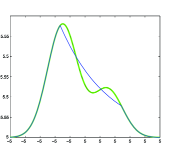
Figure 1: Density of a Gaussian mixture and its log-concave approximation.

density $g$ (green/dotted line) of the Gaussian mixture $Q=0.7\cdot\mathcal{N}(-1.5,1)+0.3\cdot\mathcal{N}(1.5,1)$ together with its log-concave approximation $f=f(\cdot|Q)$ (blue line). As predicted, there exists an interval $[a^{\prime},b^{\prime}]$ such that $f=g$ on $\mathbb{R}\setminus(a^{\prime},b^{\prime})$ and $\log f$ is linear on $[a^{\prime},b^{\prime}]$.

2.3 Continuity in $Q$

For the applications to regression problems to follow we need to understand the properties of both $Q\mapsto L(Q)$ and $Q\mapsto\psi(\cdot|Q)$ on $\mathcal{Q}^{1}\cap\mathcal{Q}_{o}$. Our first hope was that both mappings would be continuous with respect to the weak topology. It turned out, however, that we need a somewhat stronger notion of convergence, namely, convergence with respect to Mallows distance $D_{1}$ which is defined as follows: for two probability distributions $Q,Q^{\prime}\in\mathcal{Q}^{1}$,

$$D_{1}(Q,Q^{\prime}):=\inf_{(X,X^{\prime})}\mathbb{E}\|X-X^{\prime}\|,$$

where the infimum is taken over all pairs $(X,X^{\prime})$ of random vectors $X\sim Q$ and $X^{\prime}\sim Q^{\prime}$ on a common probability space. It is well known that the infimum in $D_{1}(Q,Q^{\prime})$ is a minimum. The distance $D_{1}$ is also known as Wasserstein, Monge–Kantorovich or Earth Mover’s distance. An alternative representation due to Kantorovič and Rubinšteĭn (1958) is

$$D_{1}(Q,Q^{\prime})=\sup_{h\in\mathcal{H}_{L}}\biggl{|}\int h\,dQ-\int h\,dQ^{\prime}\biggr{|},$$

where $\mathcal{H}_{L}$ consists of all $h\dvtx\mathbb{R}^{d}\to\mathbb{R}$ such that $|h(x)-h(y)|\leq\|x-y\|$ for all $x,y\in\mathbb{R}^{d}$. Moreover, for a sequence $(Q_{n})_{n}$ in $\mathcal{Q}^{1}$, it is known that (1) is equivalent to $D_{1}(Q_{n},Q)\to 0$ as $n\to\infty$ [Mallows (1972), Bickel and Freedman (1981)]. In case of $d=1$, the optimal coupling of $Q$ and $Q^{\prime}$ is given by the quantile transformation: if $G$ and $G^{\prime}$ denote the respective distribution functions, then

$$D_{1}(Q,Q^{\prime})=\int_{0}^{1}|G^{-1}(u)-{G^{\prime}}^{-1}(u)|\,du=\int_{-\infty}^{\infty}|G(x)-G^{\prime}(x)|\,dx.$$

A good starting point for more detailed information on Mallows distance is Chapter 7 of Villani (2003).

Before presenting the main results of this section we mention two useful facts about the convex support of distributions.

Lemma 2.13

Given a distribution $Q\in\mathcal{Q}$, a point $x\in\mathbb{R}^{d}$ is an interior point of $\operatorname{csupp}(Q)$ if and only if

$$h(Q,x):=\sup\{Q(C)\dvtx C\subset\mathbb{R}^{d}\mbox{ closed and convex},x\notin\operatorname{interior}(C)\}<1.$$

Moreover, if $(Q_{n})_{n}$ is a sequence in $\mathcal{Q}$ converging weakly to $Q$, then

$$\limsup_{n\to\infty}h(Q_{n},x)\leq h(Q,x)\qquad\mbox{for any }x\in\mathbb{R}^{d}.$$

This lemma implies that the set $\mathcal{Q}_{o}$ is an open subset of $\mathcal{Q}$ with respect to the topology of weak convergence. The supremum $h(Q,x)$ is a maximum over closed halfspaces and is related to Tukey’s halfspace depth [Donoho and Gasko (1992), Section 6]. For a proof of Lemma 2.13 we refer to [DSS 2010]. Now we are ready to state the main results of this section.

Theorem 2.14 ((Weak upper semicontinuity))

Let $(Q_{n})_{n}$ be a sequence of distributions in $\mathcal{Q}_{o}$ converging weakly to some $Q\in\mathcal{Q}_{o}$. Then

$$\limsup_{n\to\infty}L(Q_{n})\leq L(Q).$$

Moreover, $\liminf_{n\to\infty}L(Q_{n})<L(Q)$ if and only if

$$\limsup_{n\to\infty}\int\|x\|Q_{n}(dx)>\int\|x\|Q(dx).$$

This result already entails continuity of $L(\cdot)$ on $\mathcal{Q}_{o}\cap\mathcal{Q}^{1}$ with respect to Mallows distance $D_{1}$. The next theorem extends this result to $L\dvtx\mathcal{Q}^{1}\to(-\infty,\infty]$:

Theorem 2.15 ((Continuity with respect to Mallows distance $D_{1}$))

Let $(Q_{n})_{n}$ be a sequence of distributions in $\mathcal{Q}^{1}$ such that $\lim_{n\to\infty}D_{1}(Q_{n},Q)=0$ for some $Q\in\mathcal{Q}^{1}$. Then

$$\lim_{n\to\infty}L(Q_{n})=L(Q).$$

In case of $Q\in\mathcal{Q}_{o}\cap\mathcal{Q}^{1}$, the probability densities $f:=\exp\mbox{${}\circ{}$}\psi(\cdot|Q)$ and $f_{n}:=\exp\mbox{${}\circ{}$}\psi(\cdot|Q_{n})$ are well defined for sufficiently large $n$ and satisfy

$$\lim_{n\to\infty,x\to y}f_{n}(x) = f(y)\qquad\mbox{for all }y\in\mathbb{R}^{d}\setminus\partial\{f>0\},$$

$$\limsup_{n\to\infty,x\to y}f_{n}(x) \leq f(y)\qquad\mbox{for all }y\in\partial\{f>0\},$$

$$\lim_{n\to\infty}\int|f_{n}(x)-f(x)|\,dx = 0.$$

Remark 2.16 ((Stronger modes of convergence)).

The convergence of $(f_{n})_{n}$ to $f$ in total variation distance may be strengthened considerably. It follows from recent results of Cule and Samworth (2010) or Schuhmacher, Hüsler and Dümbgen (2009) that $(f_{n})_{n}\to f$ uniformly on arbitrary closed subsets of $\mathbb{R}^{d}\setminus\operatorname{disc}(f)$, where $\operatorname{disc}(f)$ is the set of discontinuity points of $f$. The latter set is contained in the boundary of the convex set $\{f>0\}$, hence a null set with respect to Lebesgue measure. Moreover, there exists a number $\varepsilon(f)>0$ such that

$$\lim_{n\to\infty}\int e^{\varepsilon(f)\|x\|}|f_{n}(x)-f(x)|\,dx=0.$$

More generally,

$$\lim_{n\to\infty}\int e^{A(x)}|f_{n}(x)-f(x)|\,dx=0$$

for any sublinear function $A\dvtx\mathbb{R}^{d}\to\mathbb{R}$ such that $\lim_{\|x\|\to\infty}e^{A(x)}f(x)=0$.

3 Applications to regression problems

Now we consider the regression setting described in the Introduction with observations $Y_{i}=\mu(x_{i})+\varepsilon_{i}$, $1\leq i\leq n$, where the $x_{i}\in\mathcal{X}$ are given fixed design points, $\mu\dvtx\mathcal{X}\to\mathbb{R}$ is an unknown regression function, and the $\varepsilon_{i}$ are independent random errors with mean zero and unknown distribution $Q$ on $\mathbb{R}$ such that $\psi=\psi(\cdot|Q)$ is well defined. The regression function $\mu$ is assumed to belong to a given family $\mathcal{M}$ with the property that

$$m+c\in\mathcal{M}\qquad\mbox{for arbitrary }m\in\mathcal{M},c\in\mathbb{R}.$$

3.1 Maximum likelihood estimation

We propose to estimate $(\psi,\mu)$ by a maximizer of

$$\hat{\Lambda}(\phi,m):=\frac{1}{n}\sum_{i=1}^{n}\phi\bigl{(}Y_{i}-m(x_{i})\bigr{)}-\int e^{\phi(x)}\,dx+1$$

over all $(\phi,m)\in\Phi\times\mathcal{M}$. Note that $\hat{\Lambda}(\phi,m)$ remains unchanged if we replace $(\phi,m)$ with $(\phi(\cdot+c),m+c)$ for an arbitrary $c\in\mathbb{R}$. For fixed $m$, the maximizer $\hat{\phi}=\hat{\phi}_{m}$ of $\hat{\Lambda}(\cdot,m)$ over $\Phi$ will automatically satisfy $\int\exp(\hat{\phi}(x))\,dx=1$ and $\int x\exp(\hat{\phi}(x))\,dx=n^{-1}\sum_{i=1}^{n}(Y_{i}-m(x_{i}))$. Thus if $(\hat{\phi},\hat{m})$ maximizes $\hat{\Lambda}(\cdot,\cdot)$ over $\Phi\times\mathcal{M}$, then

$$(\hat{\psi},\hat{\mu}):=\bigl{(}\hat{\phi}(\cdot+c),\hat{m}+c\bigr{)}\qquad\mbox{with }c:=\frac{1}{n}\sum_{i=1}^{n}\bigl{(}Y_{i}-\hat{m}(x_{i})\bigr{)}$$

maximizes $\hat{\Lambda}(\phi,m)$ over all $(\phi,m)\in\Phi\times\mathcal{M}$ satisfying the additional constraint that $\exp\mbox{${}\circ{}$}\phi$ defines a probability density with mean zero.

Define $\mathbf{x}:=(x_{i})_{i=1}^{n}$ and $m(\mathbf{x}):=(m(x_{i}))_{i=1}^{n}$. Then we may write

$$\hat{\Lambda}(\phi,m)=L\bigl{(}\phi,\hat{Q}_{m(\mathbf{x})}\bigr{)}$$

with the empirical distributions

$$\hat{Q}_{\mathbf{v}}:=\frac{1}{n}\sum_{i=1}^{n}\delta_{Y_{i}-v_{i}}$$

for $\mathbf{v}=(v_{i})_{i=1}^{n}\in\mathbb{R}^{n}$. Thus our procedure aims to find

$$(\hat{\phi},\hat{m})\in\mathop{\arg\max}_{(\phi,m)\in\Phi\times\mathcal{M}}L\bigl{(}\phi,\hat{Q}_{m(\mathbf{x})}\bigr{)},$$

and this representation is our key to proving the existence of $(\hat{\psi},\hat{\mu})$. Before doing so we state a simple inequality of independent interest, which follows from Jensen’s inequality and elementary considerations:

Lemma 3.1 ((DSS 2010))

For any distribution $Q\in\mathcal{Q}^{1}(1)$,

$$L(Q)\leq-\log\biggl{(}2\int|x-\operatorname{Med}(Q)|Q(dx)\biggr{)}\leq-\log\biggl{(}\int|x-\mu(Q)|Q(dx)\biggr{)},$$

where $\operatorname{Med}(Q)$ is a median of $Q$ while $\mu(Q)$ denotes its mean $\int xQ(dx)$.

Theorem 3.2 ((Existence in regression))

Suppose that the set $\mathcal{M}(\mathbf{x}):=\{m(\mathbf{x})\dvtx m\in\mathcal{M}\}\subset\mathbb{R}^{n}$ is closed and does not contain $\mathbf{Y}:=(Y_{i})_{i=1}^{n}$. Then there exists a maximizer $(\hat{\phi},\hat{m})$ of $\hat{\Lambda}(\phi,m)$ over all $(\phi,m)\in\Phi\times\mathcal{M}$.

The constraint $\mathbf{Y}\notin\mathcal{M}(\mathbf{x})$ excludes situations with perfect fit. In that case, the Dirac measure $\delta_{0}$ would be the most plausible error distribution.

Example 3.3 ((Linear regression)).

Let $\mathcal{X}=\mathbb{R}^{q}$, and let $\mathcal{M}$ consist of all affine functions on $\mathbb{R}^{q}$. Then $\mathcal{M}(\mathbf{x})$ is the column space of the design matrix

$$\mathbf{X}=\left[\matrix{1&1&\cdots&1\cr x_{1}&x_{2}&\cdots&x_{n}}\right]^{\top}\in\mathbb{R}^{n\times(q+1)},$$

hence a linear subspace of $\mathbb{R}^{n}$. Consequently there exists a maximizer $(\hat{\phi},\hat{m})$ of $\hat{\Lambda}$ over $\Phi\times\mathcal{M}$, unless $\mathbf{Y}\in\mathcal{M}(\mathbf{x})$.

Example 3.4 ((Isotonic regression)).

Let $\mathcal{X}$ be some interval on the real line, and let $\mathcal{M}$ consist of all isotonic functions $m\dvtx\mathcal{X}\to\mathbb{R}$. Then the set $\mathcal{M}(\mathbf{x})$ is a closed convex cone in $\mathbb{R}^{n}$. Here the condition that $\mathbf{Y}\notin\mathcal{M}(\mathbf{x})$ is equivalent to the existence of two indices $i,j\in\{1,2,\ldots,n\}$ such that $x_{i}\leq x_{j}$ but $Y_{i}>Y_{j}$.

Fisher consistency

The maximum likelihood estimator $(\hat{\psi},\hat{\mu})$ need not be unique in general. Nevertheless we will prove it to be consistent under certain regularity conditions. A key point here is Fisher consistency in the following sense: note that the expectation measure of the empirical distribution $\hat{Q}_{m(\mathbf{x})}$ equals

$$\mathbb{E}\hat{Q}_{m(\mathbf{x})}=\frac{1}{n}\sum_{i=1}^{n}Q\star\delta_{\mu(x_{i})-m(x_{i})}=Q\star R_{(\mu-m)(\mathbf{x})}$$

with

$$R_{\mathbf{v}}:=\frac{1}{n}\sum_{i=1}^{n}\delta_{v_{i}}.$$

But

$$L\bigl{(}Q\star R_{(\mu-m)(\mathbf{x})}\bigr{)}\leq L(Q)$$

with equality if and only if $\mu-m$ is constant on $\{x_{1},x_{2},\ldots,x_{n}\}$. This follows from a more general inequality which is somewhat reminiscent of Anderson’s lemma [Anderson (1955)]:

Theorem 3.5

Let $Q\in\mathcal{Q}_{o}(d)\cap\mathcal{Q}^{1}(d)$ and $R\in\mathcal{Q}^{1}(d)$. Then $Q\star R\in\mathcal{Q}_{o}\cap\mathcal{Q}^{1}$ and

$$L(Q\star R)\leq L(Q).$$

Equality holds if and only if $R=\delta_{a}$ for some $a\in\mathbb{R}^{d}$.

3.2 Consistency

In this subsection we consider a triangular scheme of independent observations $(x_{ni},Y_{ni})$, $1\leq i\leq n$, with fixed design points $x_{ni}\in\mathcal{X}_{n}$ and

$$Y_{ni}=\mu_{n}(x_{ni})+\varepsilon_{ni},$$

where $\mu_{n}$ is an unknown regression function in $\mathcal{M}_{n}$ and $\varepsilon_{n1},\varepsilon_{n2},\ldots,\varepsilon_{nn}$ are unobserved independent random errors with mean zero and unknown distribution $Q_{n}\in\mathcal{Q}_{o}(1)\cap\mathcal{Q}^{1}(1)$. Two basic assumptions are:

[(A.2)]

$\mathcal{M}_{n}(\mathbf{x}_{n})$ is a closed subset of $\mathbb{R}^{n}$ for every $n\in\mathbb{N}$;

$D_{1}(Q_{n},Q)\to 0$ for some distribution $Q\in\mathcal{Q}_{o}(1)\cap\mathcal{Q}^{1}(1)$.

We write $(\hat{\psi}_{n},\hat{\mu}_{n})$ for a maximizer of $L(\phi,\hat{Q}_{n,m})$ over all pairs $(\phi,m)\in\Phi\times\mathcal{M}_{n}$ such that $\int e^{\phi(x)}\,dx=1$ and $\int xe^{\phi(x)}\,dx=0$, where $\hat{Q}_{n,m}$ stands for the empirical distribution of the residuals $Y_{ni}-m(x_{ni})$, $1\leq i\leq n$. We also need to consider its expectation measure

$$Q_{n,m}:=\mathbb{E}\hat{Q}_{n,m}=Q_{n}\star R_{(\mu_{n}-m)(\mathbf{x}_{n})}.$$

Furthermore we write

$$\|\mathbf{v}\|_{n}:=\frac{1}{n}\sum_{i=1}^{n}|v_{i}|\qquad\mbox{for }\mathbf{v}=(v_{i})_{i=1}^{n}\in\mathbb{R}^{n}.$$

It is also convenient to metrize weak convergence. In Theorem 3.6 below we utilize the bounded Lipschitz distance: for probability distributions $Q,Q^{\prime}$ on the real line let

$$D_{\mathrm{BL}}(Q,Q^{\prime}):=\sup_{h\in\mathcal{H}_{\mathrm{BL}}}\biggl{|}\int h\,d(Q-Q^{\prime})\biggr{|},$$

where $\mathcal{H}_{\mathrm{BL}}$ is the family of all functions $h\dvtx\mathbb{R}\to[-1,1]$ such that $|h(x)-h(y)|\leq|x-y|$ for all $x,y\in\mathbb{R}$.

Theorem 3.6 ((Consistency in regression))

Let assumptions (A.1) and (A.2) be satisfied. Suppose further that: [(A.2)]

for arbitrary fixed $c>0$,

$$\sup_{m\in\mathcal{M}_{n}\dvtx\|(m-\mu_{n})(\mathbf{x}_{n})\|_{n}\leq c}D_{\mathrm{BL}}(\hat{Q}_{n,m},Q_{n,m})\to_{p}0.$$

Then, with $f_{n}:=\exp\mbox{${}\circ{}$}\psi(\cdot|Q_{n})$ and $\hat{f}_{n}:=\exp\mbox{${}\circ{}$}\hat{\psi}_{n}$, the maximum likelihood estimator $(\hat{f}_{n},\hat{\mu}_{n})$ of $(f_{n},\mu_{n})$ exists with asymptotic probability one and satisfies

$$\int|\hat{f}_{n}(x)-f_{n}(x)|\,dx\to_{p}0,\qquad\|(\hat{\mu}_{n}-\mu_{n})(\mathbf{x}_{n})\|_{n}\to_{p}0.$$

We know already that assumption (A.1) is satisfied for multiple linear regression and isotonic regression. Assumption (A.2) is a generalization of assuming a fixed error distribution for all sample sizes. The crucial point, of course, is assumption (A.3). In our two examples it is satisfied under mild conditions:

Theorem 3.7 ((Linear regression))

Let $\mathcal{M}_{n}$ be the family of all affine functions on $\mathcal{X}_{n}:=\mathbb{R}^{q(n)}$. If assumption (A.2) is satisfied, then (A.3) follows from

$$\lim_{n\to\infty}q(n)/n=0.$$

Theorem 3.8 ((Isotonic regression))

Let $\mathcal{M}_{n}$ be the set of all nondecreasing functions on an interval $\mathcal{X}_{n}\subseteq\mathbb{R}$. If assumption (A.2) holds true, then (A.3) follows from

$$\|\mu_{n}(\mathbf{x}_{n})\|_{n}=O(1).$$

The proof of Theorem 3.7 is given in Section 4. For the proof of Theorem 3.8, which uses similar ideas and an additional approximation argument, we refer to [DSS 2010].

3.3 Algorithms and numerical results

Computing the maximum likelihood estimator $(\hat{\psi},\hat{\mu})$ from Section 3.1 turns out to be a rather difficult task, because the function $\hat{\Lambda}$ can have multiple local maxima. In [DSS 2010] we discuss strengths and weaknesses of three different algorithms, including an alternating and a stochastic search algorithm. The third procedure, which is highly successful in the case of linear regression, is global maximization of the profile log-likelihood $\hat{\Lambda}(\theta):=\max_{\phi\in\Phi}\hat{\Lambda}(\phi,m_{\theta})$, where $m_{\theta}(x)=\theta^{\top}x$ for every $x\in\mathbb{R}^{q}$, by means of differential evolution [Price, Storn and Lampinen (2005)].

Extensive simulation studies in [DSS 2010] suggest that $(\hat{\psi},\hat{\mu})$ provides rather accurate estimates even if $n$ is only moderately large. For various skewed error distributions, $\hat{\mu}$ may be considerably better than the corresponding least squares estimator. As an example consider the simple linear regression model with observations

$$Y_{i}=c+\theta X_{i}+\varepsilon_{i},\qquad 1\leq i\leq n:=100,$$

where $X_{1},\ldots,X_{n}$ are independent design points from the $\operatorname{Unif}[0,3]$ distribution and $\varepsilon_{1},\ldots,\varepsilon_{n}$ are independent errors from a centered gamma distribution with shape parameter $r$ and variance $1$. Note that the distribution of $(\hat{\psi},\hat{\theta}-\theta)$ does not depend on $c$ or $\theta$. Monte Carlo estimation of the root mean squared error based on 1000 simulations of this model gives 0.023 for the estimator $\hat{\theta}$ versus 0.118 for the least squares estimator of $\theta$ if $r=1$, and 0.095 versus 0.113 for the same comparison if $r=3$.

3.4 A data example

A familiar task in econometrics is to model expenditure ($Y$) of households as a function of their income ($X$). Not only the mean curve (Engel curve) but also quantile curves play an important role. A related application are growth charts in which, for instance, $X$ is the age of a newborn or infant and $Y$ is its height or weight.

We applied our methods to a survey of $n=7125$ households in the United Kingdom in 1973 (data courtesy of W. Härdle, HU Berlin). The two variables we considered were annual income ($X_{\mathrm{raw}}$) and annual expenditure for food ($Y_{\mathrm{raw}}$). Figure 2 shows scatter plots of the raw and log-transformed data. To enhance visibility we only show a random subsample of size $n^{\prime}=1000$. In addition, isotonic quantile curves $x\mapsto\hat{q}_{\beta}(x)$ are added for $\beta=0.1$, $0.25$, $0.5$, $0.75$, $0.9$ (based on all observations). These pictures show clearly that the raw data are heteroscedastic, whereas for the log-transformed data, $(X_{i},Y_{i})=(\log_{10}X_{{\mathrm{raw}},i},\log_{10}Y_{{\mathrm{raw}},i})$, an additive model seems appropriate.

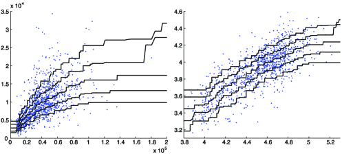
Figure 2: UK household data, raw (left) and log-transformed (right), with isotonic quantile curves.

Interestingly, neither linear nor quadratic nor cubic regression yield convincing fits to these data. Polynomial regression of degree four or cubic splines with knot points at, say, $4.1$, $4.3$, $4.5$, $4.7$, $4.9$ seem to fit the data quite well. Moreover, exact Monte Carlo goodness-of-fits test, assuming the regression function to be a cubic spline and based on a Kolmogorov–Smirnov statistic applied to studentized residuals, revealed the regression errors $\varepsilon_{i}$ to be definitely non-Gaussian.

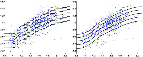
Figure 3: Log-transformed UK household data with isotonic fits (left) and spline fits (right) from our additive model.

Figure 3 shows the data and estimated $\beta$-quantile curves for $\beta=0.1$, $0.25$, $0.5$, $0.75$, $0.9$, based on our additive regression model. Note that the estimated $\beta$-quantile curve is simply the estimated mean curve plus the $\beta$-quantile of the estimated error distribution. On the left-hand side, we only assumed $\mu$ to be nondecreasing, on the right-hand side we fitted the aforementioned spline model. In both cases the fitted quantile curves are similar to the quantile curves in Figure 2 but with fewer irregularities such as big jumps which may be artifacts due to sampling error.

4 Proofs

For the proof of Theorem 2.2 we need an elementary bound for the Lebesgue measure of level sets of log-concave distributions:

Lemma 4.1 ((DSS 2010))

Let $\phi\in\Phi$ be such that $\int e^{\phi(x)}\,dx=1$. For real $t$ define the level set $D_{t}:=\{x\in\mathbb{R}^{d}\dvtx\phi(x)\geq t\}$. Then for $r<M\leq\max_{x\in\mathbb{R}^{d}}\phi(x)$,

$$\operatorname{Leb}(D_{r})\leq(M-r)^{d}e^{-M}\Big{/}\int_{0}^{M-r}t^{d}e^{-t}\,dt.$$

Another key ingredient for the proofs of Theorems 2.2 and 2.15 is a lemma on pointwise limits of sequences in $\Phi$:

Lemma 4.2 ((DSS 2010))

Let $\bar{\phi}$ and $\phi_{1},\phi_{2},\phi_{3},\ldots$ be functions in $\Phi$ such that $\phi_{n}\leq\bar{\phi}$ for all $n\in\mathbb{N}$. Further suppose that the set

$$C:=\Bigl{\{}x\in\mathbb{R}^{d}\dvtx\liminf_{n\to\infty}\phi_{n}(x)>-\infty\Bigr{\}}$$

is nonempty. Then there exist a subsequence $(\phi_{n(k)})_{k}$ of $(\phi_{n})_{n}$ and a function $\phi\in\Phi$ such that $C\subseteq\operatorname{dom}(\phi)=\{\phi>-\infty\}$ and

$$\lim_{k\to\infty,x\to y}\phi_{n(k)}(x) = \phi(y)\qquad\mbox{for all }y\in\operatorname{interior}(\operatorname{dom}(\phi)),$$

$$\limsup_{k\to\infty,x\to y}\phi_{n(k)}(x) \leq \phi(y)\leq\bar{\phi}(y)\qquad\mbox{for all }y\in\mathbb{R}^{d}.$$

Proof of Theorem 2.2 Suppose first that $\int\|x\|Q(dx)=\infty$. Since any $\phi\in\Phi$ is majorized by $x\mapsto a-b\|x\|$ for suitable constants $a$ and $b>0$, this entails that $L(Q)=-\infty$.

Second, suppose that $\int\|x\|Q(dx)<\infty$ but $\operatorname{interior}(\operatorname{csupp}(Q))=\varnothing$. According to Lemma 2.1, the latter fact is equivalent to $Q(H)=1$ for some hyperplane $H\subset\mathbb{R}^{d}$. For $c\in\mathbb{R}$ define a function $\phi_{c}\in\Phi$ via $\phi_{c}(x):=c-\|x\|$ for $x\in H$ and $\phi_{c}(x):=-\infty$ for $x\notin H$. Then $L(\phi_{c},Q)=c-\int\|x\|Q(dx)+1\to\infty$ as $c\to\infty$.

For the remainder of this proof suppose that $\int\|x\|Q(dx)<\infty$ and that $\operatorname{csupp}(Q)$ has nonempty interior. Since the concave function $h(x)=-\|x\|$ satisfies $\int h\,dQ>-\infty$, we have $L(Q)>-\infty$. When maximizing $L(\phi,Q)$ over all $\phi\in\Phi$ we may and do restrict our attention to functions $\phi\in\Phi$ such that $\int e^{\phi(x)}\,dx=1$ (see end of Section 1) and $\operatorname{dom}(\phi)=\{\phi>-\infty\}\subseteq\operatorname{csupp}(Q)$. For if $\operatorname{dom}(\phi)\not\subset\operatorname{csupp}(Q)$, replacing $\phi(x)$ with $-\infty$ for all $x\notin\operatorname{csupp}(Q)$ would also increase $L(\phi,Q)$ strictly. Let $\Phi(Q)$ be the family of all $\phi\in\Phi$ with these properties.

Now we show that $L(Q)<\infty$. Suppose that $\phi\in\Phi(Q)$ is such that $M:=\max_{x\in\mathbb{R}^{d}}\phi(x)>0$. With $D_{t}:=\{\phi\geq t\}$ and for $c>0$ we get the bound

$$L(\phi,Q) = \int\phi\,dQ\leq-cMQ(\mathbb{R}^{d}\setminus D_{-cM})+MQ(D_{-cM})$$

$$= -(c+1)M\biggl{(}\frac{c}{c+1}-Q(D_{-cM})\biggr{)}.$$

According to Lemma 4.1,

$$\operatorname{Leb}(D_{-cM}) \leq (1+c)^{d}M^{d}e^{-M}\Big{/}\int_{0}^{(1+c)M}t^{d}e^{-t}\,dt$$

$$= (1+c)^{d}M^{d}e^{-M}/\bigl{(}d!+o(1)\bigr{)}\to 0$$

as $M\to\infty$ for any fixed $c>0$. But Lemma 2.1 entails that for sufficiently large $c$ and sufficiently small $\delta>0$,

$$\sup\{Q(C)\dvtx C\subset\mathbb{R}^{d}\mbox{ closed and convex},\operatorname{Leb}(C)\leq\delta\}<\frac{c}{c+1},$$

whence

$$L(\phi,Q)\to-\infty\qquad\mbox{as }\max_{x\in\mathbb{R}^{d}}\phi(x)\to\infty.$$

Note also that $L(\phi,Q)\leq\max_{x\in\mathbb{R}^{d}}\phi(x)$ for any $\phi\in\Phi(Q)$. These considerations show that $L(Q)$ is finite and, for suitable constants $M_{o}<M_{*}$, equals the supremum of $L(\phi,Q)$ over all $\phi\in\Phi(Q)$ such that $M_{o}\leq\max_{x}\phi(x)\leq M_{*}$.

Next we show the existence of a maximizer $\phi\in\Phi(Q)$ of $L(\cdot,Q)$. Let $(\phi_{n})_{n}$ be a sequence of functions in $\Phi(Q)$ such that $-\infty<L(\phi_{n},Q)\uparrow L(Q)$ as $n\to\infty$, where $M_{n}:=\max_{x\in\mathbb{R}^{d}}\phi_{n}(x)\in[M_{o},M_{*}]$ for all $n\geq 1$. Now we show that

$$\inf_{n\geq 1}\phi_{n}(x_{o})>-\infty\qquad\mbox{for any }x_{o}\in\operatorname{interior}(\operatorname{csupp}(Q)).$$ (5)

If $\phi_{n}(x_{o})<M_{n}$, then $x_{o}$ is not an interior point of the closed, convex set $\{\phi_{n}\geq\phi_{n}(x_{o})\}$. Hence

$$\int\phi_{n}\,dQ \leq \phi_{n}(x_{o})+\bigl{(}M_{n}-\phi_{n}(x_{o})\bigr{)}Q\{\phi_{n}\geq\phi_{n}(x_{o})\}$$

$$\leq \phi_{n}(x_{o})+\bigl{(}M_{n}-\phi_{n}(x_{o})\bigr{)}h(Q,x_{o})$$

$$\leq \phi_{n}(x_{o})\bigl{(}1-h(Q,x_{o})\bigr{)}+\max(M_{n},0)$$

with $h(Q,x_{o})<1$ defined in Lemma 2.13. In the case of $\phi_{n}(x_{o})=M_{n}$ these inequalities are true as well. Thus

$$\phi_{n}(x_{o})\geq-\frac{\max(M_{n},0)-L(\phi_{n},Q)}{1-h(Q,x_{o})}\geq-\frac{\max(M_{*},0)-L(\phi_{1},Q)}{1-h(Q,x_{o})},$$

which establishes (5). Combining (5) with $\phi_{n}\leq M_{*}$, we may deduce from Lemma 3.3 of Schuhmacher, Hüsler and Dümbgen (2009) that there exist constants $a$ and $b>0$ such that

$$\phi_{n}(x)\leq a-b\|x\|\qquad\mbox{for all }n\in\mathbb{N},x\in\mathbb{R}^{d}.$$ (6)

The inequalities (5) and (6) and Lemma 4.2 with $C\supset\operatorname{interior}(\operatorname{csupp}(Q))$ and $\bar{\phi}(x):=a-b\|x\|$ imply existence of a function $\psi\in\Phi$ and a subsequence $(\phi_{n(k)})_{k}$ of $(\phi_{n})_{n}$ such that $\psi=-\infty$ on $\mathbb{R}^{d}\setminus\operatorname{csupp}(Q)$ and

$$\limsup_{k\to\infty}\phi_{n(k)}(x) \leq \psi(x)\leq a-b\|x\|\qquad\mbox{for all }x\in\mathbb{R}^{d},$$

$$\lim_{k\to\infty}\phi_{n(k)}(x) = \psi(x)>-\infty\qquad\mbox{for all }x\in\operatorname{interior}(\operatorname{csupp}(Q)).$$

Since the boundary of $\operatorname{csupp}(Q)$ has Lebesgue measure zero, it follows from dominated convergence that $\int e^{\psi(x)}\,dx=1$. Moreover, applying Fatou’s lemma to the nonnegative functions $x\mapsto a-b\|x\|-\phi_{n(k)}(x)$ yields

$$\limsup_{k\to\infty}\int\phi_{n(k)}\,dQ\leq\int\psi\,dQ.$$

Hence

$$L(Q)\geq L(\psi,Q)\geq\limsup_{k\to\infty}L\bigl{(}\phi_{n(k)},Q\bigr{)}=L(Q)$$

and thus $L(\psi,Q)=L(Q)$.

Uniqueness of the maximizer $\psi$ follows essentially from strict convexity of the exponential function: if $\tilde{\psi}\in\Phi(Q)$ with $L(\tilde{\psi},Q)>-\infty$, then $L((1-t)\psi+t\tilde{\psi},Q)$ is strictly concave in $t\in[0,1]$, unless $\operatorname{Leb}\{\psi\neq\tilde{\psi}\}=0$. But for $\psi,\tilde{\psi}\in\Phi(Q)$, the latter requirement is equivalent to $\psi=\tilde{\psi}$ everywhere.

In our proofs of Theorems 2.7 and 2.15 we utilize a special approximation scheme for functions in $\Phi$:

Lemma 4.3 ((DSS 2010))

For any function $\phi\in\Phi$ with nonempty domain and any parameter $\varepsilon>0$ set

$$\phi^{(\varepsilon)}(x):=\inf_{(v,c)}(v^{\top}x+c)$$

with the infimum taken over all $(v,c)\in\mathbb{R}^{d}\times\mathbb{R}$ such that $\|v\|\leq\varepsilon^{-1}$ and $\phi(y)\leq v^{\top}y+c$ for all $y\in\mathbb{R}^{d}$. This defines a function $\phi^{(\varepsilon)}\in\Phi$ which is real-valued and Lipschitz-continuous with constant $\varepsilon^{-1}$. Moreover, it satisfies $\phi^{(\varepsilon)}\geq\phi$ with equality if and only if $\phi$ is real-valued and Lipschitz-continuous with constant $\varepsilon^{-1}$. In general, $\phi^{(\varepsilon)}\downarrow\phi$ pointwise as $\varepsilon\downarrow 0$.

Proof of Theorem 2.7 Let $P$ be the distribution corresponding to $F$. Suppose first that $\phi=\psi(\cdot|Q)$. Then it follows from (4) and Fubini’s theorem that

$$0 = \int_{\mathbb{R}}x(Q-P)(dx)$$

$$= \int_{\mathbb{R}}\int_{\mathbb{R}}(1\{0<t<x\}-1\{x\leq t\leq 0\})\,dt(Q-P)(dx)$$

$$= \int_{\mathbb{R}}\bigl{(}1\{0<t\}(F-G)(t)-1\{t\leq 0\}(G-F)(t)\bigr{)}\,dt$$

$$= \int_{\mathbb{R}}(F-G)(t)\,dt.$$

Moreover, for any $x\in\mathbb{R}$, the function $s\mapsto(s-x)^{+}$ is convex so that (3) and Fubini’s theorem yield

$$0\leq\int_{\mathbb{R}}(s-x)^{+}(Q-P)(ds)=-\int_{-\infty}^{x}(F-G)(t)\,dt.$$

It remains to be shown that $\int_{-\infty}^{x}(F-G)(t)\,dt\geq 0$ for $x\in\mathcal{S}(\phi)$. Suppose first that $x\in\operatorname{interior}(\operatorname{dom}(\phi))$. Note that $\phi^{\prime}:=\phi^{\prime}(\cdot+)$ is nonincreasing on the interior of $\operatorname{dom}(\phi)$ with

$$\phi(x_{2})-\phi(x_{1})=\int_{x_{1}}^{x_{2}}\phi^{\prime}(u)\,du\qquad\mbox{for }x_{1},x_{2}\in\operatorname{interior}(\operatorname{dom}(\phi))\mbox{ with }x_{1}<x_{2}.$$

Moreover, $x\in\mathcal{S}(\phi)$ implies that $\phi^{\prime}(x-\delta)>\phi^{\prime}(x+\delta)$ for all $\delta>0$ satisfying $x\pm\delta\in\operatorname{interior}(\operatorname{dom}(\phi))$. For such $\delta>0$ we define

$$H_{\delta}(s):=\int_{-\infty}^{s}H_{\delta}^{\prime}(u)\,du$$

with

$$H_{\delta}^{\prime}(u):=\cases{0,&\quad\mbox{for} $u\leq x-\delta$,\vspace*{2pt}\cr\dfrac{\phi^{\prime}(x-\delta)-\phi^{\prime}(u)}{\phi^{\prime}(x-\delta)-\phi^{\prime}(x+\delta)},&\quad for $x-\delta<u\leq x+\delta$,\vspace*{2pt}\cr 1,&\quad for $u\geq x+\delta$.}$$

One can easily verify that $\phi+tH_{\delta}$ is upper semicontinuous and concave whenever $0<t\leq\phi^{\prime}(x-\delta)-\phi^{\prime}(x+\delta)$. In case of $t<-\inf_{u\in\mathbb{R}}\phi^{\prime}(u)$ it is also coercive. Thus it follows from (2) that

$$0 \leq \int_{\mathbb{R}}H_{\delta}(s)(P-Q)(ds)\to\int_{\mathbb{R}}(s-x)^{+}(P-Q)(ds)\qquad(\delta\downarrow 0)$$

$$= \int_{-\infty}^{x}(F-G)(t)\,dt.$$

When $x\in\mathcal{S}(\phi)$ is the left or right endpoint of $\operatorname{dom}(\phi)$, we define $\Delta(s):=(s-x)^{+}$ and conclude analogously that $\int_{-\infty}^{x}(F-G)(t)\,dt\geq 0$.

Now suppose that the distribution function $F$ with log-density $\phi\in\Phi$ satisfies the integral (in)equalities stated in Theorem 2.7. Let $\Delta\dvtx\mathbb{R}\to\mathbb{R}$ be Lipschitz-continuous with constant $L$, so for arbitrary $x,y\in\mathbb{R}$ with $x<y$,

$$\Delta(y)-\Delta(x)=\int_{x}^{y}\Delta^{\prime}(t)\,dt$$

with $\Delta^{\prime}\dvtx\mathbb{R}\to[-L,L]$ measurable. Then

$$\int\Delta d(Q-P)=\int_{\mathbb{R}}\Delta^{\prime}(t)(F-G)(t)\,dt.$$

Since $\int(F-G)(t)\,dt=0$, we may continue with

$$\int\Delta d(Q-P) = \int_{\mathbb{R}}\bigl{(}\Delta^{\prime}(t)+L\bigr{)}(F-G)(t)\,dt$$

$$= \int_{\mathbb{R}}\int_{-L}^{L}1\{s<\Delta^{\prime}(t)\}\,ds(F-G)(t)\,dt$$

$$= \int_{-L}^{L}\int_{A(\Delta^{\prime},s)}(F-G)(t)\,dt\,ds$$

with $A(\Delta^{\prime},s):=\{t\in\mathbb{R}\dvtx\Delta^{\prime}(t)>s\}$. Now we apply this representationto the function $\Delta:=\phi^{(\varepsilon)}$ for some $\varepsilon>0$, that is, $L=\varepsilon^{-1}$. Here one can show that $A(\Delta^{\prime},s)$ equals either $\varnothing$ or $\mathbb{R}$ or a half-line with right endpoint $a(\phi,s)=\min\{t\in\mathbb{R}\dvtx\phi^{\prime}(t+)\leq s\}$. But this entails that $a(\phi,s)\in\mathcal{S}(\phi)$, whence $\int_{A(\Delta^{\prime},s)}(F-G)(t)\,dt=0$ for all $s\in(-L,L)$. Consequently,

$$\int\phi^{(\varepsilon)}\,d(Q-P)=0.$$

If we consider $\Delta:=\psi^{(\varepsilon)}$ with $\psi:=\psi(\cdot|Q)$, the sets $A(\Delta^{\prime},s)$ are still half-lines with right endpoint or empty or equal to $\mathbb{R}$. Thus $\int_{A(\Delta^{\prime},s)}(F-G)(t)\,dt\leq 0$ for all $s\in(-L,L)$, whence

$$\int\psi^{(\varepsilon)}\,d(Q-P)\leq 0.$$

Since $\phi^{(\varepsilon)}\downarrow\phi$ and $\psi^{(\varepsilon)}\downarrow\psi$ as $\varepsilon\downarrow 0$, and since $\int\phi\,dP$ and $\int\psi\,dQ$ exist in $\mathbb{R}$, we can deduce from monotone convergence that $\int\phi\,d(Q-P)=0\geq\int\psi\,d(Q-P)$. Since $\int e^{\phi(x)}\,dx=\int e^{\psi(x)}\,dx=1$, this entails that

$$L(\phi,Q)=L(\phi,P)\geq L(\psi,P)\geq L(\psi,Q),$$

where the first displayed inequality follows from log-concavity of $P$ with log-density $\phi$. Thus $\phi=\psi$.

Theorem 2.14 and the second part of Theorem 2.15 are a consequence of the following result:

Theorem 4.4

Let $(Q_{n})_{n}$ be a sequence of distributions in $\mathcal{Q}_{o}$ such that $Q_{n}\to_{w}Q\in\mathcal{Q}_{o}$, $L(Q_{n})\to\lambda\in[-\infty,\infty]$ and $\int\|x\|Q_{n}(dx)\to\gamma\in[0,\infty]$ as $n\to\infty$. Then $\gamma\geq\int\|x\|Q(dx)$, and $\lambda>-\infty$ if and only if $\gamma<\infty$. Moreover,

$$\lambda\cases{<L(Q),&\quad if $\displaystyle\gamma>\int\|x\|Q(dx)$,\cr=L(Q)\in\mathbb{R},&\quad if $\displaystyle\gamma=\int\|x\|Q(dx)<\infty$.}$$

In the latter case, the densities $f:=\exp\mbox{${}\circ{}$}\psi(\cdot|Q)$ and $f_{n}:=\exp\mbox{${}\circ{}$}\psi(\cdot|Q_{n})$ are well defined for sufficiently large $n$ and satisfy

$$\lim_{n\to\infty,x\to y}f_{n}(x) = f(y)\qquad\mbox{for all }y\in\mathbb{R}^{d}\setminus\partial\{f>0\},$$

$$\limsup_{n\to\infty,x\to y}f_{n}(x) \leq f(y)\qquad\mbox{for }y\in\partial\{f>0\},$$

$$\lim_{n\to\infty}\int|f_{n}(x)-f(x)|\,dx = 0.$$

Before presenting the proof of this result, let us recall two elementary facts about weak convergence and unbounded functions:

Lemma 4.5

Suppose that $(Q_{n})_{n}$ is a sequence in $\mathcal{Q}$ converging weakly to some distribution $Q$. If $h$ is a nonnegative and continuous function on $\mathbb{R}^{d}$, then

$$\liminf_{n\to\infty}\int h\,dQ_{n}\geq\int h\,dQ.$$

If the stronger statement $\lim_{n\to\infty}\int h\,dQ_{n}=\int h\,dQ<\infty$ holds, then

$$\lim_{n\to\infty}\int f\,dQ_{n}=\int f\,dQ$$

for any continuous function $f$ on $\mathbb{R}^{d}$ such that $|f|/(1+h)$ is bounded.

Proof of Theorem 4.4 The asserted inequality $\gamma\geq\int\|x\|Q(dx)$ follows from the first part of Lemma 4.5 with $h(x):=\|x\|$.

Suppose that $\gamma<\infty$. Then with $\phi(x):=-\|x\|$,

$$\lambda\geq\lim_{n\to\infty}L(\phi,Q_{n})=-\gamma-\int e^{-\|x\|}\,dx+1>-\infty.$$

In other words, $\lambda=-\infty$ entails that $\gamma=\infty$.

From now on suppose that $\lambda>-\infty$, and without loss of generality let $L(Q_{n})>-\infty$ for all $n\in\mathbb{N}$. We have to show that $\gamma<\infty$ and that $\lambda\leq L(Q)$ with equality if and only if $\gamma=\int\|x\|Q(dx)$. To this end we analyze the functions $\psi_{n}:=\psi(\cdot|Q_{n})$ and their maxima $M_{n}:=\max_{x\in\mathbb{R}^{d}}\psi_{n}(x)$. First of all,

$$(M_{n})_{n}\mbox{ is bounded}.$$ (7)

This can be verified as follows: since $L(Q_{n})=\int\psi_{n}\,dQ_{n}\leq M_{n}$, the sequence $(M_{n})_{n}$ satisfies $\liminf_{n\to\infty}M_{n}\geq\lambda$. With similar arguments as in the proof of Theorem 2.2 one can deduce that $(M_{n})_{n}$ is bounded from above, provided that

$$\limsup_{n\to\infty}Q_{n}(C_{n})<1$$

for any sequence of closed and convex sets $C_{n}\subset\mathbb{R}^{d}$ with $\lim_{n}\operatorname{Leb}(C_{n})=0$. To this end we refer to the proof of Lemma 2.1 in [DSS 2010]: there exist a simplex $\tilde{\Delta}=\operatorname{conv}(\tilde{x}_{0},\ldots,\tilde{x}_{d})$ with positive Lebesgue measure and open sets $U_{0}$, $U_{1},\ldots,U_{d}$ with $Q(U_{j})\geq\eta>0$ for $0\leq j\leq d$, such that $\tilde{\Delta}\subset C$ for any convex set $C$ with $C\cap U_{j}\neq\varnothing$ for $0\leq j\leq d$. But $\liminf_{n}Q_{n}(U_{j})\geq Q(U_{j})\geq\eta$ for all $j$. Hence $\operatorname{Leb}(C_{n})<\operatorname{Leb}(\tilde{\Delta})$ entails that $Q_{n}(C_{n})\leq 1-\min_{0\leq j\leq d}Q_{n}(U_{j})\leq 1-\eta+o(1)$ as $n\to\infty$.

Another key property of the functions $\psi_{n}$ is that

$$\liminf_{n\to\infty}\psi_{n}(x_{o})>-\infty\qquad\mbox{for any }x_{o}\in\operatorname{interior}(\operatorname{csupp}(Q)).$$ (8)

For

$$L(Q_{n})=\int\psi_{n}\,dQ_{n}\leq\psi_{n}(x_{o})+\bigl{(}M_{n}-\psi_{n}(x_{o})\bigr{)}h(Q_{n},x_{o}),$$

whence as $n\to\infty$,

$$\psi_{n}(x_{o})\geq-\frac{\max(M_{n},0)-L(Q_{n})}{1-h(Q_{n},x_{o})}\geq-\frac{\limsup_{\ell\to\infty}\max(M_{\ell},0)-\lambda}{1-h(Q,x_{o})}+o(1)$$

by virtue of Lemma 2.13. Combining (5) with (7) we may again deduce that there exist constants $a$ and $b>0$ such that

$$\psi_{n}(x)\leq a-b\|x\|\qquad\mbox{for all }n\in\mathbb{N},x\in\mathbb{R}^{d}.$$ (9)

As in the proof of Theorem 2.2 we can replace $(Q_{n})_{n}$ with a subsequence such that for suitable constants $a$, $b>0$ and a function $\tilde{\psi}\in\Phi$ the following conditions are met: $\operatorname{interior}(\operatorname{csupp}(Q))\subseteq\operatorname{dom}(\tilde{\psi})$ and

$$\psi_{n}(y),\tilde{\psi}(y) \leq a-b\|y\|\qquad\mbox{for all }y\in\mathbb{R}^{d},n\in\mathbb{N},$$

$$\lim_{n\to\infty,x\to y}\psi_{n}(x) = \tilde{\psi}(y)\qquad\mbox{for all }y\in\operatorname{interior}(\operatorname{dom}(\tilde{\psi})),$$

$$\limsup_{n\to\infty,x\to y}\psi_{n}(x) \leq \tilde{\psi}(y)\qquad\mbox{for all }y\in\mathbb{R}^{d}.$$

In particular,

$$\lambda=\lim_{n\to\infty}\int\psi_{n}\,dQ_{n}\leq\lim_{n\to\infty}\int(a-b\|x\|)Q_{n}(dx)=a-b\gamma,$$

whence

$$\gamma<\infty.$$

Moreover, $\int\exp(\tilde{\psi}(x))\,dx=\lim_{n\to\infty}\int\exp(\psi_{n}(x))\,dx=1$, by dominated convergence.

By Skorohod’s theorem, there exists a probability space $(\Omega,\mathcal{A},\mathbb{P})$ with random variables $X_{n}\sim Q_{n}$ and $X\sim Q$ such that $\lim_{n\to\infty}X_{n}=X$ almost surely. Hence Fatou’s lemma, applied to the random variables $H_{n}:=a-b\|X_{n}\|-\psi_{n}(X_{n})$, yields

$$\lambda = \lim_{n\to\infty}\int\psi_{n}\,dQ_{n}=\lim_{n\to\infty}\biggl{(}\int(a-b\|x\|)\,dQ_{n}-\mathbb{E}(H_{n})\biggr{)}$$

$$\leq a-b\gamma-\mathbb{E}\Bigl{(}\liminf_{n\to\infty}H_{n}\Bigr{)}$$

$$\leq a-b\gamma-\mathbb{E}\bigl{(}a-b\|X\|-\tilde{\psi}(X)\bigr{)}$$

$$= b\biggl{(}\int\|x\|Q(dx)-\gamma\biggr{)}+\int\tilde{\psi}(x)Q(dx)$$

$$\leq b\biggl{(}\int\|x\|Q(dx)-\gamma\biggr{)}+L(Q).$$

Thus $\lambda<L(Q)$ if $\gamma>\int\|x\|Q(dx)$.

It remains to analyze the case $\gamma=\int\|x\|Q(dx)<\infty$. Here $\lambda\leq L(\tilde{\psi},Q)\leq L(Q)$, and it remains to show that $\lambda\geq L(Q)$ which would entail that $\tilde{\psi}$ equals the unique maximizer $\psi:=\psi(\cdot|Q)$. With the approximations $\psi^{(1)}\geq\psi^{(\varepsilon)}\geq\psi$, $0<\varepsilon\leq 1$, introduced in Lemma 4.3, it follows from their Lipschitz-continuity and Lemma 4.5 that $\lambda=\lim_{n\to\infty}L(\psi_{n},Q_{n})$ is not smaller than

$$\lim_{n\to\infty}L\bigl{(}\psi^{(\varepsilon)},Q_{n}\bigr{)}=L\bigl{(}\psi^{(\varepsilon)},Q\bigr{)}=\int\psi^{(\varepsilon)}\,dQ-\int\exp\bigl{(}\psi^{(\varepsilon)}(x)\bigr{)}\,dx+1.$$

By monotone convergence, applied to the functions $\psi^{(1)}-\psi^{(\varepsilon)}$, and dominated convergence, applied to $\exp\mbox{${}\circ{}$}\psi^{(\varepsilon)}$,

$$\lambda\geq\lim_{\varepsilon\downarrow 0}L\bigl{(}\psi^{(\varepsilon)},Q\bigr{)}=L(\psi,Q)=L(Q).$$

Note that the probability densities $f=\exp\mbox{${}\circ{}$}\psi$ and $f_{n}=\exp\mbox{${}\circ{}$}\psi_{n}$ obviously satisfy

$$\lim_{n\to\infty,x\to y}f_{n}(x) = f(y)\qquad\mbox{for all }y\in\mathbb{R}^{d}\setminus\partial\{f>0\},$$

$$\limsup_{n\to\infty,x\to y}f_{n}(x) \leq f(y)\qquad\mbox{for all }y\in\partial\{f>0\}.$$

In particular, $(f_{n})_{n}$ converges to $f$ almost everywhere w.r.t. Lebesgue measure, whence $\int|f_{n}(x)-f(x)|\,dx\to 0$.

The only problem is that we established these properties only for a subsequence of the original sequence $(Q_{n})_{n}$. But elementary considerations outlined in [DSS 2010] show that this is sufficient. Proof of Theorem 2.15 The assertions of this theorem are essentially covered by Theorem 4.4 as long as $Q\in\mathcal{Q}_{o}\cap\mathcal{Q}^{1}$. It only remains to show that $L(Q_{n})\to\infty$ if $D_{1}(Q_{n},Q)\to 0$ for some $Q\in\mathcal{Q}^{1}\setminus\mathcal{Q}_{o}$. Thus $\int\|x\|Q(dx)<\infty$ and $Q(H)=1$ for a hyperplane $H=\{x\in\mathbb{R}^{d}\dvtx u^{\top}x=r\}$ with a unit vector $u\in\mathbb{R}^{d}$ and some $r\in\mathbb{R}$. For $k\geq 1$ we define $\phi_{k}\in\Phi$ via

$$\phi_{k}(x):=-\|a_{k}+B_{k}x\|+\log(k),$$

where $B_{k}:=I-uu^{\top}+kuu^{\top}$ is a real, $d\times d$ matrix and $a_{k}:=-kru$. Note that $\det(B_{k})=k$ and $\phi_{k}(x)=\log(k)-\|x\|$ for $x\in H$. Thus

$$L(\phi_{k},Q_{n})\to L(\phi_{k},Q)=\log(k)-\int\|x\|Q(dx)+\int e^{-\|x\|}\,dx.$$

Since the right-hand side may be arbitrarily large, $\lim_{n\to\infty}L(Q_{n})=\infty$. Proof of Theorem 3.2 Note that $\mathbf{v}\mapsto\hat{Q}_{\mathbf{v}}$ defines a continuous mapping from $\mathbb{R}^{n}$ into the space of probability distributions on $\mathbb{R}$ with finite first moment, equipped with Mallows distance $D_{1}$. Moreover, by our assumption that $\mathbf{Y}\notin\mathcal{M}(\mathbf{x})$, none of the distributions $\hat{Q}_{m(\mathbf{x})}$, $m\in\mathcal{M}$, degenerates to a Dirac measure. According to Theorem 2.15, the mapping $\mathbf{v}\mapsto L(\hat{Q}_{\mathbf{v}})$ is thus continuous from $\mathcal{M}(\mathbf{x})$ into $\mathbb{R}$.

When proving existence of a maximizer, as explained in Section 3.1, we may restrict our attention to the closed subset $\mathcal{M}(\mathbf{x},\bar{Y}):=\{\mathbf{v}\in\mathcal{M}(\mathbf{x})\dvtx\bar{v}=\bar{Y}\}$ of $\mathcal{M}(\mathbf{x})$, where generally $\bar{w}$ denotes the arithmetic mean $n^{-1}\sum_{i=1}^{n}w_{i}$ for a vector $\mathbf{w}\in\mathbb{R}^{n}$. But for $\mathbf{v}\in\mathcal{M}(\mathbf{x},\bar{Y})$,

$$\int|x-\mu(\hat{Q}_{\mathbf{v}})|\hat{Q}_{\mathbf{v}}(dx)=\frac{1}{n}\sum_{i=1}^{n}|Y_{i}-v_{i}|\geq\frac{1}{n}\sum_{i=1}^{n}|v_{i}|-\frac{1}{n}\sum_{i=1}^{n}|Y_{i}|,$$

and the right-hand side tends to infinity as $\|\mathbf{v}\|\to\infty$. Thus it follows from Lemma 3.1 that

$$L(\hat{Q}_{\mathbf{v}})\to-\infty\qquad\mbox{as }\|\mathbf{v}\|\to\infty,\mathbf{v}\in\mathcal{M}(\mathbf{x},\bar{Y}),$$

and this coercivity, combined with continuity of $\mathbf{v}\mapsto L(\hat{Q}_{\mathbf{v}})$ and $\mathcal{M}(\mathbf{x},\bar{Y})$ being closed, yields the existence of a maximizer. Proof of Theorem 3.5 The proof that $Q\star R\in\mathcal{Q}_{o}\cap\mathcal{Q}^{1}$ is elementary and omitted here. By affine equivariance (Remark 2.4), we may and do assume that $\int yR(dy)=0$. Now let $\psi:=\psi(\cdot|Q)$ and $\tilde{\psi}:=\psi(\cdot|Q\star R)$. Then

$$L(Q\star R)=\int\!\!\int\tilde{\psi}(x+y)Q(dx)R(dy)\\ =\int\tilde{\psi}_{R}\,dQ,$$

where

$$\tilde{\psi}_{R}(x):=\int\tilde{\psi}(x+y)R(dy)\leq\tilde{\psi}(x)$$

by Jensen’s inequality. Hence

$$L(Q\star R)\leq\int\tilde{\psi}\,dQ=L(\tilde{\psi},Q)\leq L(Q).$$

Now suppose that $L(Q\star R)=L(Q)$, so in particular, $\tilde{\psi}=\psi$. It follows from $\tilde{\psi}_{R}\leq\tilde{\psi}\in\Phi$ and Fatou’s lemma that $\tilde{\psi}_{R}\in\Phi$ with $\int\exp(\tilde{\psi}_{R}(x))\,dx\leq\int\exp(\tilde{\psi}(x))\,dx=1$. Thus

$$L(Q)=L(Q\star R)\leq L(\tilde{\psi}_{R},Q)\leq L(Q),$$

that is, $\tilde{\psi}_{R}=\psi=\tilde{\psi}$ and

$$\psi(x)=\int\psi(x+y)R(dy)\qquad\mbox{for all }x\in\mathbb{R}^{d}.$$ (10)

It remains to be shown that (10) entails $R=\delta_{0}$. Note that $K:=\{x\in\mathbb{R}^{d}\dvtx\psi(x)=M_{o}\}$ with $M_{o}:=\max_{y\in\mathbb{R}^{d}}\psi(y)$ defines a compact set. Hence for any unit vector $u\in\mathbb{R}^{d}$ there exists a vector $x(u)\in K$ such that $u^{\top}x(u)\geq u^{\top}x$ for all $x\in K$. But then $\psi(x(u)+y)<M_{o}$ for all $y\in\mathbb{R}^{d}$ with $u^{\top}y>0$. Hence

$$M_{o}=\psi(x(u))=\int\psi\bigl{(}x(u)+y\bigr{)}R(dy)$$

implies that $R\{y\dvtx u^{\top}y>0\}=0$. Since $u$ is an arbitrary unit vector, this entails that $\operatorname{csupp}(R)=\{0\}$, that is, $R=\delta_{0}$. Proof of Theorem 3.6 Assumptions (A.2) and (A.3) imply that the empirical distribution $\hat{Q}_{n}:=\hat{Q}_{n,\mu_{n}}$ of the true errors $\varepsilon_{ni}$ satisfies both $D_{\mathrm{BL}}(\hat{Q}_{n},Q)\to_{p}0$ and $\int|t|\hat{Q}_{n}(dt)\to_{p}\int|t|Q(dt)$. Thus $D_{1}(\hat{Q}_{n},Q)\to_{p}0$.

To verify the assertions of the theorem it suffices to consider a sequence of fixed vectors $\bolds{\varepsilon}_{n}=(\varepsilon_{ni})_{i=1}^{n}\in\mathbb{R}^{n}$ such that for a constant $c>0$ to be specified later,

$$D_{1}(\hat{Q}_{n},Q)+\sup_{m\in\mathcal{M}\dvtx\|(m-\mu_{n})(\mathbf{x}_{n})\|_{n}\leq c}D_{\mathrm{BL}}(\hat{Q}_{n,m},Q_{n,m})\to 0.$$ (11)

Our goal is to show that $(\hat{f}_{n},\hat{\mu}_{n})$, viewed as a function of $\bolds{\varepsilon}_{n}$ and thus fixed, too, is well defined for sufficiently large $n$ with

$$\int|\hat{f}_{n}(x)-f(x)|\,dx\to 0\quad\mbox{and}\quad\|(\hat{\mu}_{n}-\mu_{n})(\mathbf{x}_{n})\|_{n}\to 0.$$ (12)

Note that we replaced $f_{n}$ with $f=\exp\mbox{${}\circ{}$}\psi(\cdot|Q)$ because $\int|f_{n}(x)-f(x)|\,dx$ tends to $0$.

We know already that we have to restrict our attention to the set $\hat{\mathcal{M}}_{n}$ of all $m\in\mathcal{M}_{n}$ such that $\int t\hat{Q}_{n,m}(dt)=0$, that is, $\int tR_{(\mu_{n}-m)(\mathbf{x}_{n})}(dt)=-\int t\hat{Q}_{n}(dt)$ converges to $0$. Since $\{m(\mathbf{x}_{n})\dvtx m\in\hat{\mathcal{M}}_{n}\}$ is a closed subset of $\mathbb{R}^{n}$ by (A.1), we may argue as in the proof of Theorem 3.2 that a maximizer $\hat{\mu}_{n}$ of $L(\hat{Q}_{n,m})$ over all $m\in\hat{\mathcal{M}}_{n}$ does exist. It is possible that $L(\hat{Q}_{n,\hat{\mu}_{n}})=\infty$, but if we can show that $D_{1}(\hat{Q}_{n,\hat{\mu}_{n}},Q)\to 0$, then $\hat{f}_{n}$ exists for sufficiently large $n$, too. Thus we may rephrase (12) as

$$D_{1}(\hat{M}_{n},Q)\to 0\quad\mbox{and}\quad\int|t|\hat{R}_{n}(dt)\to 0,$$ (13)

where $\hat{M}_{n}:=\hat{Q}_{n,\hat{\mu}_{n}}$ and $\hat{R}_{n}:=R_{(\mu_{n}-\hat{\mu}_{n})(\mathbf{x}_{n})}$.

Note first that $\check{\mu}_{n}:=\mu_{n}+\int t\hat{Q}_{n}(dt)$ belongs to $\hat{\mathcal{M}}_{n}$, whence

$$L(\hat{M}_{n})\geq L(\hat{Q}_{n,\check{\mu}_{n}})=L(\hat{Q}_{n})\to L(Q)$$ (14)

by Theorem 2.15. On the other hand

$$\int|t|\hat{M}_{n}(dt)=\frac{1}{n}\sum_{i=1}^{n}|\varepsilon_{ni}+(\mu_{n}-\hat{\mu}_{n})(x_{ni})|\geq\int|t|\hat{R}_{n}(dt)-\int|t|\hat{Q}_{n}(dt).$$

Thus, by Lemma 3.1, $\hat{\mu}_{n}$ satisfies $\int|t|\hat{R}_{n}(dt)\leq c$ for sufficiently large $n\in\mathbb{N}$, provided that $c$ is larger than $\int|t|Q(dt)+\exp(-L(Q))$. In particular,

$$D_{\mathrm{BL}}(\hat{M}_{n},Q_{n}\star\hat{R}_{n})=D_{\mathrm{BL}}(\hat{M}_{n},Q_{n,\hat{\mu}_{n}})\to 0.$$

Since $D_{\mathrm{BL}}(Q_{n}\star\hat{R}_{n},Q\star\hat{R}_{n})\leq D_{\mathrm{BL}}(Q_{n},Q)\to 0$, we know that even

$$D_{\mathrm{BL}}(\hat{M}_{n},Q\star\hat{R}_{n})\to 0.$$

Since $(\hat{R}_{n})_{n}$ is tight, to verify (13) we may consider a subsequence $(\hat{R}_{n(k)})_{k}$ that converges weakly to some distribution $R$ as $k\to\infty$. Then $\hat{M}_{n(k)}\to_{w}Q\star R$, so

$$\limsup_{k\to\infty}L\bigl{(}\hat{M}_{n(k)}\bigr{)}\leq L(Q\star R)\leq L(Q)$$

by Theorems 2.14 and 3.5. Because of (14) we even know that $L(\hat{M}_{n(k)})\to L(Q\star R)=L(Q)$ as $k\to\infty$. Consequently, we may deduce from Theorems 2.14 and 3.5 that

$$\lim_{k\to\infty}D_{1}\bigl{(}\hat{M}_{n(k)},Q\star R\bigr{)}=0\quad\mbox{and}\quad R=\delta_{a}\qquad\mbox{for some }a\in\mathbb{R}.$$

It remains to be shown that $a=0$ and $\lim_{k\to\infty}\int|t|\hat{R}_{n(k)}(dt)=0$. Elementary arguments reveal that for arbitrary $r>0$ and $n\in\mathbb{N}$,

$$\int|t|\hat{M}_{n}(dt) \geq \int\min(|t|,r)\hat{M}_{n}(dt)+\int|t|\hat{R}_{n}(dt)$$

$${}-\int\min(|t|,2r)\hat{R}_{n}(dt)-\int(|t|-r)^{+}\hat{Q}_{n}(dt).$$

Hence $\int|t|\hat{R}_{n(k)}(dt)$ is not greater than

$$\int\min(|t|,2r)\hat{R}_{n(k)}(dt)+\int(|t|-r)^{+}\hat{M}_{n(k)}(dt)+\int(|t|-r)^{+}\hat{Q}_{n(k)}(dt)$$

$$\qquad\to\int\min(|t|,2r)R(dt)+\int(|t|-r)^{+}Q\star R(dt)+\int(|t|-r)^{+}Q(dt)$$

as $k\to\infty$. As $r\uparrow\infty$, the limit on the right-hand side converges to $\int|t|R(dt)=|a|$. Consequently, $\lim_{k\to\infty}D_{1}(\hat{R}_{n(k)},R)=0$. But then $0=\lim_{k\to\infty}\int t\hat{R}_{n(k)}(dt)$ coincides with $\int tR(dt)=a$.

In our proofs of Theorems 3.7 and 3.8 we utilize a simple inequality for the bounded Lipschitz distance in terms of the Kolmogorov–Smirnov distance,

$$D_{\mathrm{KS}}(Q,Q^{\prime}):=\sup_{t\in\mathbb{R}}|(Q^{\prime}-Q)((-\infty,t])|,$$

of two distributions $Q,Q^{\prime}\in\mathcal{Q}(1)$:

Lemma 4.6 ((DSS 2010))

Let $Q$ and $Q^{\prime}$ be distributions on the real line. Then for arbitrary $r>0$,

$$D_{\mathrm{BL}}(Q,Q^{\prime})\leq 4Q\bigl{(}\mathbb{R}\setminus(-r,r]\bigr{)}+4(r+1)D_{\mathrm{KS}}(Q,Q^{\prime}).$$

Proof of Theorem 3.7 A key insight is that the empirical distributions $\hat{Q}_{n,m}$ are close to their expectations $Q_{n,m}$ with respect to Kolmogorov–Smirnov distance, uniformly over all $m\in\mathcal{M}_{n}$. Namely,

$${\sup_{m\in\mathcal{M}_{n},r\in\mathbb{R}}}|(\hat{Q}_{n,m}-Q_{n,m})((-\infty,r])|$$

$$\qquad=\sup_{b\in\mathbb{R}^{q(n)},s\in\mathbb{R}}\Biggl{|}\frac{1}{n}\sum_{i=1}^{n}\bigl{(}1\{Y_{ni}-b^{\top}x_{ni}\leq s\}-\Pr(Y_{ni}-b^{\top}x_{ni}\leq s)\bigr{)}\Biggr{|}$$

$$\qquad\leq{\sup_{H\in\mathcal{H}_{n}}}|(\hat{M}_{n}-M_{n})(H)|,$$

where $\mathcal{H}_{n}$ denotes the family of all closed half-spaces in $\mathbb{R}^{q(n)+1}$ while $\hat{M}_{n}$ is the empirical distribution of the random vectors $(Y_{ni},x_{ni}^{\top})^{\top}\in\mathbb{R}^{q(n)+1}$, $1\leq i\leq n$, and $M_{n}:=\mathbb{E}\hat{M}_{n}$. Now we utilize well-known results from empirical process theory: $\mathcal{H}_{n}$ is a Vapnik–Červonenkis class with VC-dimension $q(n)+3$, and $\hat{M}_{n}$ is the arithmetic mean of $n$ independent random probability measures. Thus

$$\mathbb{E}\sup_{m\in\mathcal{M}_{n}}D_{\mathrm{KS}}(\hat{Q}_{n,m},Q_{n,m})\leq C\sqrt{\frac{q(n)+3}{n}}$$

for some universal constant $C$ [see Pollard (1990), Theorems 2.2 and 3.5, and van der Vaart and Wellner (1996), Theorem 2.6.4 and Lemma 2.6.16].

Since for fixed $c>0$ the family $\{Q_{n,m}\dvtx n\in\mathbb{N},m\in\mathcal{M}_{n}$ with $\|(m-\mu_{n})\times(\mathbf{x}_{n})\|_{n}\leq c\}$ is tight, the previous finding, combined with Lemma 4.6, implies that

$$\lim_{n\to\infty}\mathbb{E}\sup_{m\in\mathcal{M}_{n}\dvtx\|(m-\mu_{n})(\mathbf{x}_{n})\|_{n}\leq c}D_{\mathrm{BL}}(\hat{Q}_{n,m},Q_{n,m})=0.$$

References

- Anderson (1955) {barticle}[author] \bauthor\bsnmAnderson, \bfnmT. W.\binitsT. W. (\byear1955). \btitleThe integral of a symmetric unimodal function over a symmetric convex set and some probability inequalities. \bjournalProc. Amer. Math. Soc. \bvolume6 \bpages170–176. \MR0069229 \endbibitem
- Bagnoli and Bergstrom (2005) {barticle}[author] \bauthor\bsnmBagnoli, \bfnmM.\binitsM. and \bauthor\bsnmBergstrom, \bfnmT.\binitsT. (\byear2005). \btitleLog-concave probability and its applications. \bjournalEconometric Theory \bvolume26 \bpages445–469. \MR2213177 \endbibitem
- Balabdaoui, Rufibach and Wellner (2009) {barticle}[author] \bauthor\bsnmBalabdaoui, \bfnmF.\binitsF., \bauthor\bsnmRufibach, \bfnmK.\binitsK. and \bauthor\bsnmWellner, \bfnmJ. A.\binitsJ. A. (\byear2009). \btitleLimit distribution theory for maximum likelihood estimation of a log-concave density. \bjournalAnn. Statist. \bvolume37 \bpages1299–1331. \MR2509075 \endbibitem
- Barlow et al. (1972) {bbook}[vtex] \bauthor\bsnmBarlow, \bfnmR. E.\binitsR. E., \bauthor\bsnmBartholomew, \bfnmD. J.\binitsD. J., \bauthor\bsnmBremner, \bfnmJ. M.\binitsJ. M. and \bauthor\bsnmBrunk, \bfnmH. D.\binitsH. D. (\byear1972). \btitleStatistical Inference Under Order Restrictions. The Theory and Application of Isotonic Regression. \bpublisherWiley, \baddressLondon. \endbibitem
- Bickel and Freedman (1981) {barticle}[author] \bauthor\bsnmBickel, \bfnmP. J.\binitsP. J. and \bauthor\bsnmFreedman, \bfnmD. A.\binitsD. A. (\byear1981). \btitleSome asymptotic theory for the bootstrap. \bjournalAnn. Statist. \bvolume9 \bpages1196–1217. \MR0630103 \endbibitem
- Cule and Samworth (2010) {barticle}[author] \bauthor\bsnmCule, \bfnmM. L.\binitsM. L. and \bauthor\bsnmSamworth, \bfnmR. J.\binitsR. J. (\byear2010). \btitleTheoretical properties of the log-concave maximum likelihood estimator of a multidimensional density. \bjournalElectronic J. Statist. \bvolume4 \bpages254–270. \endbibitem
- Cule, Samworth and Stewart (2010) {barticle}[vtex] \bauthor\bsnmCule, \bfnmM. L.\binitsM. L., \bauthor\bsnmSamworth, \bfnmR. J.\binitsR. J. and \bauthor\bsnmStewart, \bfnmM. I.\binitsM. I. (\byear2010). \btitleMaximum likelihood estimation of a multi-dimensional log-concave density (with discussion). \bjournalJ. Roy. Statist. Soc. Ser. B \bvolume72 \bpages545–607. \endbibitem
- Doksum et al. (2007) {barticle}[author] \bauthor\bsnmDoksum, \bfnmK.\binitsK., \bauthor\bsnmOzeki, \bfnmA.\binitsA., \bauthor\bsnmKim, \bfnmJ.\binitsJ. and \bauthor\bsnmNeto, \bfnmE. C.\binitsE. C. (\byear2007). \btitleThinking outside the box: Statistical inference based on Kullback–Leibler empirical projections. \bjournalStatist. Probab. Lett. \bvolume77 \bpages1201–1213. 10.1016/j.spl.2007.03.005 \MR2392791 \endbibitem
- Donoho and Gasko (1992) {barticle}[author] \bauthor\bsnmDonoho, \bfnmD. L.\binitsD. L. and \bauthor\bsnmGasko, \bfnmM.\binitsM. (\byear1992). \btitleBreakdown properties of location estimates based on halfspace depth and projected outlyingness. \bjournalAnn. Statist. \bvolume20 \bpages1803–1827. \MR1193313 \endbibitem
- Dümbgen, Hüsler and Rufibach (2007) {bmisc}[author] \bauthor\bsnmDümbgen, \bfnmL.\binitsL., \bauthor\bsnmHüsler, \bfnmA.\binitsA. and \bauthor\bsnmRufibach, \bfnmK.\binitsK. (\byear2007). \btitleActive set and EM algorithms for log-concave densities based on complete and censored data. Technical Report 61, IMSV, Univ. Bern. Available at http://arxiv.org/abs/0707.4643. \endbibitem
- Dümbgen and Rufibach (2009) {barticle}[author] \bauthor\bsnmDümbgen, \bfnmL.\binitsL. and \bauthor\bsnmRufibach, \bfnmK.\binitsK. (\byear2009). \btitleMaximum likelihood estimation of a log-concave density and its distribution function: Basic properties and uniform consistency. \bjournalBernoulli \bvolume15 \bpages40–68. 10.3150/08-BEJ141 \MR2546798 \endbibitem
- Dümbgen, Samworth and Schuhmacher (2010) {bmisc}[author] \bauthor\bsnmDümbgen, \bfnmL.\binitsL., \bauthor\bsnmSamworth, \bfnmR.\binitsR. and \bauthor\bsnmSchuhmacher, \bfnmD.\binitsD. (\byear2010). \btitleApproximation by log-concave distributions with applications to regression. Technical Report 75, IMSV, Univ. Bern. Available at http://arxiv.org/abs/1002.3448. \endbibitem
- Grenander (1956) {barticle}[author] \bauthor\bsnmGrenander, \bfnmU.\binitsU. (\byear1956). \btitleOn the theory of mortality measurement. II. \bjournalSkand. Aktuarietidskr. \bvolume39 \bpages125–153. \MR0093415 \endbibitem
- Kantorovič and Rubinšteĭn (1958) {barticle}[author] \bauthor\bsnmKantorovič, \bfnmL. V.\binitsL. V. and \bauthor\bsnmRubinšteĭn, \bfnmG. Š.\binitsG. Š. (\byear1958). \btitleOn a space of completely additive functions. \bjournalVestnik Leningrad. Univ. \bvolume13 \bpages52–59. \MR0102006 \endbibitem
- Koenker and Mizera (2010) {barticle}[author] \bauthor\bsnmKoenker, \bfnmR.\binitsR. and \bauthor\bsnmMizera, \bfnmI.\binitsI. (\byear2010). \btitleQuasi-convex density estimation. \bjournalAnn. Statist. \bvolume38 \bpages2998–3027. \endbibitem
- Mallows (1972) {barticle}[author] \bauthor\bsnmMallows, \bfnmC. L.\binitsC. L. (\byear1972). \btitleA note on asymptotic joint normality. \bjournalAnn. Math. Statist. \bvolume43 \bpages508–515. \MR0298812 \endbibitem
- Pal, Woodroofe and Meyer (2007) {bincollection}[author] \bauthor\bsnmPal, \bfnmJ.\binitsJ., \bauthor\bsnmWoodroofe, \bfnmM.\binitsM. and \bauthor\bsnmMeyer, \bfnmM.\binitsM. (\byear2007). \btitleEstimating a Polya frequency function2. In \bbooktitleComplex Datasets and Inverse Problems: Tomography, Networks and Beyond (\beditor\bfnmR.\binitsR. \bsnmLiu, \beditor\bfnmW.\binitsW. \bsnmStrawderman and \beditor\bfnmC. H.\binitsC. H. \bsnmZhang, eds.). \bseriesIMS Lecture Notes and Monograph Series \bvolume54 \bpages239–249. \bpublisherIMS, \baddressBeachwood, OH. \MR2459192 \endbibitem
- Patilea (2001) {barticle}[author] \bauthor\bsnmPatilea, \bfnmV.\binitsV. (\byear2001). \btitleConvex models, MLE and misspecification. \bjournalAnn. Statist. \bvolume29 \bpages94–123. 10.1214/aos/996986503 \MR1833960 \endbibitem
- Pfanzagl (1990) {barticle}[author] \bauthor\bsnmPfanzagl, \bfnmJ.\binitsJ. (\byear1990). \btitleLarge deviation probabilities for certain nonparametric maximum likelihood estimators. \bjournalAnn. Statist. \bvolume18 \bpages1868–1877. 10.1214/aos/1176347884 \MR1074441 \endbibitem
- Pollard (1990) {bbook}[author] \bauthor\bsnmPollard, \bfnmD.\binitsD. (\byear1990). \btitleEmpirical Processes: Theory and Applications. \bseriesNSF-CBMS Regional Conference Series in Probability and Statistics \bvolume2. \bpublisherIMS, \baddressHayward, CA. \MR1089429 \endbibitem
- Price, Storn and Lampinen (2005) {bbook}[author] \bauthor\bsnmPrice, \bfnmK.\binitsK., \bauthor\bsnmStorn, \bfnmR.\binitsR. and \bauthor\bsnmLampinen, \bfnmJ.\binitsJ. (\byear2005). \btitleDifferential Evolution: A Practical Approach to Global Optimization. \bpublisherSpringer, \baddressBerlin. \MR2191377 \endbibitem
- Rufibach (2006) {bmisc}[author] \bauthor\bsnmRufibach, \bfnmK.\binitsK. (\byear2006). \btitleLog-concave density estimation and bump hunting for i.i.d. observations. Ph.D. thesis, Dept. Mathematics and Statistics, Univ. Bern. \endbibitem
- Schuhmacher and Dümbgen (2010) {barticle}[author] \bauthor\bsnmSchuhmacher, \bfnmD.\binitsD. and \bauthor\bsnmDümbgen, \bfnmL.\binitsL. (\byear2010). \btitleConsistency of multivariate log-concave density estimators. \bjournalStatist. Probab. Lett. \bvolume80 \bpages376–380. \MR2593576 \endbibitem
- Schuhmacher, Hüsler and Dümbgen (2009) {bmisc}[author] \bauthor\bsnmSchuhmacher, \bfnmD.\binitsD., \bauthor\bsnmHüsler, \bfnmA.\binitsA. and \bauthor\bsnmDümbgen, \bfnmL.\binitsL. (\byear2009). \btitleMultivariate log-concave distributions as a nearly parametric model. Technical Report 74, IMSV, Univ. Bern. Available at http://arxiv.org/abs/0907.0250. \endbibitem
- Seregin and Wellner (2010) {barticle}[author] \bauthor\bsnmSeregin, \bfnmA.\binitsA. and \bauthor\bsnmWellner, \bfnmJ. A.\binitsJ. A. (\byear2010). \btitleNonparametric estimation of multivariate convex-transformed densities. \bjournalAnn. Statist. \bvolume38 \bpages3751–3781. \endbibitem
- van der Vaart and Wellner (1996) {bbook}[author] \bauthor\bparticlevan der \bsnmVaart, \bfnmA. W.\binitsA. W. and \bauthor\bsnmWellner, \bfnmJ. A.\binitsJ. A. (\byear1996). \btitleWeak Convergence and Empirical Processes, with Applications to Statistics. \bpublisherSpringer, \baddressNew York. \MR1385671 \endbibitem
- Villani (2003) {bbook}[author] \bauthor\bsnmVillani, \bfnmC.\binitsC. (\byear2003). \btitleTopics in Optimal Transportation. \bseriesGraduate Studies in Mathematics \bvolume58. \bpublisherAmer. Math. Soc., \baddressProvidence, RI. \MR1964483 \endbibitem
- Walther (2009) {barticle}[author] \bauthor\bsnmWalther, \bfnmG.\binitsG. (\byear2009). \btitleInference and modeling with log-concave distributions. \bjournalStatist. Sci. \bvolume24 \bpages319–327. \endbibitem