Consequences of cosmic microwave background-regulated star formation

Abstract

It has been hypothesized that the cosmic microwave background (CMB) provides a temperature floor for collapsing protostars that can regulate the process of star formation and result in a top-heavy initial mass function at high metallicity and high redshift. We examine whether this hypothesis has any testable observational consequences. First we determine, using a set of hydrodynamic galaxy formation simulations, that the CMB temperature floor would have influenced the majority of stars formed at redshifts between $z=3$ and $6$, and probably even to higher redshift. Five signatures of CMB-regulated star formation are: (1) a higher supernova rate than currently predicted at high redshift; (2) a systematic discrepancy between direct and indirect measurements of the high redshift star formation rate; (3) a lack of surviving globular clusters that formed at high metallicity and high redshift; (4) a more rapid rise in the metallicity of cosmic gas than is predicted by current simulations; and (5) an enhancement in the abundances of $\alpha$ elements such as O and Mg at metallicities $-2\lesssim{[\mathrm{Fe}/\mathrm{H}]}\lesssim-0.5$. Observations are not presently able to either confirm or rule out the presence of these signatures. However, if correct, the top-heavy IMF of high-redshift high-metallicity globular clusters could provide an explanation for the observed bimodality of their metallicity distribution.

1. Introduction

The initial mass function (IMF) describes the relative numbers of stars formed with different masses. Observations suggest that the IMF has a power-law form at the high mass end ($M\gtrsim 1~{}M_{\sun}$, with a slope near the canonical Salpeter value of $\alpha=-2.35$; Salpeter, 1955), and a turnover at the low-mass end (Kroupa, 2001; Chabrier, 2003).

The detailed form of the IMF is important because stars of different mass have different mass-to-light ratios, different lifetimes, and different effects on their surroundings. Therefore, the luminosity, chemical enrichment, and energetic feedback due to a stellar population, as well as the evolution of these quantities with time, all depend on the IMF.

In the local universe, observations indicate that the IMF is universal, showing no evidence for variation between different star formation events (Kroupa, 2001). Although we have no full theory that explains the origin of the IMF (see McKee & Ostriker, 2007 for a good review), it has recently been discovered that the functional form of the IMF is the same as for the mass function of prestellar cores, but shifted to lower mass (Alves et al., 2007). This suggests that each star forms with a constant fraction of its core mass, and the functional form of the IMF is set by the process of gas fragmenting into cores. As such, it should be related to how the Jeans mass evolves within a collapsing protostellar environment. This leads to the intriguing possibility that star formation in environments where the thermal and density evolution is dramatically different than in the local universe could result in different IMFs.

One such environment is the virtually metal-free gas that formed the very first “Population III” stars. Without any metals, cooling below $10^{4}$ K is very inefficient, and the fragmentation mass of the gas remains high. Detailed hydrodynamic simulations of the formation of Population III stars suggest that stars formed from such zero-metallicity gas follow a very top-heavy IMF, with a median stellar mass perhaps as high as $100~{}M_{\sun}$ (Abel et al., 2002). A more normal IMF is obtained when the gas reaches a critical value $Z_{\mathrm{crit}}$, somewhere between $10^{-4}$ and $10^{-3}~{}Z_{\sun}$ (Bromm et al., 2001; Smith & Sigurdsson, 2007).

Another important but less well-studied regime in which a top-heavy IMF has been proposed is for high-redshift high-metallicity gas. Unlike primordial gas, which cannot cool efficiently enough to fragment, high metallicity gas cools very efficiently. However, at high redshift the cooling (and therefore fragmentation) comes to an abrupt halt when it reaches the temperature of the cosmic microwave background radiation (CMB). Because it is thermodynamically impossible for the protostar to cool below the CMB via radiative mechanisms, and cooling via adiabatic expansion is not relevant to a collapsing protostar, the CMB sets a temperature floor. This abrupt halt to fragmentation results in a top-heavy IMF. This argument was put forward in analytic form by Larson (2005), and was further followed up numerically by Omukai et al. (2005), who used a single-zone collapsing protostellar model with an advanced chemical network, and by Smith et al. (2009), who performed ab initio 3D hydrodynamic simulations of high redshift star formation. These latter authors, in particular, argue that high-redshift high-metallicity star formation must produce very massive stars due to the influence of the CMB.

The idea that the CMB regulates star formation is intriguing and could be very important. However, little work has yet been done on estimating whether it would have had any influence on real star formation, or on determining the observational consequences of such regulation. The goals of the present paper are to estimate the regimes in which this effect could be important, and to examine possible consequences that could be confirmed or ruled out by observations of the local universe and at high redshift. In § 2, we provide a relationship between the redshift of star formation and the critical metallicity for CMB regulation. In § 3, we use high resolution cosmological hydrodynamic simulations to estimate the amount of star formation that occurred at different metallicities as a function of redshift. We bring these together in § 4 and find that, if the CMB does couple to star-forming gas, the majority of high-redshift star formation must have happened in the CMB-regulated regime, and examine the effects of this regulation on supernova and gamma ray burst rates, direct vs. indirect measurements of the high redshift star formation rate, the metallicity distribution of old globular clusters, and the cosmic evolution of both global metallicity and $\alpha$ abundances. Finally, we present our conclusions in § 5.

2. Estimating $Z_{\mathrm{CMB}}$

According to the CMB-regulation hypothesis, star-forming gas that is sufficiently metal-rich cools rapidly to the CMB temperature, which halts fragmentation and results in a top-heavy IMF (Larson, 2005; Smith et al., 2009). The metallicity is a key parameter because the cooling rate at $T<10^{4}$ K is completely dominated by metal line emission for all but the lowest metallicities (e.g. Smith et al., 2008). There should therefore be at each redshift $z$ a critical metallicity, ${Z_{\mathrm{CMB}}}(z)$, above which CMB regulation is important.

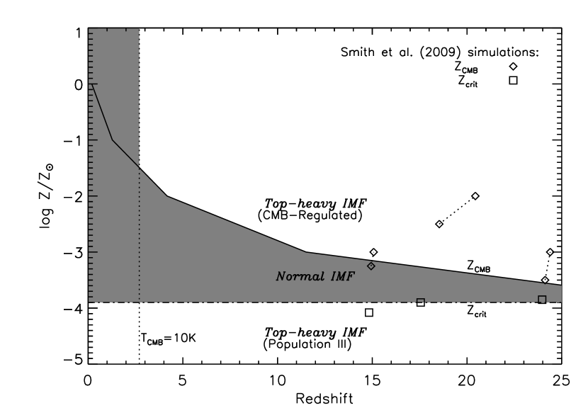
Figure 1.— Estimated evolution of $Z_{\mathrm{CMB}}$ as a function of redshift (solid line), above which fragmentation is inhibited due to the CMB. The dot-dashed line shows the critical metallicity $Z_{\mathrm{crit}}$, below which fragmentation is inhibited due to inefficient cooling; we use the value $\log Z/Z_{\sun}=-3.9$, from the Set 2 simulations of Smith et al. (2009). The region in between these lines, where a normal IMF is expected, is shaded. The dotted vertical line at $z=2.7$ denotes when the CMB temperature drops below $10$ K; the CMB is not expected to be important below this point. The results of Smith et al. (2009) are also shown; the squares denote the values of $Z_{\mathrm{crit}}$ they calculated for each of their sets of initial conditions, while the pairs of connected diamonds denote the range of possible values of $Z_{\mathrm{CMB}}$. Note that because the same initial conditions collapsed at different redshifts for different metallicities, the pairs of diamonds are not vertical.

The best estimates of $Z_{\mathrm{CMB}}$ to date come from Smith et al. (2009), who performed ab initio simulations with three different sets of initial conditions and a variety of metallicities. The amount of fragmentation they found in the simulations depended on metallicity: at low metallicities, no fragmentation was seen because the gas remained hot; at intermediate metallicities, the gas fragmented; and at high metallicities, there was again no fragmentation because the gas cooled so quickly that it reached the CMB temperature. Because simulations can only be performed for a discrete set of metallicities, we cannot determine the exact value of $Z_{\mathrm{CMB}}$ in each case, but we can bound it on the lower end by the most metal-rich simulation where fragmentation occured, and on the upper end up the least metal-rich simulation where fragmentation did not occur. These are plotted in Figure 1 as the connected diamonds, at the redshifts at which each simulation collapsed. Note that although the Set 2 simulations collapse at a redshift intermediate between the Set 1 and Set 3 simulations, their implied $Z_{\mathrm{CMB}}$ is higher, demonstrating that the boundary between the normal and CMB-regulated regimes is not purely a function of metallicity, but also depends on the details of the initial conditions; Jappsen et al. (2009) make a similar point regarding the lower metallicity threshold, $Z_{\mathrm{crit}}$.

It is difficult to determine the consequences of CMB regulation purely from these simulations because very little star formation occurs at such high redshifts. We must therefore devise a method of estimating the evolution of $Z_{\mathrm{CMB}}$ as a function of redshift. To do this, we note that in the numerical models of Omukai et al. (2005) and Smith et al. (2009), the CMB effectively acts as a temperature floor to the cooling collapsing protostellar core. Without the CMB, the normal evolution of the core is to cool and collapse until heat is released by rapid $\mathrm{H_{2}}$ formation via three-body collisions, which drives a rise in temperature. Once all of the hydrogen is in molecular form, cooling once again dominates and the temperature drops. Eventually the core becomes optically thick, at which point the dust emission can no longer cool the core, and the temperature rises again due to compressional heating. There is a minimum temperature ${T_{\mathrm{min}}}(Z)$ that the gas reaches during this evolution (either immediately before the onset of the three-body reaction or immediately before the core becomes optically thick), which depends on its cooling history and therefore its metallicity. Our ansatz is as follows: at redshift $z$, the CMB regulates star formation in gas of metallicity $Z$ if the CMB temperature

$${T_{\mathrm{CMB}}}(z)>{T_{\mathrm{min}}}(Z),$$ (1)

where the CMB temperature at redshift $z$ is

$${T_{\mathrm{CMB}}}(z)=T_{0}(1+z),$$ (2)

for present-day CMB temperature $T_{0}=2.726$ K. If the effect of the CMB is to act as a temperature floor, this condition defines the regime where the CMB can have an effect. We determine ${T_{\mathrm{min}}}(Z)$ from the tracks of Omukai et al. (2005), who modelled the evolution of temperature and density for a series of metallicities $Z/Z_{\sun}=0$, $10^{-6}$, $10^{-5}$, $10^{-4}$, $10^{-3}$, $10^{-2}$, $10^{-1}$, $10^{0}$. For each of these metallicities, we can then determine the redshift where equation (1) is satisfied.

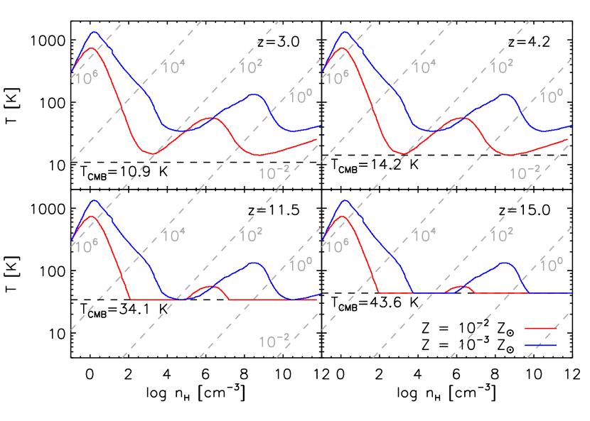
Figure 2.— Density-temperature evolution of a protostellar core with metallicity $Z=10^{-2}~{}Z_{\sun}$ ($10^{-3}~{}Z_{\sun}$) in red (blue) from Omukai et al. (2005), with a temperature floor set by the CMB temperature at each of the four labelled redshifts. The horizontal dashed lines denote the CMB temperature at each redshift. For $Z=10^{-2}~{}Z_{\sun}$, ${T_{\mathrm{min}}}=14.2$ K, while for $Z=10^{-3}~{}Z_{\sun}$, ${T_{\mathrm{min}}}=34.1$ K. The diagonal dashed gray lines indicate lines of constant Jeans mass, and are labelled in $M_{\sun}$.

This is demonstrated in Figure 2, where we have plotted the density-temperature evolution of protostellar cores of two different metallicities ($\log Z/Z_{\sun}=-2$, $-3$) from Omukai et al. (2005). In each of the four panels, we have imposed a temperature floor given by $T_{\mathrm{CMB}}$ at a different redshift. At $z=3$, ${T_{\mathrm{CMB}}}=10.9$ K, which is colder than either core ever reaches, and the CMB has no effect. At $z=4.2$, ${T_{\mathrm{CMB}}}=14.2$ K, which is the exact minimum temperature that the $\log Z/Z_{\sun}=-2$ protostar reaches; if the CMB temperature were any higher, it would affect the core evolution. This can be seen at $z=11.5$, when ${T_{\mathrm{CMB}}}=34.1$ K; the $\log Z/Z_{\sun}=-2$ core does not cool nearly as far, and the CMB temperature just reaches the minimum temperature of the $\log Z/Z_{\sun}=-3$ protostar. At $z=15$, the temperature floor imposed by the CMB clearly affects the evolution of both cores. We therefore adopt ${Z_{\mathrm{CMB}}}(z=4.2)=10^{-2}~{}Z_{\sun}$ and ${Z_{\mathrm{CMB}}}(z=11.5)=10^{-3}~{}Z_{\sun}$. We perform the same calculation for each metallicity track in Omukai et al. (2005) and plot the relationship as the solid line in Figure 1.

Fragmentation is only expected to be efficient when the Jeans mass rapidly decreases, i.e. when the tracks move downward. Therefore the characteristic mass scale is the Jeans mass when the core stops cooling (Larson, 2005). Lines of constant Jeans mass are shown as the diagonal dashed gray lines in Figure 2. For the $Z=10^{-2}~{}Z_{\sun}$ track, this characteristic scale is $0.2~{}M_{\sun}$, but at redshift $z=11.5$ it rises to $50~{}M_{\sun}$. The top-heavy IMF is a direct consequence of this dramatic change in the characteristic mass scale at the end of fragmentation.

Because the temperature of the protostellar core only just reaches the CMB temperature, it is unlikely that the CMB has much effect at the exact redshift we calculate. The ${T_{\mathrm{CMB}}}(z)$, and therefore $z$, that we calculate for each metallicity must be a slight underestimate, or correspondingly the $Z_{\mathrm{CMB}}$ that we calculate at each redshift must be a slight underestimate.

Our estimated $Z_{\mathrm{CMB}}$ matches the simulation results of Smith et al. (2009) very well for their Set 1 initial conditions, mildly underpredicts it for their Set 3 intial conditions, and underpredicts it by about an order of magnitude for their Set 2 initial conditions. We should therefore expect that the transition between a normal and top-heavy IMF occurs at metallicities somewhere between our predicted $Z_{\mathrm{CMB}}$ and a metallicity ten times larger, with the details depending on the properties and formation history of the individual halos in which the star formation occurs.

Although our estimate for $Z_{\mathrm{CMB}}$ is well-defined down to $z\approx 0.2$, it is unlikely that CMB regulation is truly important at these redshifts. As noted by Smith et al. (2009), gas clouds in the local ISM are not observed to cool below $10$ K; therefore, when the CMB drops below this temperature, it can no longer affect the thermal evolution of protostellar gas. This occurs at $z=2.7$, denoted by the vertical dotted line in Figure 1.

As discussed earlier, a top-heavy IMF is also expected for Population III stars, with metallicities below $Z_{\mathrm{crit}}$, denoted by the horizontal dot-dashed line in Figure 1. A normal IMF is therefore expected in the shaded region of Figure 1; at lower metallicities, cooling is too inefficient for fragmentation to occur, while at higher metallicities, the gas cools immediately to the CMB temperature where it becomes isothermal and does not fragment. Although the estimates of the boundaries of the region are rough, they provide a guideline for the star formation events that would have been influenced by the CMB.

It is interesting that our derived $Z_{\mathrm{CMB}}$ rises substantially from $<10^{-3}~{}Z_{\sun}$ at $z>10$ to $\sim 10^{-1.5}$ at $z\sim 3$. Such metallicities are typical for old stellar populations, and it is therefore plausible that CMB regulation could have been important for stars formed at these redshifts.

3. Cosmic Metallicity Evolution

In order to determine the effects of CMB-regulated star formation, we must estimate, at each redshift $z$, the fraction of stars that formed with metallicities $Z>{Z_{\mathrm{CMB}}}(z)$. Observational measurements are available at $z\lesssim 3$ from stellar population modelling of the integrated spectra of galaxies from the Sloan Digital Sky Survey (SDSS; Panter et al., 2008), but, as discussed in § 2, the effects of the CMB are only likely to be significant at $z\gtrsim 3$. We must therefore use theoretical models to estimate the cosmic evolution of the metallicity of star-forming gas.

3.1. Simulations

Our simulations were performed as part of the McMaster Unbiased Galaxy Simulations project (MUGS), a campaign to construct high resolution simulations of a large set of $L^{*}$ galaxies that randomly sample the sites of galaxy formation, including a full range of modern galaxy formation physics. Full details of the MUGS simulations will be presented in Stinson et al. (in preparation); we provide an overview of the most important properties of the simulations below.

The simulations were performed using a WMAP 3 $\Lambda$CDM cosmology with $H_{0}=73~{}\mathrm{km~{}s^{-1}~{}Mpc^{-1}}$, $\Omega_{m}=0.24$, $\Omega_{\Lambda}=0.76$, $\Omega_{\mathrm{bary}}=0.04$, and $\sigma_{8}=0.76$ (Spergel et al., 2007). Halos were chosen from a uniform-resolution $256^{3}$ dark matter-only simulation in a box of side $50~{}h^{-1}$ Mpc using the friends-of-friends algorithm (Davis et al., 1985). A random selection of isolated halos with masses $4\times 10^{11}~{}M_{\sun}\leq M\leq 2\times 10^{12}~{}M_{\sun}$ were chosen for resimulation at higher resolution with full baryonic physics. The highest resolution dark matter region, encompassing all matter out to $5~{}r_{\mathrm{vir}}$, has particle mass $m_{\mathrm{DM}}=1.1065\times 10^{6}~{}M_{\sun}$, while gas particles are placed inside $3~{}r_{\mathrm{vir}}$ and have initial masses $m_{\mathrm{gas}}=2.2131\times 10^{5}~{}M_{\sun}$. There are typically $\sim 1000000$ gas and high resolution dark matter particles each in the refined regions of the resimulations, with the exact number depending on the halo mass and the geometry of the Lagrangian region that collapses into the $z=0$ halo.

The simulations were evolved using the parallel SPH code gasoline (Wadsley et al., 2004). gasoline solves the equations of hydrodynamics using SPH and self-gravity using the Barnes-Hut tree algorithm (Barnes & Hut, 1986), and includes radiative cooling, an ultraviolet (UV) background, star formation, and energetic and chemical feedback.

The cooling is calculated from the contributions of both primordial gas and metals as $\Lambda_{\mathrm{tot}}(z,\rho,T,Z)=\Lambda_{\mathrm{HI,HeI,HeII}}(z,\rho,T)+\frac{Z}{Z_{\sun}}\Lambda_{\mathrm{metal},Z_{\sun}}(z,\rho,T)$. The first term employs atomic cooling based on a gas with primordial composition heated by a uniform UV ionizing background, adopted from Haardt & Madau (in preparation; see Haardt & Madau, 2001) with rates coefficient closely matching those cited in Abel et al. (1997), while the metal cooling grid is constructed using Cloudy (version 07.02, last described by Ferland et al. (1998)), assuming ionization equilibrium, as described in Shen et al. (2009). The UV background is used in order to calculate the metal cooling rates self-consistently. The cooling lookup table is linearly interpolated in three dimensions (i.e., $\rho$, $z$, $T$) and scaled linearly with metallicity.

The star formation and feedback recipes are based on the “blastwave model” described in detail in Stinson et al. (2006), but with the addition of clustered supernovae to account for the clustered nature of star formation. Star formation can occur in gas particles that are dense ($n_{\rm min}=0.1~{}\mathrm{cm^{-3}}$) and cool ($T_{\rm max}=15,000$ K), calibrated to match the Kennicutt (1998) Schmidt Law for the Isolated Model Milky Way in Stinson et al. (2006).

At the resolution of these simulations, each star particle represents a large number of stars ($6.32\times 10^{4}~{}M_{\sun}$). Thus, each particle has its stars partitioned into mass bins based on the initial mass function presented in Kroupa et al. (1993). These masses are correlated to stellar lifetimes as described in Raiteri et al. (1996). We stochastically determine when a star particle releases feedback energy so that a minimum of $30$ supernovae worth of energy is released concurrently to reflect the clustered nature of star formation. The explosion of these stars is treated using the analytic model for blastwaves presented in McKee & Ostriker (1977) as described in detail in Stinson et al. (2006). While the blast radius is calculated using the full energy output of the supernova, less than half of that energy is transferred to the surrounding ISM, $E_{SN}=4\times 10^{50}$ ergs. The rest of the supernova energy is radiated away. Iron and oxygen are produced in SNII according to the analytic fits used in Raiteri et al. (1996). The iron and oxygen are distributed to the same gas within the blast radius as is the supernova energy ejected from SNII. Each SNIa produces $0.63~{}M_{\sun}$ iron and $0.13~{}M_{\sun}$ oxygen (Thielemann et al., 1986) and it is ejected into the nearest gas particle for SNIa.

We have implemented diffusion of all scalar SPH quantities, particularly metal content and thermal energy, as described in Shen et al. (2009), which is required to correctly model even simple processes such as convection and Rayleigh-Taylor instabilities (Wadsley et al., 2008) and to account for mixing in turbulent outflows.

MUGS galaxies are labelled by their group number in the list returned by the friends-of-friends algorithm. The simulations analyzed in this work are MUGS g$1536$, g$5664$, g$7124$, g$15784$, g$21647$, g$22437$, g$22795$, and g$24334$. Only stars within the virial radius of the main galaxy are considered.

3.2. Metallicity Evolution

Figure 3.— Metallicity of stars as a function of their formation redshift. The solid line is the mean from the MUGS simulations, the dotted line is the mean from the simulation of Davé & Oppenheimer (2007), and the dot-dashed line is the observed mean metallicity of star-forming gas at each redshift, as determined from spectral synthesis modelling of SDSS galaxies (Panter et al., 2008).

The mean metallicity of stars formed in the simulation is shown in Figure 3 as a function of their formation redshift. The solid line shows the results for all stars within MUGS simulated galaxies, and shows that stellar metallicities rise from $\sim-3$, for those formed at $z\gtrsim 10$, to nearly solar for those formed at $z=0$. Our simulations are of $L^{*}$ galaxies, while the majority of star formation at high redshift occurred in larger galaxies, which formed their metals earlier than less massive galaxies. Our determinations may therefore underestimate the metallicities of a universal sample of stars formed at high redshift.

We have confirmed that our results are consistent with those obtained with completely different codes: the dotted line, which shows the star-formation-rate-weighted mean metallicity of gas from the GADGET2 simulations of Davé & Oppenheimer (2007) (the “SFR-weighted” line in their figure 2) and should be directly comparable, shows reasonable agreement with our results over the entire range $0\leq z\leq 6$ that they plotted. Where our results deviate from those of Davé & Oppenheimer (2007), it is in the sense that the MUGS metallicities are lower.

The best observational measurements of stellar metallicity as a function of formation redshift come from Panter et al. (2008), who performed spectral synthesis modelling of SDSS galaxies at redshifts ranging from $0.1$ to $3$. The mean metallicities of stars inferred to have formed at each redshift is shown as the dot-dashed line in Figure 3. Unlike the simulation predictions, the observations show essentially no drop in stellar metallicity out to $z=3$. This is mainly because the total stellar mass is dominated by the most massive galaxies, which formed most of their stars very early; however, the stellar metallicities within galaxies of stellar mass $3\times 10^{10}~{}M_{\sun}\leq M_{*}\leq 1\times 10^{11}~{}M_{\sun}$ show almost identical behavior, and this is very nearly the same mass range as the MUGS galaxies ($4\times 10^{10}~{}M_{\sun}<M_{*}<1.2\times 10^{11}~{}M_{\sun}$), and the mass range that includes the Milky Way ($M_{*}\approx 5\times 10^{10}~{}M_{\sun}$; Klypin et al., 2002; Widrow et al., 2008). We may therefore conclude that our simulations do not overpredict the metallicity of star-forming gas at high redshifts, and may even underpredict it, an issue we will return to in § 4.5.

4. Consequences of CMB regulation

4.1. When was the CMB important?

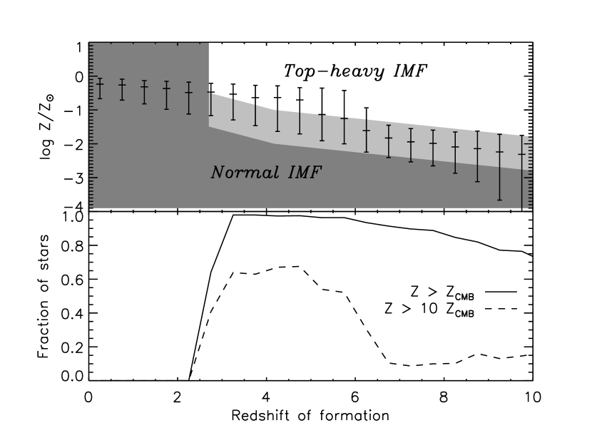
Figure 4.— (Top) The data points denote the median metallicity of stars formed at each redshift within the MUGS simulations, while the error bars denote the 10th and 90th percentiles. Stars formed within the dark shaded region, which is identical to the shaded region in Figure 1, are expected to form with a normal IMF. The light shaded region extends to metallicities $1$ dex higher than $Z_{\mathrm{CMB}}$, where stars may form with either a normal or top-heavy IMF, if CMB regulation occurs. All stars formed in the white region are expected to exhibit a top-heavy IMF if the CMB regulation hypothesis is correct. (Bottom) Fraction of stars formed with metallicities greater than $Z_{\mathrm{CMB}}$, i.e. within the light shaded or white regions of the top panel. The dashed line denotes the fraction of stars formed with metallicities greater than $10~{}{Z_{\mathrm{CMB}}}$, i.e. within the white region of the top panel.

We have plotted our estimate of the metallicity of star-forming gas from § 3 over our estimate of the critical metallicity for CMB regulation, $Z_{\mathrm{CMB}}$, from § 2, in the top panel of Figure 4. Note that unlike in Figure 3, here we plot the median metallicity, along with the 10th and 90th percentiles.

The first remarkable thing to note about Figure 4 is that the median star was formed with $Z>{Z_{\mathrm{CMB}}}$ at almost all redshifts greater than $2.7$. In other words, if the CMB regulation hypothesis is correct, the majority of stars at high redshift were formed in the CMB-regulated regime. While this statement is subject to uncertainties in both our estimate of $Z_{\mathrm{CMB}}$ and in the cosmic metallicity evolution measured from the simulations, it would appear that the CMB influenced a significant amount of star formation at high redshift.

In the bottom panel of Figure 4, we have plotted the fraction of stars that form at $Z>{Z_{\mathrm{CMB}}}$ in the simulation. As expected from the top panel, this is very high: over $80\%$ at virtually all redshifts where the CMB temperature is higher than $10$ K. Given the uncertainties in both the estimate of $Z_{\mathrm{CMB}}$ and in the metallicity evolution predictions of the simulation, we have also determined the fraction of stars formed with metallicity $Z>10~{}{Z_{\mathrm{CMB}}}$ (dashed line). We consider it unlikely that the combined difference between the simulation metallicities and the $Z_{\mathrm{CMB}}$ estimate is a full order of magnitude; moreover, Figure 3 strongly suggests that the simulated metallicities are more likely underestimates than overestimates, which would imply that an even larger fraction of stars formed with $Z>{Z_{\mathrm{CMB}}}$ or $Z>10~{}{Z_{\mathrm{CMB}}}$ than has been calculated. However, even with this drastic change, half of the stars formed at $2.7<z<6$ are formed in the CMB-regulated regime, a fraction that drops to $10$–$15\%$ at higher redshift.

Our first major conclusion is therefore that if the CMB regulation hypothesis is correct, the CMB must have influenced the majority of star formation at $3\lesssim z\lesssim 6$, and may have been important to even higher redshift.

4.2. Supernova and Gamma Ray Burst Rates

Stars whose initial masses are at least $M_{\mathrm{SN}}\sim 8~{}M_{\sun}$ end their lives as core-collapse supernovae. The fraction of stars above this limit, and therefore the number of supernovae produced per unit mass of stars depends on the IMF: a top-heavy IMF produces more supernovae. For a truncated power-law IMF, this ratio is given by

$$\frac{N_{\mathrm{SN}}}{M_{*}}=\frac{(\alpha+2)(M_{\mathrm{max}}{}^{\alpha+1}-M_{\mathrm{SN}}{}^{\alpha+1})}{(\alpha+1)(M_{\mathrm{max}}{}^{\alpha+2}-M_{\mathrm{min}}{}^{\alpha+2})}$$ (3)

(Bailin & Harris, 2009). The IMF may be top-heavy in the sense of having a flatter slope $\alpha$, or be “bottom-light” in the sense of having a higher minimum stellar mass $M_{\mathrm{min}}$. To give an example of the quantitative size of the effect, flattening the slope from the canonical Salpeter value of $\alpha=-2.35$ to $\alpha=-2.1$ increases the supernova rate by $50\%$, while increasing $M_{\mathrm{min}}$ from $0.30~{}M_{\sun}$ to $5~{}M_{\sun}$ increases the supernova rate by a factor of $3.5$. If the CMB-regulation hypothesis is correct, and the majority of star formation at $3\lesssim z\lesssim 6$ occurred with a top-heavy IMF, then predictions of the high-redshift supernova rate (e.g. Dahlén & Fransson, 1999) are underestimates by a corresponding factor. Some indirect consequences of this are discussed in sections 4.3 and 4.5.

The link between core-collapse supernovae and long duration gamma ray bursts (GRBs) is now well established (Woosley & Bloom, 2006). One might therefore expect that a top-heavy IMF, which increases the supernova rate, might also increase the GRB production rate. However, there is both observational and theoretical evidence that GRBs are preferentially produced by metal-poor stars (e.g. Yoon et al., 2006; Wolf & Podsiadlowski, 2007). As CMB regulation results in a top-heavy IMF only at high metallicities, it is not obvious whether it would result in an enhancement of the GRB rate without more detailed modelling.

4.3. Reconstructing the cosmic star formation history

A key goal in the study of galaxy formation is to reconstruct the cosmic star formation history (e.g. Lilly et al., 1996; Madau et al., 1996). There are three types of methods for performing this measurement: the first is to directly measure indicators of current star formation (such as H$\alpha$, UV, far-infrared, or radio continuum emission) in galaxies at a variety of redshifts; the second is to deconstruct the stellar populations of low-redshift galaxies to determine their ages; and the third is to examine the stellar mass density in galaxies at a variety of redshifts, which is the integral of the star formation rate minus the stellar death rate over time. The first of these methods is direct: it measures star formation as it happens, while the latter two methods are indirect and rely on the stars that are produced.

A key assumption in the indirect methods is the IMF: the mass of stars remaining after a given length of time from a fixed burst of star formation depends strongly on their mass distribution. If the IMF is very top-heavy, then the number of extant stars a given length of time later will be smaller than if the IMF is normal. In the extreme case where all stars are massive, then a burst of star formation will leave no visible stellar population a short time after the burst, and will be completely missed by any method that relies on the stars to measure the rate of star formation.

Some of the direct star formation rate indicators also depend on the IMF. For example, most radio continuum emission in star-forming galaxies is synchrotron radiation from relativistic electrons that are accelerated in supernova remnants (Condon, 1992). As discussed in § 4.2, a top-heavy IMF increases the supernova rate with respect to the star formation rate, and therefore must also increase the radio continuum emission. Therefore, a top-heavy IMF both increases the derived star formation rate from direct indicators, and decreases the derived rate from indirect indicators.

In fact, these measurement methods do not agree. At high redshift, the direct measurements of the star formation rate are systematically higher than the indirect methods. This can be seen in Heavens et al. (2004), who perform spectral synthesis modelling of SDSS galaxies at low redshift to determine their stellar populations, and use them to infer the star formation rate at redshifts up to $10$. They find that their star formation rates are systematically lower than the direct measurements in their higher redshift bins, precisely where CMB regulation would be expected to be important.

A similar result comes from Wilkins et al. (2008), who used measurements of the stellar mass density as a function of redshift. The time derivative of this is the net change in stellar mass, which is the rate of star formation minus the rate that stars die. The latter term is a strong function of the IMF, and is much higher for a top-heavy IMF, requiring a much larger star formation rate to fit the same data. These authors find that their implied star formation history is consistent with direct measurements out to $z=0.7$, but becomes increasingly discrepant at higher redshift, reaching a factor of $4$ by $z=3$. They suggest that an increasingly top-heavy IMF could explain this discrepancy, but do not offer a physical mechanism for this evolution. Although CMB regulation offers a natural explanation for why the IMF would change with time, one problem is that Wilkins et al. (2008) find evidence for a discrepancy between the direct and indirect star formation rates down to redshifts of $z=0.7$, while CMB regulation is unlikely to operate much below $z=2.7$. However, the discrepancy is relatively mild between $z=0.7$ and $z=2$, and it is only beyond $z=2$ that the differences become significant.

Similar considerations drove Davé (2008) to suggest an average IMF that slowly evolves with time; although he mentions the influence of the CMB as a potential driver for this evolution, the model is expressed as an overall gradual change with redshift rather than a change that specifically operates in the high-metallicity high-redshift regime. Fardal et al. (2007) perform a similar exercise while also considering the energy contained in the extragalactic background light (which is dominated by light from stars formed at $z<2.6$) as a constraint, and find that the best way to reconcile the measurements is with a top-heavy IMF, which they suggest occurs in the starbursting galaxies that are increasingly common at redshifts beyond where the extragalactic background is generated. A CMB-regulated top-heavy IMF would perform a very similar function.

4.4. Globular Cluster Bimodality

A conundrum in the study of globular cluster systems around galaxies is the observed bimodality of their metallicity distribution (e.g. Harris et al., 2006). A possible explanation is that metal-poor clusters formed during the initial collapse of the protogalaxy, while the metal-rich population formed during subsequent major mergers. However, the metal-poor peak covers a narrow range in metallicity, which appears to be impossible to reproduce unless the formation of metal-poor clusters was abruptly truncated (Beasley et al., 2002).

However, if CMB-regulated star formation results in mostly or exclusively massive stars, there is another possibility: the first round of globular cluster formation did occur over a wide range of metallicities from $\log Z/Z_{\sun}\sim-2.5$ upward, but the ones with $\log Z/Z_{\sun}\gtrsim-1$ would have formed with a top-heavy IMF. The massive stars in the cluster would have died quickly, shedding the majority of their mass in the form of stellar winds and supernova ejecta. If the massive stars made up a significant fraction of the cluster mass, as they would if the IMF were sufficiently top-heavy, this dramatic loss of binding mass would result in the gravitational unbinding and dispersion of the cluster.

In other words, the sharpness of the low-metallicity peak and the relative absence of intermediate-metallicity clusters near $\log Z/Z_{\sun}\sim-1$ may be entirely an artifact of a top-heavy IMF: higher metallicity clusters formed along with their lower-metallicity brethren, but did not survive to the present day.

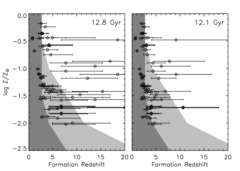
Figure 5.— Metallicity versus formation age of Milky Way globular clusters. Data come from Marín-Franch et al. (2009). The relative ages have been converted into formation redshift by assuming (1) the WMAP 5 recommended cosmological parameter values (Hinshaw et al., 2009), and (2) an absolute age scale of $12.8$ Gyr and $12.1$ Gyr for the left and right panels respectively. The dark shaded region is the region expected to exhibit a normal IMF, and is identical to the shaded region in Figure 1. The light shaded region also includes metallicities up to $1$ dex larger, as in Figure 4.

In the left panel of Figure 5, we have repeated the shaded and light shaded regions from Figure 4 that denote the range in redshift and metallicity where a normal IMF would be expected, while the unshaded regions are those where CMB regulation, if it occurs, would result in a top-heavy IMF. We have overplotted the formation redshifts and metallicities of Milky Way globular clusters from the main sequence fitting performed by Marín-Franch et al. (2009). We have used the ages based on the Dotter et al. (2007) isochrones, and assumed that a normalized age of $1$ corresponds to an absolute age of $12.8$ Gyr, consistent with the Dotter et al. (2007) models. These absolute ages have been converted to formation redshift by assuming the WMAP 5 recommended cosmological parameter values including the results of WMAP, baryon accoustic oscillations, and type Ia supernovae (the WMAP+BAO+SN set of Hinshaw et al., 2009). While the relative ages are precise to within $2\%$–$7\%$, at high redshift a very small variation in age corresponds to a large variation in redshift, and so the horizontal error bars in Figure 5 are very large at high redshift. We have assumed the Zinn & West (1984) metallicity scale.

Examination of the left-hand panel of Figure 5 reveals that there are many GCs that have metallicities significantly larger than the $Z_{\mathrm{CMB}}$ at which they formed, i.e. above the dark shaded region, even given the large uncertainties in the formation redshifts due to the finite precision of the relative ages. However, if we assume that normal star formation can occur at metallicities up to $1$ dex higher than $Z_{\mathrm{CMB}}$, i.e. in both the dark and light shaded regions, then the vast majority of GCs lie within the permitted region and only a few spill over into the forbidden region; the most discrepant clusters are Lyngå 7, NGC 6171, NGC 6717, and NGC 6362. Are the existence of these clusters then conclusive evidence that CMB regulation is not important?

It is interesting that three of these four clusters, NGC 6171, NGC 6362, and NGC 6717, lie in the less populated $\log Z/Z_{\sun}\sim-1$ metallicity regime between the metal-poor and metal-rich peaks, and that all of these clusters are quite low mass. Perhaps these objects are incompletely-disrupted remnants of a larger population of clusters that once inhabited the same parameter space, or perhaps the transition from a normal IMF to a strongly top-heavy IMF is gradual and these clusters formed with only a slightly top-heavy IMF. In these cases, we might expect to see systematic differences between the stellar mass functions of these clusters compared to those of other Galactic GCs; detailed luminosity functions of these clusters would be well worth measuring to assess the viability of this explanation.

However, we caution against overinterpretation of the location of these clusters. A serious concern is the ages: while the relative ages of clusters are precise, there is still large systematic uncertainty in the absolute age scale. The effects of this can be seen clearly by comparing the left-hand panel of Figure 5 to the right-hand panel, where we have reduced the absolute age scaling by $5\%$ to $12.1$ Gyr. With this small change, the majority of GCs are consistent with forming at metallicities below $Z_{\mathrm{CMB}}$, and the only cluster that is clearly in the forbidden region is Lyngå 7. The age of this particular cluster is suspect, however; other determinations of its age make it much younger (Ortolani et al., 1993; Sarajedini, 2004), and its location in the bulge introduces large uncertainties due to significant reddening.

Because of the large inherent formation redshift uncertainties, we are not able to come to any firm conclusions regarding whether CMB-regulated star formation has shaped the population of extant globular clusters, although they appear to be consistent with the CMB-regulation hypothesis if the few discrepant clusters are indeed remnants of a disrupted population or simply observational spill over. Perhaps if more precise absolute ages of GCs can be determined in the future, or if the detailed luminosity functions of the interesting clusters can be measured, it may be possible to address this issue more conclusively.

4.5. Abundances and Abundance Patterns

A top-heavy IMF in metal-rich high-metallicity star formation may leave characteristic patterns in the evolution of both the global metallicity and the abundances of particular elements. Not only does a top-heavy IMF increase the number of supernovae produced, but it also increases the average mass of the supernova progenitors. More massive stars eject a larger fraction of their mass in the form of newly-synthesized metals, and are particularly efficient at forming $\alpha$ elements such as oxygen, neon and magnesium (e.g. Woosley & Weaver, 1995).

In fact, there is a slight inconsistency in using our simulations, which assume a normal IMF, to predict the fraction of star formation that occurs with a top-heavy IMF, as in § 3. If a large fraction of high-redshift star formation occurred in the CMB-regulated regime, as we predict, then they must have ejected a larger mass of metals into their environment, and therefore the global metallicity of the universe must have risen more steeply when CMB regulation was important, between at least $z=6$ and $z=3$, than the simulations predict. This would result in an even larger fraction of high-redshift star formation occuring in the CMB-regulated regime; however, we already predict that the majority of high-redshift star formation occured above $Z_{\mathrm{CMB}}$, so this inconsistency does not qualitatively affect our conclusions.

However, this more rapid rise in the global metallicity is precisely what is required to reconcile the discrepancy between the metallicities predicted by the simulations, $\log Z/Z_{\sun}\sim-0.5$ at $z=3$, and those observed, which reach solar metallicity by the same redshift (see Figure 3).

A top-heavy IMF may also leave an imprint on the abundance patterns. Core collapse supernovae from high mass progenitors eject a larger fraction of their mass in the form of $\alpha$-elements, especially $\mathrm{{}^{16}O}$, but also $\mathrm{{}^{20}Ne}$, and $\mathrm{{}^{24}Mg}$ (Woosley & Weaver, 1995; Nomoto et al., 1997). Therefore, a top-heavy IMF may produce more $\alpha$ elements than a population with a normal IMF.

Current Galactic chemical evolution models accurately reproduce the observed abundance patterns of Galactic stars over a large range of metallicities, leaving little room for significant changes. However, one element whose abundances are not well reproduced is Mg, which is systematically underpredicted by the models over the range $-2.5\lesssim{[\mathrm{Fe}/\mathrm{H}]}\lesssim-0.5$ (and slightly overpredicted at lower metallicities; see figure 1 of François et al., 2004). Interestingly, these are precisely the metallicities where most of the CMB-regulated star formation occurs within our simulations, and $\mathrm{{}^{24}Mg}$ would indeed be produced at greater rates with a top-heavy IMF. However, the O abundances do not support this conjecture: they are, if anything overpredicted at these metallicities, while a top-heavy IMF would have an even larger effect on $\mathrm{{}^{16}O}$ than on $\mathrm{{}^{24}Mg}$. Unless some unaccounted-for process systematically drives down the $\mathrm{{}^{16}O}$ abundance by a significant amount, a more parsimonious explanation is that the yields require adjustment, as suggested by François et al. (2004).

5. Conclusions

We have investigated the suggestion of Larson (2005) and Smith et al. (2009) that star formation at high redshift and high metallicity results in a top-heavy IMF due to the influence of the CMB as an effective temperature floor for the collapsing protostellar core. By assuming that CMB regulation is important if the minimum temperature the core would reach in the absence of the CMB, according to the models of Omukai et al. (2005), is less than the CMB temperature at a given redshift, we are able to parametrize the evolution of the critical metallicity $Z_{\mathrm{CMB}}$ as a function of redshift. Comparison with the 3D hydrodynamical simulations of Smith et al. (2009) suggests that our model is generally accurate, but may underestimate $Z_{\mathrm{CMB}}$ by up to an order of magnitude in particular cases.

By comparing $Z_{\mathrm{CMB}}$ to the metallicities of stars formed in high resolution cosmological simulations of the formation of eight $\sim L_{*}$ galaxies, we conclude that if CMB regulation does operate, the majority of stars at redshifts between $2.7$ and $6$ would have formed in the CMB-regulated regime. We have investigated five possible observational signatures of CMB regulation:

1. Current predictions of supernova rates, and possibly GRB rates, are underestimates at $z\gtrsim 3$.

2. Indirect measures of the star formation history based on the stellar populations left behind by episodes of star formation, such as the age distribution of local stellar populations and evolution of the stellar mass density as a function of redshift, would systematically underestimate the star formation rate at redshifts greater than $2.7$ compared to measurements based on UV and far-infrared flux generated directly by star formation. Such a discrepancy is seen, although it appears to extend to lower redshift.

3. Globular clusters that formed at high metallicity and high redshift may have quickly evaporated, leaving no present-day evidence of their existence, possibly explaining the relatively narrow metallicity range of the metal-poor GC population. In this case, we would expect there to be no extant GCs that are both metal-rich and formed at very high redshift. Because of the difficulties in determining absolute ages to old GCs, and the steepness of the age-redshift relation at high redshift, current data are not able to constrain this hypothesis.

4. Cosmic metallicity may rise more rapidly at early times than predicted by current simulations that assume a normal IMF, reaching solar metallicities at higher redshift. This could reconcile the simulations with observations that show a mean metallicity of approximately solar for stars formed out to redshift $3$.

5. Elements produced by high-mass supernova progenitors, particularly the $\alpha$ elements O, Ne, and Mg, would be produced with greater abundance between redshifts $6$ and $3$, or ${[\mathrm{Fe}/\mathrm{H}]}\sim-2$ to $-0.5$, than predicted in models that assume a normal IMF. This could help explain the high Mg abundances seen in stars of this metallicity range in the Galaxy, but would exacerbate the overprediction of O over the same range in metallicities. Since the O yields are more sensitive to the IMF, we conclude that the abundance patterns are not produced by a top-heavy IMF, although a bottom-light IMF would not alter the abundances.

In conclusion, the observations neither provide conclusive evidence for the hypothesis that the CMB can regulate star formation, nor rule it out. The most convincing evidence would come in the form of either the clear presence or absence of an envelope in redshift-metallicity space, above which stars are either absent or have greatly reduced numbers compared to the number of stars believed to have formed there from other measurements; unfortunately, as discussed in § 4.4, it is unclear if stellar ages will ever be known precisely enough to perform this test. Another potential avenue of exploration would be to use the methods that currently argue for a mean change in the IMF with time, such as in Davé (2008) and Wilkins et al. (2008), but subdividing the populations by metallicity to determine if an evolving IMF is only required for metal-rich stars, as would be expected if the evolution in the IMF is due to CMB regulation, or if it must be truly universal.

References

- Abel et al. (1997) Abel, T., Anninos, P., Zhang, Y., & Norman, M. L. 1997, New Astronomy, 2, 181
- Abel et al. (2002) Abel, T., Bryan, G. L., & Norman, M. L. 2002, Science, 295, 93
- Alves et al. (2007) Alves, J., Lombardi, M., & Lada, C. J. 2007, A&A, 462, L17
- Bailin & Harris (2009) Bailin, J., & Harris, W. E. 2009, ApJ, 695, 1082
- Barnes & Hut (1986) Barnes, J., & Hut, P. 1986, Nature, 324, 446
- Beasley et al. (2002) Beasley, M. A., Baugh, C. M., Forbes, D. A., Sharples, R. M., & Frenk, C. S. 2002, MNRAS, 333, 383
- Bromm et al. (2001) Bromm, V., Ferrara, A., Coppi, P. S., & Larson, R. B. 2001, MNRAS, 328, 969
- Chabrier (2003) Chabrier, G. 2003, in IAU Symposium, Vol. 221, IAU Symposium, 67
- Condon (1992) Condon, J. J. 1992, ARA&A, 30, 575
- Dahlén & Fransson (1999) Dahlén, T., & Fransson, C. 1999, A&A, 350, 349
- Davé (2008) Davé, R. 2008, MNRAS, 385, 147
- Davé & Oppenheimer (2007) Davé, R., & Oppenheimer, B. D. 2007, MNRAS, 374, 427
- Davis et al. (1985) Davis, M., Efstathiou, G., Frenk, C. S., & White, S. D. M. 1985, ApJ, 292, 371
- Dotter et al. (2007) Dotter, A., Chaboyer, B., Jevremović, D., Baron, E., Ferguson, J. W., Sarajedini, A., & Anderson, J. 2007, AJ, 134, 376
- Fardal et al. (2007) Fardal, M. A., Katz, N., Weinberg, D. H., & Davé, R. 2007, MNRAS, 379, 985
- Ferland et al. (1998) Ferland, G. J., Korista, K. T., Verner, D. A., Ferguson, J. W., Kingdon, J. B., & Verner, E. M. 1998, PASP, 110, 761
- François et al. (2004) François, P., Matteucci, F., Cayrel, R., Spite, M., Spite, F., & Chiappini, C. 2004, A&A, 421, 613
- Haardt & Madau (2001) Haardt, F., & Madau, P. 2001, in Clusters of Galaxies and the High Redshift Universe Observed in X-rays, ed. D. M. Neumann & J. T. V. Tran
- Harris et al. (2006) Harris, W. E., Whitmore, B. C., Karakla, D., Okoń, W., Baum, W. A., Hanes, D. A., & Kavelaars, J. J. 2006, ApJ, 636, 90
- Heavens et al. (2004) Heavens, A., Panter, B., Jiminez, R., & Dunlop, J. 2004, Nature, 428, 625
- Hinshaw et al. (2009) Hinshaw, G., Weiland, J. L., Hill, R. S., Odegard, N., Larson, D., Bennett, C. L., Dunkley, J., Gold, B., Greason, M. R., Jarosik, N., Komatsu, E., Nolta, M. R., Page, L., Spergel, D. N., Wollack, E., Halpern, M., Kogut, A., Limon, M., Meyer, S. S., Tucker, G. S., & Wright, E. L. 2009, ApJS, 180, 225
- Jappsen et al. (2009) Jappsen, A.-K., Mac Low, M.-M., Glover, S. C. O., Klessen, R. S., & Kitsionas, S. 2009, ApJ, 694, 1161
- Kennicutt (1998) Kennicutt, Jr., R. C. 1998, ApJ, 498, 541
- Klypin et al. (2002) Klypin, A., Zhao, H., & Somerville, R. S. 2002, ApJ, 573, 597
- Kroupa (2001) Kroupa, P. 2001, MNRAS, 322, 231
- Kroupa et al. (1993) Kroupa, P., Tout, C. A., & Gilmore, G. 1993, MNRAS, 262, 545
- Larson (2005) Larson, R. B. 2005, MNRAS, 359, 211
- Lilly et al. (1996) Lilly, S. J., Le Fevre, O., Hammer, F., & Crampton, D. 1996, ApJ, 460, L1
- Madau et al. (1996) Madau, P., Ferguson, H. C., Dickinson, M. E., Giavalisco, M., Steidel, C. C., & Fruchter, A. 1996, MNRAS, 283, 1388
- Marín-Franch et al. (2009) Marín-Franch, A., Aparicio, A., Piotto, G., Rosenberg, A., Chaboyer, B., Sarajedini, A., Siegel, M., Anderson, J., Bedin, L. R., Dotter, A., Hempel, M., King, I., Majewski, S., Milone, A. P., Paust, N., & Reid, I. N. 2009, ApJ, 694, 1498
- McKee & Ostriker (2007) McKee, C. F., & Ostriker, E. C. 2007, ARA&A, 45, 565
- McKee & Ostriker (1977) McKee, C. F., & Ostriker, J. P. 1977, ApJ, 218, 148
- Nomoto et al. (1997) Nomoto, K., Hashimoto, M., Tsujimoto, T., Thielemann, F.-K., Kishimoto, N., Kubo, Y., & Nakasato, N. 1997, Nuclear Physics A, 616, 79
- Omukai et al. (2005) Omukai, K., Tsuribe, T., Schneider, R., & Ferrara, A. 2005, ApJ, 626, 627
- Ortolani et al. (1993) Ortolani, S., Bica, E., & Barbuy, B. 1993, A&A, 273, 415
- Panter et al. (2008) Panter, B., Jiminez, R., Heavens, A. F., & Charlot, S. 2008, MNRAS, 391, 1117
- Raiteri et al. (1996) Raiteri, C. M., Villata, M., & Navarro, J. F. 1996, A&A, 315, 105
- Salpeter (1955) Salpeter, E. E. 1955, ApJ, 121, 161
- Sarajedini (2004) Sarajedini, A. 2004, AJ, 128, 1228
- Shen et al. (2009) Shen, S., Wadsley, J., & Stinson, G. 2009, MNRAS, submitted, arXiv:0910.5956
- Smith et al. (2008) Smith, B., Sigurdsson, S., & Abel, T. 2008, MNRAS, 385, 1443
- Smith & Sigurdsson (2007) Smith, B. D., & Sigurdsson, S. 2007, ApJ, 661, L5
- Smith et al. (2009) Smith, B. D., Turk, M. J., Sigurdsson, S., O’Shea, B. W., & Norman, M. L. 2009, ApJ, 691, 441
- Spergel et al. (2007) Spergel, D. N., Bean, R., Doré, O., Nolta, M. R., Bennett, C. L., Dunkley, J., Hinshaw, G., Jarosik, N., Komatsu, E., Page, L., Peiris, H. V., Verde, L., Halpern, M., Hill, R. S., Kogut, A., Limon, M., Meyer, S. S., Odegard, N., Tucker, G. S., Weiland, J. L., Wollack, E., & Wright, E. L. 2007, ApJS, 170, 377
- Stinson et al. (2006) Stinson, G., Seth, A., Katz, N., Wadsley, J., Governato, F., & Quinn, T. 2006, MNRAS, 373, 1074
- Thielemann et al. (1986) Thielemann, F.-K., Nomoto, K., & Yokoi, K. 1986, A&A, 158, 17
- Wadsley et al. (2004) Wadsley, J. W., Stadel, J., & Quinn, T. 2004, New Astronomy, 9, 137
- Wadsley et al. (2008) Wadsley, J. W., Veeravalli, G., & Couchman, H. M. P. 2008, MNRAS, 387, 427
- Widrow et al. (2008) Widrow, L. M., Pym, B., & Dubinski, J. 2008, ApJ, 679, 1239
- Wilkins et al. (2008) Wilkins, S. M., Trentham, N., & Hopkins, A. M. 2008, MNRAS, 385, 687
- Wolf & Podsiadlowski (2007) Wolf, C., & Podsiadlowski, P. 2007, MNRAS, 375, 1049
- Woosley & Bloom (2006) Woosley, S. E., & Bloom, J. S. 2006, ARA&A, 44, 507
- Woosley & Weaver (1995) Woosley, S. E., & Weaver, T. A. 1995, ApJS, 101, 181
- Yoon et al. (2006) Yoon, S., Langer, N., & Norman, C. 2006, A&A, 460, 199
- Zinn & West (1984) Zinn, R., & West, M. J. 1984, ApJS, 55, 45