Collective nuclear excitations with Skyrme-Second RPA

Abstract

Second RPA calculations with a Skyrme force are performed to describe both high- and low-lying excited states in ¹⁶O. The coupling between 1 particle-1 hole and 2 particle-2 hole as well as that between 2 particle-2 hole configurations among themselves are fully taken into account and the residual interaction is never neglected, not resorting therefore to a generally used approximate scheme where only the first kind of coupling is considered. The issue of the rearrangement terms in the matrix elements beyond standard RPA is addressed and discussed. As a general feature of second RPA results, a several-MeV shift of the strength distribution to lower energies is systematically found with respect to RPA distributions. A much more important fragmentation of the strength is also naturally provided by second RPA due to the huge number of 2 particle-2 hole configurations.

A better description of the excitation energies of the low-lying 0⁺ and 2⁺ states is obtained with second RPA with respect to RPA.

I Introduction

Random Phase Approximation (RPA) is currently used to describe the excitation spectrum of a quantum many-body system. Its success in nuclear physics is well established and the method has been applied for many years to describe giant resonances and low-lying excitation modes. However, this approach presents some well known limitations. Extensions and procedures to go beyond RPA and to improve the treatment of the correlations present in a many-body system have been introduced in the past decades. A first natural extension is the Quasiparticle RPA (QRPA) where pairing correlations are included by defining quasiparticle states through the unitary Bogoliubov transformations QRPA . This allows to describe the excitation modes in superfluid open-shell nuclei.

Other types of correlations may be introduced in a different framework. A weak point in the formal development of RPA is related to the use of the Quasiboson approximation (QBA) that implies a violation of the Pauli principle as well as a severe approximation on the reference state: the uncorrelated Hartree-Foch (HF) ground state is used in place of the correlated one. An explicitly correlated ground state as reference state is employed in those extensions of RPA where either the use of QBA is avoided or its effects are cured. Several examples of these beyond RPA methods have been discussed in the past decades (see, e.g., ga09 and references therein).

Another natural extension of RPA, also based on QBA, is the Second RPA (SRPA) method where 2 particle-2 hole ($2p2h$) excitations are included together with the usual RPA 1 particle-1 hole ($1p1h$) configurations providing in this way a richer description of the excitation modes. The SRPA equations are well known since many years and have been derived by following different procedures. Some examples are the derivation within the equations-of-motion method Yannouleas , the procedure employing a variational approach Providencia or the small amplitude limit of the Time Dependent Density Matrix (TDDM) Tohyama ; Lacroix . However, up to very recently, the SRPA equations have never been fully and self-consistently solved due to the heavy numerical effort they require. Some approximations have been adopted in the past, namely the SRPA equations have been reduced to a simpler second Tamm-Dancoff model (i.e. the matrix $B$ is put equal to zero, see for instance ho ; kn ; ni1 ; ni2 ) and/or the equations have been solved with uncorrelated $2p2h$ states: the residual interaction terms in the matrix that couples $2p2h$ configurations among themselves have been neglected (diagonal approximation) ad ; sc1 ; sc2 ; dr1 ; dr2 ; yann2 ; yann3 . Very recently, this problem has regained a new interest; it is becoming now numerically more accessible and the SRPA equations have been solved for closed-shell nuclei using an interaction derived from the Argonne V18 potential (with the Unitary Correlation Operator Method) roth1 ; roth2 and for small metallic clusters in the jellium approximation gamba .

The increasing interest in the context of nuclear structure is also justified by the manifestation of new phenomena in unstable nuclei. For instance, pygmy resonances represent exotic low-lying excitation modes related to the presence of a skin in neutron-rich nuclei. The necessity to go beyond standard mean field to describe these resonances has been demonstrated by the important effects found when particle-vibration coupling is included ter . More in general, several low-lying excited states may be affected by the particle-phonon coupling and in SRPA particle-vibration coupling is fully included without any approximation. Furthermore, some low-energy excitations like the first 0⁺ or 2⁺ states in magic nuclei are not reproduced by the standard RPA model because configurations beyond $1p1h$ are needed to describe them. Finally, SRPA would allow to study in a proper way the double phonon excitation modes that are experimentally well known in nuclei dopho and have been the object of several theoretical analysis: most of these studies have been so far based on boson mapping procedures which, however, require high order expansions in order to take into account the corrections due to the Pauli principle (see Ref. lanza and references therein). In all these cases, interesting results may be expected by the application of SRPA including all kinds of coupling between $1p1h$ and $2p2h$ elementary excitations.

The most currently employed phenomenological interactions in nuclear mean field models are density-dependent forces of Skyrme or Gogny type. It is well known that, with density-dependent forces, the residual interaction used to evaluate the RPA matrices $A$ and $B$ contains a rearrangement term coming from the derivative with respect to the density of the mean field hamiltonian (second derivative of the energy density functional). When dealing with the SRPA problem with density-dependent forces, a first formal aspect to consider is the determination of the residual interaction that has to be used in the new matrix elements with respect to RPA. To our knowledge, this aspect has not yet been clarified in the literature. A prescription is introduced in Ref. ad1 and rearrangement terms appear in the matrix elements beyond RPA. On the other hand, in more recent calculations ad2 , the same authors have not actually used that prescription and have not included those rearrangement terms. For the results shown here, we have explored two possibilities: i) we have not included rearrangement terms in beyond RPA matrix elements; ii) we have calculated them with the usual RPA prescription. In a forthcoming article, we will discuss in more detail the formal derivation of the residual interaction in the context of SRPA with density dependent interactions.

To our knowledge, current versions of SRPA are based on non-interacting $2p2h$ configurations and only the interaction between $2p2h$ and $1p1h$ has been generally taken into account, in the so-called diagonal approximation. In this work, we present full (the diagonal approximation is not employed and the matrix $B$ is different from zero) Skyrme-SRPA results obtained for the doubly magic nucleus ¹⁶O. In Section II the formal scheme of SRPA is briefly summarized and the use of QBA in the context of SRPA is commented. Numerical checks on stability and sum rules are presented in Sec. III. The choice of the numerical energy cutoff is discussed. This is a crucial point because the zero-range character of the Skyrme interaction generates an ultraviolet divergence in some matrix elements. Results are shown in Sec. IV and the comparison between RPA and SRPA excitation spectra is done for both giant resonances and low-lying states in ¹⁶O. In particular, for the giant resonances the transition densities are analyzed and the radial distributions related to the main peaks are shown for RPA and SRPA. For the low-lying states, a special interest is devoted to the first 0⁺ and 2⁺ excitation modes. They are mainly composed by $2p2h$ configurations and, for this reason, cannot be correctly predicted by RPA. A comparison of the full SRPA results with those obtained in the diagonal approximation is also presented. Conclusions and perspectives are finally discussed in Sec. V.

II Formal scheme

We briefly recall the main formal aspects of SRPA that may be found in several articles (see, for instance, Ref. Yannouleas ). SRPA is a natural extension of RPA where the excitation operators $Q^{+}_{\nu}$ are a superposition of $1p1h$ and $2p2h$ configurations:

$$Q_{\nu}^{\dagger}=\sum_{ph}(X_{ph}^{\nu}a_{p}^{{\dagger}}a_{h}-Y_{ph}^{\nu}a_{h}^{{\dagger}}a_{p})$$

$$+\sum_{p<p^{\prime},h<h^{\prime}}(X_{php^{\prime}h^{\prime}}^{\nu}a_{p}^{{\dagger}}a_{h}a_{p^{\prime}}^{{\dagger}}a_{h^{\prime}}-Y_{php^{\prime}h^{\prime}}^{\nu}a_{h}^{{\dagger}}a_{p}a_{h^{\prime}}^{{\dagger}}a_{p^{\prime}}).$$ (1)

The $X^{\prime}$s and $Y^{\prime}$s are solutions of the equations,

$$\left(\begin{array}[]{cc}\mathcal{A}&\mathcal{B}\\ -\mathcal{B}^{*}&-\mathcal{A}^{*}\\ \end{array}\right)\left(\begin{array}[]{c}\mathcal{X}^{\nu}\\ \mathcal{Y}^{\nu}\\ \end{array}\right)=\omega_{\nu}\left(\begin{array}[]{c}\mathcal{X}^{\nu}\\ \mathcal{Y}^{\nu}\\ \end{array}\right),$$ (2)

where:

$$\mathcal{A}=\left(\begin{array}[]{cc}A_{11}&A_{12}\\ A_{21}&A_{22}\\ \end{array}\right),\mathcal{B}=\left(\begin{array}[]{cc}B_{11}&B_{12}\\ B_{21}&B_{22}\\ \end{array}\right),$$

$$\mathcal{X}^{\nu}=\left(\begin{array}[]{cc}X_{1}^{\nu}\\ X_{2}^{\nu}\\ \end{array}\right),~{}~{}~{}~{}\mathcal{Y}^{\nu}=\left(\begin{array}[]{cc}Y_{1}^{\nu}\\ Y_{2}^{\nu}\\ \end{array}\right).$$

The indices $1$ and $2$ are a short-hand notation for the $1p1h$ and $2p2h$ configurations, respectively. $A_{11}$ and $B_{11}$ are the usual RPA matrices, $A_{12}$ and $B_{12}$ are the matrices coupling $1p1h$ with $2p2h$ configurations and $A_{22}$ and $B_{22}$ are the matrices coupling $2p2h$ configurations among themselves. If QBA is used and the HF ground state is thus employed to evaluate these matrix elements, it can be shown that $B_{12}$, $B_{21}$ and $B_{22}$ are zero. The other matrix elements are equal to:

$$A_{12}=A_{ph,p_{1}p_{2}h_{1}h_{2}} = \big{\langle}HF|\big{[}a_{h}^{{\dagger}}a_{p},[H,a_{p_{1}}^{{\dagger}}a_{p_{2}}^{{\dagger}}a_{h_{2}}a_{h_{1}}]\big{]}|HF\big{\rangle}=\chi(h_{1},h_{2})\bar{V}_{h_{1}pp_{1}p_{2}}\delta_{hh_{2}}-\chi(p_{1},p_{2})\bar{V}_{h_{1}h_{1}p_{1}h}\delta_{pp_{2}}$$ (3)

$$A_{22}=A_{p_{1}h_{1}p_{2}h_{2},p^{\prime}_{1}h^{\prime}_{1}p^{\prime}_{2}h^{\prime}_{2}} = \big{\langle}HF|\big{[}a_{h_{1}}^{{\dagger}}a_{h_{2}}^{{\dagger}}a_{p_{1}}a_{p_{2}},[H,a_{p^{\prime}_{2}}^{{\dagger}}a_{p^{\prime}_{1}}^{{\dagger}}a_{h^{\prime}_{2}}a_{h^{\prime}_{1}}]\big{]}|HF\big{\rangle}=$$ (4)

$$= (\epsilon_{p_{1}}+\epsilon_{p_{2}}-\epsilon_{h_{1}}-\epsilon_{h_{2}})\chi(p_{1},p_{2})\chi(h_{1},h_{2})\delta_{h_{1}h^{\prime}_{1}}\delta_{p_{1}p^{\prime}_{1}}\delta_{h_{2}h^{\prime}_{2}}\delta_{p_{2}p^{\prime}_{2}}+\chi(h_{1},h_{2})\bar{V}_{p_{1}p_{2}p^{\prime}_{1}p^{\prime}_{2}}\delta_{h_{1}h^{\prime}_{1}}\delta_{h_{2}h^{\prime}_{2}}+$$

$$\chi(p_{1},p_{2})\bar{V}_{h_{1}h_{2}h^{\prime}_{1}h^{\prime}_{2}}\delta_{p_{1}p^{\prime}_{1}}\delta_{p_{2}p^{\prime}_{2}}+\chi(p_{1},p_{2})\chi(h_{1},h_{2})\chi(p^{\prime}_{1},p^{\prime}_{2})\chi(h^{\prime}_{1},h^{\prime}_{2})\bar{V}_{p_{1}h^{\prime}_{1}h_{1}p^{\prime}_{1}}\delta_{h_{2}h^{\prime}_{2}}\delta_{p_{2}p^{\prime}_{2}}$$

where the $\epsilon$’s are the HF single particle energies, $\bar{V}$ is the residual interaction and $\chi(ij)$ is the antisymmetrizer for the indices $i$, $j$.

It can be shown Providencia ; dr1 , that the SRPA problem can be reduced to an energy-dependent, RPA-like, eigenvalue problem but where the $A_{11}$ RPA matrix depends on the excitation energies

$$A_{1,1^{\prime}}(\omega)=A_{1,1^{\prime}}+\sum_{2,2^{\prime}}A_{1,2}(\omega+i\eta-A_{2,2^{\prime}})^{-1}{A}_{2^{\prime},1^{\prime}}.$$ (5)

In order to calculate this energy-dependent part one has to invert the $A_{22}$ matrix defined in Eq. (4), whose dimensions are generally very large, requiring thus a strong numerical effort. However, if the terms depending on the residual interaction are neglected, resorting to the so-called diagonal approximation, the inversion is algebraic. This approximation, often used in SRPA calculations, will be analyzed in Sections IV.

Expressions (3) and (4) are valid in cases where the interaction is not density dependent. Rearrangement terms should be included in the case of density-dependent forces. To obtain the results discussed in Sec IV, i) we have calculated the matrix elements (3)-(4) with $V=V(\rho_{0})$ ($\rho_{0}$ being the HF density) without any rearrangement terms, ii) we have evaluated them by adding the usual RPA rearrangement contributions also in the $A_{12}$ and $A_{22}$ matrices.

It can be shown that the Energy Weighted Sum Rules (EWSR) are satisfied in SRPA Yannouleas . Moreover, the first moment

$$m_{1}=\sum_{\nu}\omega_{\nu}|\langle\nu\mid F\mid 0\rangle|^{2}$$ (6)

for a generic one-body operator is found to be the same in RPA and SRPA Adachi88 . A numerical check of this feature is provided in next section.

Some comments about the use of QBA in SRPA can be found in the literature gamba ; qbasrpa ; srpalipkin : it is said that the use of QBA in SRPA is a more drastic and severe approximation than in RPA. This can be easily understood within the variational derivation of SRPA provided by Providencia Providencia . The usual way of writing the RPA ground state is

$$|\Psi\rangle=e^{\hat{S}}|\Phi\rangle~{},$$ (7)

where :

$$\hat{S}=\sum_{ph}C_{ph}(t)a^{\dagger}_{p}a_{h}$$ (8)

the operator $\hat{S}$ being a superposition of $1p1h$ configurations built on top of the HF ground state $|\Phi\rangle$. The expression of the SRPA ground state in Ref. Providencia is the same as that in Eq. (7) where now the operator $\hat{S}$ also contains $2p2h$ terms:

$$\hat{S}=\sum_{ph}C_{ph}(t)a^{\dagger}_{p}a_{h}+\frac{1}{2}\sum_{php^{\prime}h^{\prime}}\hat{C}_{pp^{\prime}hh^{\prime}}(t)a^{\dagger}_{p}a^{\dagger}_{p^{\prime}}a_{h}a_{h^{\prime}}$$ (9)

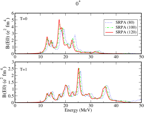
Figure 1: (Color online) Isoscalar (upper panel) and isovector (lower panel) strength distributions for monopole states obtained in SRPA for increasing values of the energy cutoff, indicated in MeV in parenthesis in the figure, on the $2p2h$ configurations.

This means that the ground state is not anymore a Slater determinant. Due to this, the use of the HF ground state to calculate the matrix elements (QBA) is a stronger approximation than in RPA. Extensions to cure this problem in the context of SRPA have been proposed and applied to a simple model srpalipkin and to metal clusters gamba . Future applications to nuclei are in progress.

III Stability of the results and sum rules

In this Section we briefly discuss some technical details of the calculations paying particular attention to the convergence of the results. As a first step, we have solved the HF equation in the coordinate space, by using a 20-fm box. In RPA and SRPA calculations we consider the first $n=7$ single particle (s.p.) states for each $l$, with $l$ up to $6$. The s.p. wavefunctions have been represented as linear superposition of square well ones. The SGII sgii parametrization of the effective interaction has been used in the present calculations. Since Coulomb and spin-orbit are not taken into account in the residual interaction, our calculations are not fully self-consistent and thus violations of the EWSR are found (being at worse of $5\%$). The s.p. space has been chosen large enough to assure that the EWSR are stable. In the following we will focus our attention on the excitation spectrum up to 50 MeV.

In RPA calculations, $1p1h$ configurations with unperturbed energy up to 100 MeV are considered, while in the SRPA ones, we have considered all the $2p2h$ configurations with an unperturbed energy lower than an energy cutoff $E_{cut}$. Due to the ultraviolet divergence related to the zero-range of the interaction, results are not expected to converge with respect to the energy cutoff. We have however checked that they do not change too drastically in the energy regions we are interested in. In order to study the stability of the results with respect to the cutoff, we have analyzed how the strength distributions change by increasing $E_{cut}$ starting from 80 MeV up to 120 MeV. In Figs. 1 and 2 we show the monopole and quadrupole strength distributions, respectively, for different choices of $E_{cut}$ (indicated in MeV in parenthesis in the figures). We see that in both cases a cutoff equal to 120 Mev is suitable to have stable results. Similar stability checks have been systematically made for all the results shown in the article.

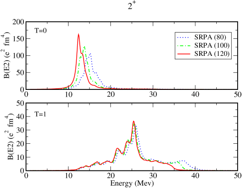
Figure 2: (Color online) As in Fig. 1 but for the quadrupole case.

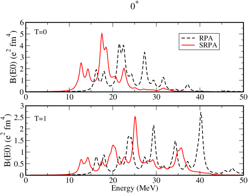
Figure 3: (Color online) RPA, dashed (black) lines and SRPA, full (red) lines, for the isoscalar (upper panel) and isovector (lower panel) monopole strength distributions.

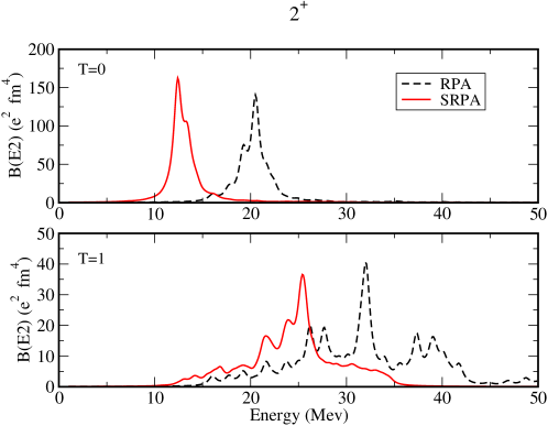
Figure 4: (Color online) As in Fig. 3 but for the quadrupole case.

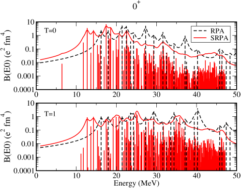
Figure 5: (Color online) As in Fig. 3 but using a logarithmic scale in the ordinate.

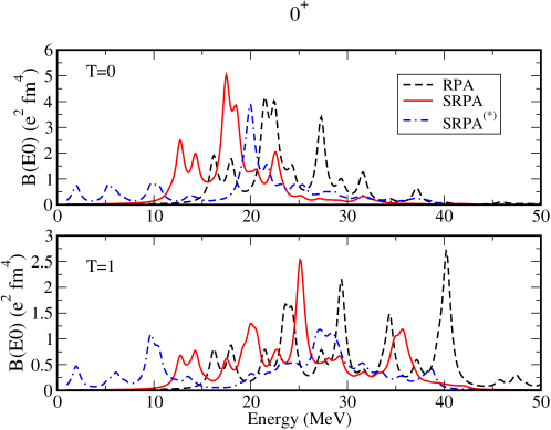
Figure 6: (Color online) Comparison between RPA, dashed (black) lines, SRPA in full (red) lines and SRPA with rearrangements terms, dot-dashed (blue) lines. The isoscalar (upper panel) and isovector (lower panel) monopole strength distributions are shown.

.

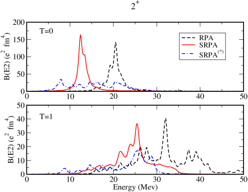
Figure 7: (Color online) As in Fig. 8 but for the quadrupole case.

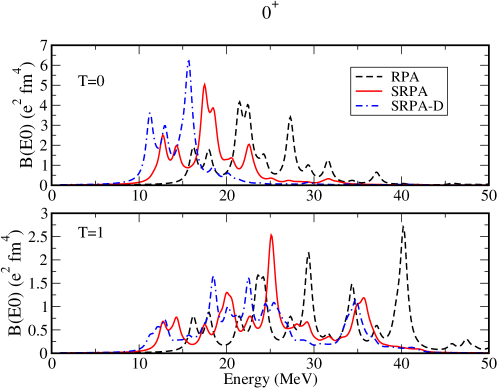
Figure 8: (Color online) Comparison between RPA, dashed (black) lines, SRPA in full (red) lines and SRPA in the diagonal approximation, dot-dashed (blue) lines. The isoscalar (upper panel) and isovector (lower panel) monopole strength distributions are shown.

.

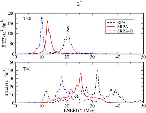
Figure 9: (Color online) As in Fig. 8 but for the quadrupole case.

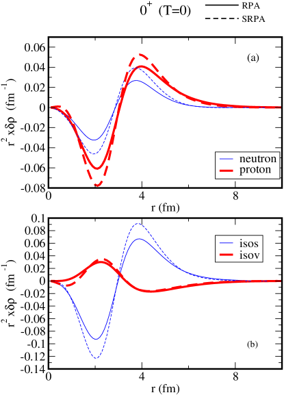
Figure 10: (Color online) Comparison between RPA (full lines) and SRPA (dotted lines) transition densities for the monopole isoscalar states (see text): in the panel (a) neutron (thin lines) and proton (bold lines) parts, while in panel (b) the isoscalar (thin lines) and isovector (bold lines) ones. See text for more details.

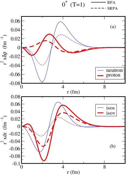
Figure 11: (Color online) As in Fig. 10 but for the monopole isovector states.

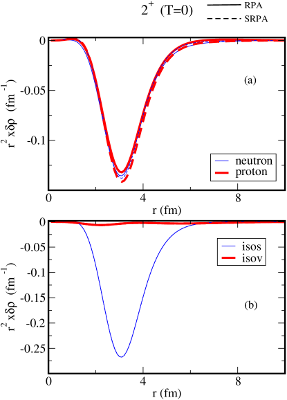
Figure 12: (Color online) Comparison between RPA (full lines) and SRPA (dotted lines) transition densities for the quadrupole isoscalar states (see text): in the panel (a) neutron (thin lines) and proton (bold lines) parts, while in panel (b) the isoscalar (thin lines) and isovector (bold lines) ones. See text for more details.

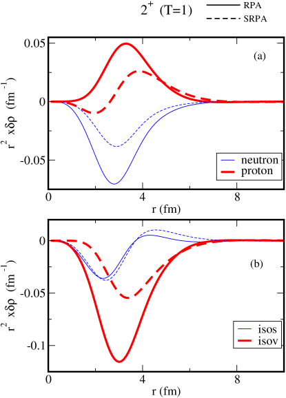
Figure 13: (Color online) As in Fig. 12 but for the quadrupole isovector case.

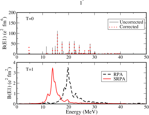
Figure 14: (Color online) Upper panel: SRPA isoscalar dipole strength distribution using a transition operator of radial form $(\sim r^{3})$, full (black) lines and its corrected in dotted (red) lines form $\sim r^{3}-\frac{5}{3}\langle r^{2}\rangle r$ in order to take into account CM corrections. Lower panel: RPA, dashed (black) line and SRPA in full (red) line isovector dipole strength distribution using the standard dipole transition operator of radial form $(\sim r)$.

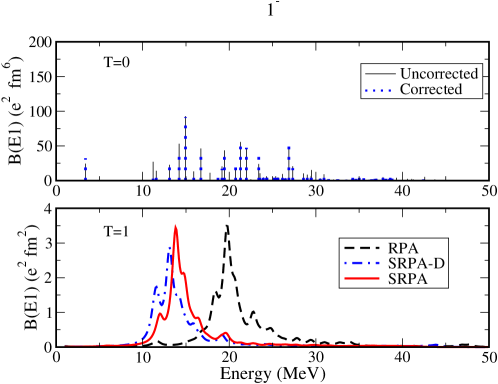
Figure 15: (Color online) Upper panel: isoscalar dipole strength distribution obtained within the SRPA in the diagonal approximation using a transition operator of radial form $(\sim r^{3})$, full (black) lines and its corrected dotted (blue) lines form $\sim r^{3}-\frac{5}{3}\langle r^{2}\rangle r$ in order to take into account CM corrections. Lower panel: RPA, dashed (black) line, SRPA in the diagonal approximation, dot-dashed (blue) line and full SRPA in full (red) line isovector dipole strength distribution using the standard dipole transition operator of radial form $(\sim r)$.

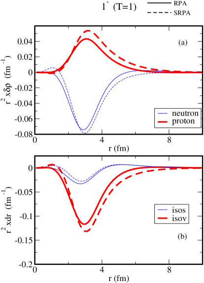
Figure 16: (Color online) As in Fig. 12 but for the dipole isovector case.

As mentioned above, the EWSR are satisfied in SRPA and the first moment (6) is the same in RPA and SRPA. For a generic one body operator,

$$F=\sum_{\alpha,\beta}\langle\alpha\mid F\mid\beta\rangle a_{\alpha}^{\dagger}a_{\beta},$$ (10)

the transition amplitudes are easily calculated and they have the same expression both in RPA and SRPA, namely

$$\langle 0\mid[Q_{\nu},F]\mid 0\rangle\approx\langle HF\mid[Q_{\nu},F]\mid HF\rangle=$$

$$=\sum_{ph}\bigg{\{}X_{ph}^{\nu*}\langle p\mid F\mid h\rangle+Y_{ph}^{\nu*}\langle h\mid F\mid p\rangle\bigg{\}}.$$ (11)

We note that only the $p-h$ components of the transition operator are selected and that, also in the case of the SRPA, only the $1p1h$ amplitudes appear in the above equation.

In the present work, when a energy cutoff $E_{cut}=120$ Mev on the $2p2h$ configurations is used, SRPA calculations involve the diagonalization of large matrices, of the order of $N=5-6\times 10^{4}$ . A Krylov-Schur iteration procedure from the SLEPC package slepc has been used. Since we are interested in the low part of the spectrum, in order to reduce the time of calculation only the first $n$ eigenvalues (with $n\sim 1-2\times 10^{3}$) are calculated. In the evaluation of the first moment (6) we need to know all the excited states and SRPA calculations with high $2p2h$ configurations energy cutoff would require a very long calculation time. Therefore, we have done some calculations with a smaller energy cutoff, i.e., $E_{cut}=60$ MeV so that all the energy spectrum can be calculated. In Table 1 we report, for the monopole case, the isoscalar and isovector values , second and third columns respectively, of the SRPA first moment

$$m_{1}=\sum_{\nu}^{\omega_{max}}\omega_{\nu}|\langle\nu\mid F\mid 0\rangle|^{2}$$ (12)

by including all the states with an excitation energy lower than $\omega_{max}$, whose increasing values are shown in the first column of the table. In the last row, the corresponding RPA values are reported with $\omega_{max}=100$ MeV. We see that, by increasing the value of the parameter $\omega_{max}$, the SRPA values of the first moment obtained in SRPA get close to the RPA ones. Similar results have been obtained also in the quadrupole and dipole cases.

We stress that, even for smaller values of the energy cutoff $E_{cut}$, a similar (almost identical) agreement of the SRPA $m_{1}$ value with the RPA one is found. Indeed, by changing the energy cutoff $E_{cut}$ only a redistribution of the strength is observed while the total strength is the same and is equal to the RPA one. This is related from one hand to the fact that only the $1p1h$ amplitudes appear in the transition amplitudes and on the other hand to the formal properties of the SRPA equations Adachi88 .

	$m_{1}(T=0)$	$m_{1}(T=1)$
$\omega_{max}$ (MeV)	SRPA	SRPA
40	626.4381	115.4153
50	648.9699	147.8026
60	661.0194	182.7364
70	664.3803	193.7896
80	669.7185	197.6874
90	671.4575	200.6472
100	671.6515	201.2473
110	671.6515	201.2473
RPA	671.6516	201.2494

Table 1: Evolution of the monopole isoscalar and isovector first moments obtained in SRPA, second and third columns respectively, as a function of the $\omega_{max}$ parameter (see Eq. 12). In the last row, the corresponding RPA values are reported with $\omega_{max}=100$ MeV.

IV SRPA excitation spectrum in ¹⁶O

In this Section we present the nuclear strength distributions obtained in SRPA for different multipolarities and we compare them with the RPA ones. The doubly magic nucleus ¹⁶O has been chosen for these first applications of Skyrme-SRPA. At SRPA level different levels of approximation will be considered. As discussed above, in the case of density-dependent interactions it is not clear how to define the residual interaction appearing in the matrix elements beyond RPA, in particular as far as the rearrangement terms are concerned. In what follows two possibilities have been explored: (i) first, the interaction is used without rearrangement terms in beyond RPA matrix elements; (i) then, rearrangement terms are included in beyond RPA matrix elements, calculated with the usual RPA prescription.

Furthermore, the full SRPA calculations are compared with the ones obtained when the diagonal approximation is used.

IV.1 Monopole and Quadrupole Strength Distributions

In this subsection we focus our attention on the monopole and quadrupole strength distributions. Unless otherwise stated, no rearrangement terms are included in SRPA calculations. In Fig. 3 we show the RPA (dashed black lines) and SRPA (full red lines) results for the isoscalar (upper panel) and isovector (lower panel) monopole strength distributions. In SRPA all the $2p2h$ configurations with an unperturbed energy lower than an energy cutoff $E_{cut}=120$ MeV are included.

In both isoscalar and isovector cases the strongest effect in SRPA is a several-MeV shift of the strength distribution to lower energies with respect to RPA. This result seems to be a general feature of SRPA and has been found also in different SRPA calculations roth1 ; roth2 ; gamba . A different structure in RPA and SRPA strength distribution is also found not leading, however, to different widths of the peak profiles in SRPA with respect to RPA.

The same remarks are valid also for the quadrupole case displayed in Fig. 4.

Fig. 5 gives an idea about how in detail SRPA describes the fine structure of the response: a very dense distribution of discrete contributions can be seen for the SRPA case due to the existence of many $2p2h$ elementary excitations in addition to the standard RPA $1p1h$ ones.

Figs. 6 and 7 represent the same quantities as Figs. 3 and 4, respectively. However, this time also the SRPA results obtained with rearrangement terms in beyond RPA matrix elements (SRPA^(∗)) are presented in order to evaluate their effect.

For the isoscalar monopole case (top panel of Fig. 6) the residual interaction seems to be more repulsive when rearrangement terms are added providing a smaller energy shift to lower energies with respect to RPA. In all the other cases shown in Figs. 6 and 7, the strength distribution appears very strongly fragmented when rearrangement terms are included in all matrix elements. We know that the adopted way to evaluate the rearrangement terms in beyond RPA matrix elements is not the correct one even if it is currently used. Work is in progress to obtain the correct expressions: the fact that the SRPA^(∗) results are so different from the SRPA ones underlines that this is a very delicate point and indicates that the proper expressions are needed.

In Figs. 8 and 9 the comparison is done with the diagonal approximation. The results are quite different and this suggests that the residual interaction should not be neglected in the matrix $A_{22}$ in Skyrme-SRPA calculations.

Finally, Figs. 10 to 13 display the transition densities. In Fig. 10 (for the monopole isoscalar response) the SRPA transition density refers to the peak at $\sim$ 17 MeV while the RPA transition density is evaluated for the peak at $\sim$ 21 MeV in top panel of Fig. 3. The profiles are not very different meaning that the nature of these RPA and SRPA excited states is not very different in terms of the spatial distributions of wave functions contributing to them. The same considerations can be done for the results shown in Fig. 12 (referring to the quadrupole isoscalar response). In this figure, the RPA (SRPA) transition density is calculated for the peak at $\sim$ 22 MeV (13 MeV) in top panel of Fig. 4.

Different is the case for the isovector responses. In Fig. 11 the RPA (SRPA) transition density, for the monopole response, is calculated for the peak at $\sim$ 29 MeV (25 MeV) shown in the bottom panel of Fig. 3. For the quadrupole case, the transition density obtained in the RPA (SRPA) for the peak at $\sim$ 32 MeV (25 MeV), (see lower panel of Fig. 4), are shown in Fig. 13.

Important differences are visible between RPA and SRPA suggesting that the nature of SRPA and RPA excited states in terms of radial distribution of wave functions contributing to the excitation is quite different.

IV.2 Dipole Strength Distributions

The Thouless theorem on the EWSR thou is a very important feature of RPA and it holds also in SRPA Yannouleas . It guarantees that spurious excitations corresponding to broken symmetries separate out and are orthogonal to the physical states. In Ref. SchuckSS a detailed discussion about the treatment of single and double spurious modes in RPA and extended RPA theories has been presented. In particular, it has been shown that, when an approximate ground state is used and/or $2p2h$ configurations are included, all the single-particle amplitudes have to be taken into account for the construction of the elementary configurations in order to have single and double spurious modes lying at zero energy. In a self-consistent RPA, i.e., when the same interaction is used at HF and RPA level, the motion of the center of mass (associated with the translational invariance) appears at zero energy being thus exactly separated from the physical spectrum. As mentioned above, our RPA approach is not fully self-consistent and the spurious state lies at about 1 MeV exhausting more than 96% of the isoscalar EWSR. In SRPA, as a consequence of the coupling with the $2p2h$ configurations, the spurious state is found to be at imaginary energy. We stress that in a self-consistent SRPA approach this state should appear at zero energy as in RPA. In order to study the possible mixing with spurious components, we have examined the isoscalar dipole strength distribution using a transition operator of the radial form $(\sim r^{3})$ and its corrected form $(\sim r^{3}-\frac{5}{3}\langle r^{2}\rangle r)$. The results are shown in the upper panel of Fig. 14. We can see that some differences between the two cases appear, especially in the lowest part of the spectrum, while the mixing with spurious components is smaller in the energy region around and beyond the isovector dipole giant resonance. We remind that a prescription often used in the literature for the treatment of the spurious mode consists in multiplying the residual interaction by a renormalizing factor such that the spurious mode is found at zero energy. In our RPA calculations the spurious state is found at 1.02 MeV and by using a renormalizing factor of 1.006 its energy goes down to 0.02 MeV; the rest of the isoscalar and isovector distributions remain practically unchanged. The same prescription has not been used in SRPA since the use of a renormalizing factor does not solve the problem of the appearance of imaginary solutions, even when larger values of the renormalizing factor are used.

In the lower panel of Fig. 14 we plot the results for the isovector case, with the excitation operator $(\sim r)$. We observe that going from RPA to SRPA, as in the monopole and quadrupole cases, a strong shift towards lower energies of the strength distribution.

In Fig. 15 we show the results when the diagonal approximation is used. In the upper panel of the figure, the isoscalar strength distributions using the corrected and uncorrected transition operator are shown and we see that, as in the previous case, very small differences are present when the two different operators are used. In the lower panel of the same figure, the isovector distributions obtained in RPA (dashed-black line), SRPA in the diagonal approximation (dot-dashed blue line) and full SRPA (full-red line) are shown. It is interesting to note that the results obtained in the diagonal approximation are different from the ones obtained in the full SRPA, the differences however being smaller than the ones found in the monopole and quadrupole cases.

As far as the rearrangement terms are concerned, we have found in the dipole case that, even when small values of the $2p2h$ energy cutoff $E_{cut}$ are used (60-80 MeV), the SRPA equations give imaginary solutions if the rearrangement terms are included in all matrix elements. Moreover, by comparing in this case the isoscalar strength distributions obtained by using the corrected and uncorrected transition operator, very large differences are found, especially in the low energy part of the spectrum, indicating that a strong mixing with spurious components is present in this case. In the isovector channel, the position of the main peak is not very different from the one obtained when no rearrangement terms are used (lower panel of Fig. 14) but the height of the peak is strongly reduced (more than 50%).

In Fig. 16 the RPA (SRPA) transition density, for the isovector dipole response, is calculated for the peak at $\sim$ 20 MeV (14 MeV) shown in the bottom panel of Fig. 14. We see that in the dipole case the transition densities in RPA and SRPA are quite similar. This behaviour is at variance from what we found in the monopole and quadrupole cases, as sown in Figs 11 and 13, respectively.

IV.3 Low-lying 0⁺ and $2^{+}$ states

The results for the 0⁺ and $2^{+}$ low-lying states obtained in SRPA are shown in Tables 2 and 3. These states are mainly composed by $2p2h$ configurations.

The largest $1p1h$ configuration in the $0^{+}$ state is $(2p_{\frac{1}{2}},1p_{\frac{1}{2}})^{\pi}$ with an unperturbed energy of 16.17 Mev when no rearrangement terms are considered and $(3p_{\frac{1}{2}},1p_{\frac{1}{2}})^{\nu}$ with an unperturbed energy of 24.03 MeV when rearrangement terms are included. In both cases, the lowest $2p2h$ configuration is $\big{[}[1d_{\frac{5}{2}},1p_{\frac{1}{2}}]^{3}[(1d_{\frac{5}{2}},1p_{\frac{1}{2}}]^{3}\big{]}_{\pi}^{0}$ with an unperturbed energy of E=15.26 MeV.

For the $2^{+}$ state the most important $1p1h$ configuration is $(2d_{\frac{5}{2}},1s_{\frac{1}{2}})^{\pi}$ with an unperturbed energy of 28.28 MeV when rearrangement terms are not considered. When rearrangement terms are included the most important configuration is $(2p_{\frac{3}{2}},1p_{\frac{1}{2}})^{\nu}$ with an unperturbed energy of 21.71 MeV. The lowest $2p2h$ configuration is, in both cases, $\big{[}[1d_{\frac{5}{2}},1p_{\frac{1}{2}}]^{3}[(1d_{\frac{5}{2}},1p_{\frac{1}{2}}]^{3}\big{]}_{\pi}^{2}$ with an unperturbed energy of 15.26 MeV.

Low Lying $0^{+}$ energy (MeV)
Exp	RPA	SRPA	SRPA-D	SRPA∗	SRPA∗-D
$\sim$6	16.19	6.43	11.23	5.29	Imm.

Table 2: Energy of the lowest $0^{+}$ state obtained in RPA and in SRPA, compared with the experimental value Low0p2p . The results identified with the star are obtained by taking into account rearrangement terms (last two rows). With “SRPA-D” we indicate the SRPA results when the diagonal approximation is used (fourth and sixth rows). The SRPA result in the diagonal approximation whit rearrangement terms gives imaginary solution (last row).

Low Lying $2^{+}$ energy (MeV)
Exp	RPA	SRPA	SRPA-D	SRPA∗	SRPA∗-D
$\sim$7	16.03	7.16	12.44	4.70	Imm.

Table 3: As in Table 2 but for $2^{+}$ state.

Several conclusions may be drawn about these results. First, RPA is not at all able to describe these low-lying states simply because beyond $1p1h$ configurations are necessary to construct them. RPA energies are indeed far too high in both cases.

It is striking that the SRPA energies are very close to the experimental results. The residual interaction seems to be very important for describing these states: the first unperturbed $2p2h$ configuration is actually located at about 15 MeV and the residual interaction is thus responsible for the strong shift to lower energies in the response. When rearrangement terms are included, the shift is even stronger.

The diagonal approximation looks very poor for the treatment of these low-energy states indicating that the interaction between $2p2h$ configurations is very important for providing the correct excitation energies.

Finally, it can be interesting to compare the SRPA results with other types of analysis. As an illustration, let us consider the energy of the first 0⁺ excited state. Ab-initio coupled cluster investigations do not reproduce at all the energy of this state providing an excitation energy of 19.8 MeV wl . Brown and Green have described the low-lying states in ¹⁶O by mixing spherical and deformed states br . Shell model can nicely describe these states due to the configuration mixing zu . Cluster models are also able to well describe this state by assuming an $\alpha$+¹²C or a 4$\alpha$ structure for the nucleus ¹⁶O (see Ref. fu and references therein). SRPA is the only RPA-like approach in spherical symmetry that reproduces this energy without any special modelization for the structure of the nucleus ¹⁶O.

It is worth mentioning however that a complete analysis of these low energy states would need also the evaluation of the B(E$\lambda$) values. Work is in progress in this direction to evaluate the transition probabilities in these cases where the excitations are mainly composed by $2p2h$ configurations.

V Conclusions

We have performed Skyrme-SRPA calculations for describing collective and low-lying excited states in ¹⁶O. The Skyrme interaction SGII is used. The SRPA scheme is fully treated without employing the currently used Second-Tamm-Dancoff or diagonal approximations. The rearrangement terms of the residual interaction are treated in this work (i) by neglecting them in the matrix elements beyond RPA; (ii) by calculating them with the usual RPA procedure for all the matrix elements. Work is in progress to derive the proper expressions to be used in beyond RPA matrix elements.

A general feature of the SRPA spectra is a several-MeV shift to lower energies with respect to RPA distributions. This shift being very strong, Skyrme-SRPA energies of giant resonances are typically too low with respect to the experimental response (Skyrme-RPA results are in general in good agreement with the experimental data for these excitations). To cure this problem we plan to explore the possibility of using an extended SRPA scheme in the same line of Ref. gamba ; gamba2010 . A longer term project is to look for some new parametrization of the effective interaction, adjusted so to make it suitable for this kind of calculations

The SRPA energies of the low-lying 0⁺ and 2⁺ states are in very good agreement with the experimental results. Work is in progress to evaluate the transition probabilities and complete the analysis of these excitation modes.

Finally, after this first numerical application of the method, we plan in future works to explore with SRPA heavier or more exotic nuclei and to check the model dependence of the results by employing also other Skyrme parametrizations.

- (1) P. Ring and P. Schuck, The nuclear Many-Body Problem, Springer-Verlag Berlin Heidelberg New York, 1980; E. Khan, N. Sandulescu, M. Grasso, and N. Van Giai, Phys. Rev. C 66, 024309 (2002)
- (2) D. Gambacurta, F. Catara, and M. Grasso, Phys. Rev. C 80, 014303 (2009)
- (3) C. Yannouleas, Phys. Rev. C 35, 1159 (1986)
- (4) J. da Providencia, Nucl. Phys. 61, 87 (1965)
- (5) M. Tohyama and M. Gong, Z. Phys. A 332, 269 (1989)
- (6) D. Lacroix, S. Ayik, and Ph. Chomaz, Prog. Part. Nucl. Phys. 52, 497 (2004)
- (7) T. Hoshino and A. Arima, Phys. Rev. Lett. 37, 266 (1976)
- (8) W. Knupfer and M.G. Huber, Z. Phys. 276, 99 (1976)
- (9) S. Nishizaki and J. Wambach, Phys. Lett. B 349, 7 (1995)
- (10) S. Nishizaki and J. Wambach, Phys. Rev. C 57, 1515 (1998)
- (11) S. Adachi and S. Yoshida, Nucl. Phys. A 306, 53 (1978)
- (12) B. Schwesinger and J. Wambach, Phys. Lett. B 134, 29 (1984)
- (13) B. Schwesinger and J. Wambach, Nucl. Phys. A 426, 253 (1984)
- (14) S. Drozdz, V. Klent, J. Speth, and J. Wambach, Nucl. Phys. A 451, 11 (1986)
- (15) S. Drozdz, V. Klent, J. Speth, and J. Wambach, Phys. Lett. B 166, 18 (1986)
- (16) C. Yannouleas, M. Dworzecka, and J.J. Griffin, Nucl. Phys. A 397, 239 (1983)
- (17) C. Yannouleas and S. Jang, Nucl. Phys. A 455, 40 (1986)
- (18) P. Papakonstantinou and R. Roth, Phys. Lett. B 671, 356 (2009)
- (19) P. Papakonstantinou and R. Roth, arXiv:0910.1674v1 [nucl-th]
- (20) D. Gambacurta and F. Catara, Phys. Rev. B 79, 085403 (2009)
- (21) N. Van Giai and H. Sagawa, Phys. Lett. 106B 379 (1981); N. Van Giai, N. Sagawa, Nucl. Phys. A 371 1 (1981).
- (22) E. Litvinova, P. Ring and V. Tselyaev, Phys. Rev. C 78, 14312 (2008); G. Tertychny, V. Tselyaev, S. Kamerdzhiev, F. Krewald, J. Speth, E. Litvinova and A. Avdeenkov, Nucl. Phys. A 788, 159 (2007); G. Coló, H. Sagawa, N. Van Giai, P. F. Bortignon and T. Suzuki, Phys. Rev. C 57, 3049 (1998); G. Colò, N. Van Giai, P. F. Bortignon and R. A. Broglia, Phys. Rev. C 50, 1496 (1994)
- (23) Ph. Chomaz and N. Frascaria, Phys. Rep. 252, 275 (1995); K. Boretzsky, et al., Phys. Rev. C 68, 024317 (2003); M. Fallot, et al., Nucl. Phys. A 729, 699 (2003)
- (24) E. Lanza, F. Catara, D. Gambacurta, M.V. Andrés, and Ph. Chomaz, Phys. Rev. C 79, 054615 (2009)
- (25) S. Adachi and S. Yoshida, Phys. Lett. B 81, 98 (1978)
- (26) S. Adachi and S. Yoshida, Nucl. Phys. A 462, 61 (1987)
- (27) S. Adachi, E. Lipparini, Nucl. Phys. A489, 445 (1988)
- (28) G. Lauritsch and P. G. Reinhard, Nucl. Phys. A509, 287 (1990); K. Takayanagi, K. Shimizu and A. Arima, Nucl. Phys. A477, 205 (1988); A. Mariano, F. Krmpotic and A. F. R. de Toledo Piza, Phys. Rev. C49, 2824 (1994).
- (29) D. Gambacurta, M. Grasso, F. Catara, and M. Sambataro, Phys. Rev. C 73, 024319 (2006)
- (30) A Scalable and Flexible Toolkit for the Solution of Eigenvalue Problems, Vicente Hernandez and Jose E. Roman and Vicente Vidal, ACM Transactions on Mathematical Software, 31, 3, 351 362,2005 http://www.grycap.upv.es/slepc
- (31) D. J. Thouless, Nucl. Phys. 21, 225 (1960).
- (32) M. Tohyama and P. Schuck, Eur. Phys. J. A19, 203 (2004);
- (33) F. Ajzenberg-Selove, Nucl. Phys. A375, 1 (1982); O. Sorlin and M. G. Porquet, Progress in Part. and Nucl. Phys. 61, 602 (2008)
- (34) M. Wloch, et al., Phys. Rev. Lett. 94, 212501 (2005)
- (35) G.E. Brown and A.M. Green. Nucl. Phys. 75, 401 (1966)
- (36) A.P. Zuker, B. Buck and J.B. McGrory. Phys. Rev. Lett. 21, 39 (1968)
- (37) Y. Funaki, et al., Phys. Rev. Lett 101, 082502 (2008)
- (38) D. Gambacurta and F. Catara, Phys. Rev. B 81, 085418 (2010)