Magnetoasymmetric transport in a mesoscopic interferometer: From the weak to the strong coupling regime

Abstract

The microreversibility principle implies that the conductance of a two-terminal Aharonov-Bohm interferometer is an even function of the applied magnetic flux. Away from linear response, however, this symmetry is not fulfilled and the conductance phase of the interferometer when a quantum dot is inserted in one of its arms can be a continuous function of the bias voltage. Such magnetoasymmetries have been investigated in related mesoscopic systems and arise as a consequence of the asymetric response of the internal potential of the conductor out of equilibrium. Here we discuss magnetoasymmetries in quantum-dot Aharonov-Bohm interferometers when strong electron-electron interactions are taken into account beyond the mean-field approach. We find that at very low temperatures the asymmetric element of the differential conductance shows an abrupt change for voltages around the Fermi level. At higher temperatures we recover a smooth variation of the magnetoasymmetry as a function of the bias. We illustrate our results with the aid of the electron occupation at the dot, demonstrating that its nonequilibrium component is an asymmetric function of the flux even to lowest order in voltage. We also calculate the magnetoasymmetry of the current–current correlations (the noise) and find that it is given, to a good extent, by the magnetoasymmetry of the weakly nonlinear conductance term. Therefore, both magnetoasymmetries (noise and conductance) are related to each other via a higher-order fluctuation-dissipation relation. This result appears to be true even in the low temperature regime, where Kondo physics and many-body effects dominate the transport properties.

I Introduction

Transport in electric conductors is governed by fundamental principles when the fields applied to the system are small. For instance, in the linear regime microscopic reversibility leads to symmetric response coefficients, as demonstrated by Onsager.ons In the case of a conductor coupled to two terminals, the linear conductance $G_{0}$ is an even function of the magnetic field $B$.cas When the conductor is reduced to typical sizes less than the phase-breaking length, electron mesoscopic transport depends on the particular arrangement of the attached probes in a multiterminal configuration in such a way that current and voltage terminals must be exchanged to recover the Onsager symmetry.but86 On the other hand, in the mesoscopic regime interference effects associated to the wave nature of carriers can be detected in a transport measurement. A prominent example is an Aharonov-Bohm interferometer with a quantum dot inserted in one of its arms for which the linear conductance $G_{0}$ is periodically modulated by the externally applied flux. However, the conductance phase $\delta$, which can be related to the transmission phase through the quantum dot, shows abrupt jumps as a function of the gate voltageyac95 since the Onsager symmetry establishes that $\delta$ can be $0$ or $\pi$ only.lev95 Further theoreticalhac96 ; bru96 and experimental worksyac96 ; shu97 have addressed the effect of electron-electron interactions inside the quantum dot.

Away from linear response, the principle of microscopic reversibility is, generally, not satisfied and, as a consequence, the two-terminal current, which consists of linear as well as nonlinear coefficients, is not a symmetric function of $B$. Recently, this magnetoasymmetry effect has been theoretically demonstrated san04 ; spi04 ; but05 ; san05 ; pol06 ; mart06 ; and06 ; pol07 ; san08 ; kal09 ; sza09 ; her09 and experimentally verified rik05 ; wei06 ; mar06 ; let06 ; zum06 ; ang07 ; har08 ; che09 ; bra09 . Magnetoasymmetries arise because the charge response of the system is, generally, not symmetric when the field orientation is inverted.san04 ; spi04 Out of equilibrium, the piled-up charge injected from the external reservoirs is partly balanced by the screening potential of the conductor. This internal potential is not an even function of $B$ (the Hall potential is a paradigmatic example)san04 , leading to magnetoasymmetries seen already in the secod-order coefficients within an expansion of currents in powers of voltages.san04 Now, computation of the internal potential due to long range Coulomb interaction is a difficult task and requires self-consistency. This calculation can be achieved within a mean-field scheme, as previous works have done.san04 ; spi04 ; but05 ; san05 ; pol06 However, the importance of strong electron-electron correlations such as those giving rise to the Kondo effecttheoretical ; experimental has not been clarified yet. This is the goal we want to accomplish in this work.

Our calculations are also relevant in view of recent developments that relate the magnetoasymmetries of the current and that of the noise to leading order in a voltage expansion.foe08 ; sai08 ; san09 ; uts09 It has been shown that novel fluctuations relations hold in the weakly nonlinear regime between the asymmetric second-order conductance and the first-order noise susceptibility in terms of a higher-order fluctuation-dissipation theorem. These works explicitly check this relation for specific systems by treating interactions in the mean-field limit.foe08 ; sai08 ; san09 ; uts09 Thus, it is highly desirable to find systems in which the nonequilibrium fluctuation relations can be checked beyond the mean-field case.

We here consider a quantum dot embedded in one of the arms of a two-terminal mesoscopic interferometer. We employ the nonequilibrium Keldysh Green function formalism to describe the transport properties of the system and use an equation-of-motion technique to calculate both the current and the noise in the nonlinear regime including electron-electron correlation terms not present in the Hartree-Fock (mean-field) approximation.

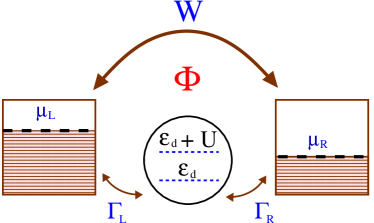
Figure 1: (Color online) Sketch of a mesoscopic interferometer with a quantum dot inserted in the lower arm.

The oscillations in the conductance of an Aharonov-Bohm ring occur in the mesoscopic regime, where the electrons’ phase coherence is preserved. Interference takes place between electron waves that pick up different phases while traversing the two arms of the interferometer even if the electron does not directly experience the flux enclosed by the ring. When a finite bias is applied, the phase of the differential conductance shows a continuous variation with $B$ since the Onsager symmetry need not hold away from linear response.bru96 ; kon02 ; wie03 Such phase rigidity breakings have been recently related to the onset of inelastic cotunneling of a Coulomb-blockaded quantum dot placed in one of the arms.sig07 ; pul09 The effect is rather generic as the phase symmetry can be also broken using microwave fieldssun99 or coupling to phonons.rom07

We now give a simple argument that sheds light on the appearance of magnetoasymmetries in a quantum-dot Aharonov-Bohm ring. A sketch of the system is depicted in Fig. 1. We model the interaction in the dot with an on-site charging energy $U$. We assume for simplicity that the dot contains a single energy level $\varepsilon_{d}$ which acquires a finite lifetime $2\hbar/\Gamma$ due to coupling to the external reservoirs. Then, within the Hartree approximation for the Anderson Hamiltoniananderson the (retarded) Green function for dot electrons with spin $\sigma$ reads,

$$G_{d\sigma}^{r}(\omega)=\frac{1}{\omega-\varepsilon_{d}-U\langle n_{d\bar{\sigma}}\rangle+\frac{1}{4}\sqrt{{\cal{T}}_{b}}\Gamma\cos\left(\frac{e\Phi}{\hbar}\right)+\frac{i}{2}\widetilde{\Gamma}}\,,$$ (1)

where $\widetilde{\Gamma}$ renormalizes $\Gamma$ due to the presence of the nonresonant channel (the upper arm in Fig. 1). Its (energy-independent) transmission is denoted with ${{\cal{T}}_{b}}$. Importantly, the renormalization of the level $\varepsilon_{d}$ is given by two terms. The term that explicitly depends on ${{\cal{T}}_{b}}$ is an even function of the magnetic flux $\Phi$ and it fulfills the Onsager symmetry. However, the term $U\langle n_{d\bar{\sigma}}\rangle$, proportional to the interaction strength, is generally not symmetric under field reversal since the dot occupation $\langle n_{d\bar{\sigma}}\rangle$ out of equilibrium need not fulfill the Onsager symmetry.

Let us expand the dependence of $\langle n_{d\bar{\sigma}}\rangle$ on the external bias $V$ in powers of $V$,

$$\langle n_{d\bar{\sigma}}\rangle=\langle n_{d\bar{\sigma}}\rangle^{(0)}+\langle n_{d\bar{\sigma}}\rangle^{(1)}V+{\cal{O}}(V)^{2}\,.$$ (2)

$\langle n_{d\bar{\sigma}}\rangle^{(0)}$ is the equilibrium charge and must be $B$-symmetric. The nonequilibrium response of the dot to leading order in $V$ is given by $\langle n_{d\bar{\sigma}}\rangle^{(1)}=\partial\langle n_{d\bar{\sigma}}\rangle/\partial V|_{V=0}$. $\langle n_{d\bar{\sigma}}\rangle^{(1)}$ is then determined from the change in the dot occupation when a small shift is applied to the leads’ electrochemical potential. Hence, $\langle n_{d\bar{\sigma}}\rangle^{(1)}$ is a charge susceptibility that includes information about the screening properties of the dot and, as such, must be computed self-consistently in the presence of $V$ (e.g., from charge-neutrality condition).christen We below show that processes of charge filling of the dot from the left lead contribute to the occupation with a term proportional to $1+\sqrt{{\cal{T}}_{b}}\sin(e\Phi/\hbar)$ whereas the contribution from the right lead is proportional to $1-\sqrt{{\cal{T}}_{b}}\sin(e\Phi/\hbar)$. Clearly, the sine terms are not even under $B$-reversal. As a result, electron transfer from left to right at a given orientation of $B$ does not occur with the same probability that the reverse transfer when the $B$ direction is inverted. In other words, the injectivity from the left, which is the partial density of states associated to carriers injected from the left contact,but93 does not equal the right injectivity under $B$ reversal.san04 As a consequence, one finds $\langle n_{d\bar{\sigma}}\rangle^{(1)}\propto\sqrt{{\cal{T}}_{b}}\sin(e\Phi/\hbar)$. Inserting Eq. (2) in Eq. (1), there arises in the denominator a term proportional to $UV\sqrt{{\cal{T}}_{b}}\sin(e\Phi/h)$, which is responsible, to leading order, for the magnetoasymmetry of the nonlinear conductance. Note that this term vanishes in the absence of interactions ($U=0$) or at equilibrium ($V=0$) in which cases the Onsager symmetry is recovered. This further demonstrates that magnetoasymmetries arise as a consequence of the presence of both interactions and external bias.

The asymmetric behavior discussed here can be verified experimentally. Recent experiments with rings show microreversibility violations in the nonlinear regime. An unexpected even-odd behavior has been revealed by Leturcq et al.let06 In an expansion of the observed current–voltage characteristics, they find that the odd (even) coefficients are symmetric (asymmetric) under reversal of $B$. This is surprising since one would expect all coefficients beyond the linear response to be asymmetric, not only the even ones. Therefore, it is instructive to derive the conductance series expansion. The magnetoasymmetric effect appears in the nonlinear regime only because the internal potential is an asymmetric function of $B$ at finite bias. And this dependence on the internal potential is shown in the even coefficients, not in the odd ones. A mean-field description gives this behaviorlet06 since the dot potential depends linearly with $V$, as can be also inferred from our discussion above. Below, we find that the effect persists even if higher electronic correlations are taken into account.

Microreversibility at linear response also leads to the fluctuation-dissipation theorem, which relates the dissipative part of the electric transport (the linear conductance) to the fluctuations at equilibrium (the thermal noise). Since it is clear that microreversibility is broken beyond the linear response regime, it thus natural to ask whether higher-order fluctuation relations exist in the presence of an external field. We find an approximate verification of such relations to next order in the voltage expansion. In other words, the asymmetric part of the second-order conductance and that of the linear-order noise are related to each order via a nontrivial fluctuation relation. Remarkably, our results are interesting because we treat interactions beyond the Hartree-Fock approximation.

The paper is organized as follows. In Sec. II we introduce the system and its Hamiltonian. Section. III is devoted to the transport properties. We also analyze two approximations: the noninteracting case and the Hartree approach. Both limits have serious drawbacks and can even lead to unphysical predictions but we nevertheless include discuss them for pedagogical reasons. A detailed study of the transport coefficients in the Coulomb blocakde regime is contained in Sec. IV. We examine the even-odd properties of the conductance terms both for zero and nonzero temperatures. In Sec. V we consider the Kondo regime, which is the relevant scenario at very low temperatures. We briefly discuss the limits of temperatures lower and higher than the Kondo temperature and then present numerical results for the magnetoasymmetric differential conductance as a function of the background transmission and bias voltage. In Sec. VI we calculate the noise and show that it is an asymmetric function of the magnetic flux. Finally, our results are summarized in Sec.  VII.

II Theoretical model

The mesoscopic interferometer consists of an Aharonov-Bohm ring with a quantum dot inserted in one of its arms. The interferometer is coupled to left ($L$) and right ($R$) leads with continuous energy spectrum $\varepsilon_{k\sigma}$ where $k$ is the wavevector. An electron can travel either through the nonresonant arm with probability amplitude $W$ or via the quantum dot with hopping terms $V_{\alpha}$ where $\alpha=L,R$ is the contact index. The spin-degenerate level dot is denoted with $\varepsilon_{d}$ and the charging energy is $U$. Finally, the magnetic flux $\Phi$ piercing the ring results in an Aharonov-Bohm phase $\varphi=e\Phi/\hbar$. Hence, the Hamiltonian reads,

$${\cal{H}}={\cal{H}}_{C}+{\cal{H}}_{D}+{\cal{H}}_{T}\,.$$ (3)

Here,

$${\cal{H}}_{C}=\sum_{\alpha=L/R,k,\sigma}\varepsilon_{k\sigma}c_{\alpha k\sigma}^{\dagger}c_{\alpha k\sigma}\\ +\sum_{k,k^{\prime},\sigma}\left(We^{i\varphi}c_{Rk^{\prime}\sigma}^{\dagger}c_{Lk\sigma}+{\rm h.c.}\right)\,,$$ (4)

describes the two leads and the direct channel that couples them. The gauge is chosen in such a way that an electron wave picks up the phase $\varphi$ whenever it passes along the upper arm. The dot electrons obey,

$${\cal{H}}_{D}=\sum_{\sigma}\varepsilon_{d}d_{\sigma}^{\dagger}d_{\sigma}+Un_{d\uparrow}n_{d\downarrow}\,,$$ (5)

while the tunneling Hamiltonian between the reservoirs and the dot is given by,

$${\cal{H}}_{T}=\sum_{\alpha=L/R,k,\sigma}\left(V_{\alpha}c_{\alpha k\sigma}^{\dagger}d_{\sigma}+h.c.\right)\,,$$ (6)

where the tunneling amplitudes $V_{\alpha}$ are asummed to be independent of $k$ for simplicity. The same assumption is made for the direct transmission $W$.

III Transport properties

In the stationary limit, the current $I$ can be calculated from the time evolution of the occupation number of the right contact ($n_{R}$),

$$I=I_{R}=-e\frac{d\langle n_{R}\rangle}{dt}=-\frac{ie}{\hbar}\langle[{\cal{H}},n_{R}]\rangle\,,$$ (7)

where $n_{R}=\sum_{k\sigma}c_{Rk\sigma}^{\dagger}c_{Rk\sigma}$. Using the Keldysh formalism,mei92 the current becomes

$$I=\frac{e}{h}\sum_{p,q,\sigma}\int_{-\infty}^{\infty}d\omega~{}\left[\left(V_{R}{\cal{G}}_{d\sigma,Rq\sigma}^{<}(\epsilon)-V_{R}^{\ast}{\cal{G}}_{Rq\sigma,d\sigma}^{<}(\omega)\right)\right.\\ +\left.\left(We^{i\varphi}{\cal{G}}_{Lp\sigma,Rq\sigma}^{<}(\omega)-W^{*}e^{-i\varphi}{\cal{G}}_{Rq\sigma,Lp\sigma}^{<}(\omega)\right)\right],$$ (8)

with the following definitions for the lesser Green fucntion ($G^{<}$):

$${\cal{G}}_{Lp\sigma,Rq\sigma}^{<} =i\langle c_{Rq\sigma}^{\dagger}c_{Lp\sigma}\rangle\,,$$ (9a)

$${\cal{G}}_{Rq\sigma,Lp\sigma}^{<} =i\langle c_{Lp\sigma}^{\dagger}c_{Rq\sigma}\rangle\,,$$ (9b)

$${\cal{G}}_{d\sigma,Rq\sigma}^{<} =i\langle c_{Rq\sigma}^{\dagger}d_{\sigma}\rangle\,,$$ (9c)

$${\cal{G}}_{Rq\sigma,d\sigma}^{<} =i\langle d_{\sigma}^{\dagger}c_{Rq\sigma}\rangle\,.$$ (9d)

In the case of energy-independent couplings or for proportionate couplings, the expresssion for the current is more conveniently recast in terms of a generalized transmission function ${\cal{T}}_{\sigma}(\omega)$ for an electron with spin $\sigma$ and energy $\omega$,

$$I=-\frac{e}{h}\sum_{\sigma}\int d\omega~{}{\cal{T}}_{\sigma}(\omega)[f_{L}(\omega)-f_{R}(\omega)]\,,$$ (10)

where $f_{L}$ and $f_{R}$ are the Fermi-Dirac distribution functions in the leads $L$ and $R$, respectively. The transmission reads,bul01 ; hof01

$${\cal{T}}_{\sigma}(\omega)={\cal{T}}_{b}+\sqrt{\alpha{\cal{T}}_{b}{\cal{R}}_{b}}\cos(\varphi)\widetilde{\Gamma}\operatorname{Re}\left[{\cal{G}}_{d\sigma,d\sigma}^{r}(\omega)\right]\\ -\frac{1}{2}\left\{\alpha\left[1-{\cal{T}}_{b}\cos^{2}(\varphi)\right]-{\cal{T}}_{b}\right\}\widetilde{\Gamma}\operatorname{Im}\left[{\cal{G}}_{d\sigma,d\sigma}^{r}(\omega)\right]\,.$$ (11)

Here, ${\cal{T}}_{b}$ is the transmission probability between the two leads along the direct channel,

$${\cal{T}}_{b}=\frac{4\xi}{(1+\xi)^{2}}\,,$$ (12)

where $\xi=\pi^{2}W^{2}\rho_{L}\rho_{R}$ with $\rho_{L(R)}$ the density of states for lead $L(R)$. The reflection probability ${\cal{R}}_{b}$ is determined from ${\cal{R}}_{b}=1-{\cal{T}}_{b}$. The broadening of the dot level due to hybridization with states of lead $L(R)$ reads $\Gamma_{L(R)}=2\pi|V_{L(R)}|^{2}\rho_{L(R)}$, where $\rho_{L(R)}$ is the density of states for lead $L(R)$. The total linewidth is $\Gamma=\Gamma_{L}+\Gamma_{R}$. In the wide band limit, we take $\rho_{L(R)}=\rho_{0}$ (and, consequently, $\xi$ and $\Gamma$) to be energy independent. In the presence of the upper bridge, the broadening becomes renormalized,

$$\widetilde{\Gamma}=\frac{\Gamma}{1+\xi}\,,$$ (13)

Finally, the factor $\alpha=4\Gamma_{L}\Gamma_{R}/\Gamma^{2}$ in Eq. (11) quantifies the tunneling asymmetry ($0\leq\alpha\leq 1$). It yields $\alpha=1$ for symmetric couplings ($\Gamma_{L}=\Gamma_{R}=\Gamma/2$).

The problem has thus been reduced to the calculation of the dot retarded Green function ${\cal{G}}_{d\sigma,d\sigma}^{r}(\omega)$. For later convenience, we introduce the following definitions:

$$\langle\langle A(t),B(t^{\prime})\rangle\rangle^{<} =+i\langle B(t^{\prime})A(t)\rangle\,,$$ (14a)

$$\langle\langle A(t),B(t^{\prime})\rangle\rangle^{>} =-i\langle A(t)B(t^{\prime})\rangle\,,$$ (14b)

$$\langle\langle A(t),B(t^{\prime})\rangle\rangle^{r} =-i\Theta(t-t^{\prime})\langle[A(t),B(t^{\prime})]_{+}\rangle\,,$$ (14c)

$$\langle\langle A(t),B(t^{\prime})\rangle\rangle^{a} =+i\Theta(t^{\prime}-t)\langle[A(t),B(t^{\prime})]_{+}\rangle\,,$$ (14d)

where $r$ ($a$) stands for ”retarded” (”advanced”). Using the operators $A=d_{\sigma}$ and $B=d_{\sigma}^{\dagger}$ we obtain the dot Green function,

$${\cal{G}}_{d\sigma,d\sigma}^{r}(\omega)=\int_{-\infty}^{\infty}dt\,e^{i\omega t}\langle\langle d(t),d^{\dagger}(0)\rangle\rangle^{r}\,,$$ (15)

where we have set $t^{\prime}=0$ since the Hamiltonian is time independent. The equation of motion for ${\cal{G}}_{d\sigma,d\sigma}^{r}$ is found as,

$$\left[\omega-\varepsilon_{d}+\frac{1}{4}\sqrt{\alpha{\cal{T}}_{b}}\Gamma\cos(\varphi)+\frac{i}{2}\widetilde{\Gamma}\right]\langle\langle d_{\sigma},d_{\sigma}^{\dagger}\rangle\rangle^{r}=1\\ +U\langle\langle d_{\sigma}n_{d\bar{\sigma}},d_{\sigma}^{\dagger}\rangle\rangle^{r}\,.$$ (16)

III.1 Noninteracting case

In the absence of the interaction, one sets $U=0$ in Eq. (16) and the retarded Green function is readily computed,

$${\cal{G}}_{d\sigma,d\sigma}^{r(0)}(\omega)=\frac{1}{\omega-\varepsilon_{d}+\frac{1}{4}\sqrt{\alpha{\cal{T}}_{b}}\Gamma\cos(\varphi)+\frac{i}{2}\widetilde{\Gamma}}\,.$$ (17)

Substituting in Eq. (11), the transmission probability becomes,

$${\cal{T}}_{\sigma}(\omega)=\frac{{\cal{T}}_{b}}{\widetilde{\omega}^{2}+\frac{1}{4}\widetilde{\Gamma}^{2}}\left|\widetilde{\omega}+\frac{q_{F}\widetilde{\Gamma}}{2}\right|^{2}\,,$$ (18)

where

$$\widetilde{\omega} =\omega-\varepsilon_{d}+\frac{1}{4}\sqrt{\alpha{\cal{T}}_{b}}\Gamma\cos(\varphi)\,,$$ (19a)

$$q_{F} =\sqrt{\frac{\alpha}{{\cal{T}}_{b}}}\left[\sqrt{{\cal{R}}_{b}}\cos(\varphi)+i\sin(\varphi)\right]\,.$$ (19b)

Equation (18) is evidently of the Fano type.fano The Fano antiresonances arise as a consequence of interference between a direct path channel (the upper arm in Fig. 1) and a hopping path via a quasi-localized state (the quantum dot in the lower arm). As a result, a characteristic asymmetric transmission lineshape is obtained, which is described with the (generally complex) Fano parameter $q_{F}$. When $\varphi$ is a multiple of $\pi$, the transmission vanishes at the special energy point given by $\widetilde{\varepsilon}(\varepsilon)=-q_{F}\widetilde{\Gamma}/{2}$. On the other hand, for vanishingly small transmission along the direct channel (${\cal{T}}_{b}\to 0$), Equation (18) reduces to the Lorentzian form of the transmission resonance through a noninteracting dot.

We take a bias $V$ symmetrically applied to the electrodes ($\mu_{L}=-\mu_{R}=eV/2$) and insert Eq. (18) in Eq. (10). Next, we expand the current–voltage characteristics, $I=G_{0}V+G_{1}V^{2}+G_{2}V^{3}+\cdots=\sum_{n\geq 0}G_{n}V^{n+1}$. We find that the even coefficients $G_{2n}$ ($n=0,1,2\ldots$) are functions of $\cos\varphi$ while the odd coefficients vanish, $G_{2n+1}=0$. As a consequence, the current is an even function of the flux and fulfills the Onsager symmetry. This result also holds for finite temperatures. For instance, the linear conductance reads,

$$G_{0}=\frac{2e^{2}}{h}\frac{\beta}{2\pi}\left\{\widetilde{\Gamma}\sqrt{\alpha{\cal{T}}_{b}{\cal{R}}_{b}}\cos(\varphi)\operatorname{Im}\left[\Psi_{0}\right]\right.\\ +\left.\frac{\widetilde{\Gamma}}{2}\left[\alpha\left(1-{\cal{T}}_{b}\cos^{2}(\varphi)\right)-{\cal{T}}_{b}\right]\operatorname{Re}\left[\Psi_{0}\right]\right\}\,,$$ (20)

where $\beta$ is the inverse temperature and $\Psi_{0}\equiv\Psi\left(\frac{1}{2}+\frac{\beta\widetilde{\Gamma}}{4\pi}+i\beta\frac{\widetilde{\varepsilon}_{d}}{2\pi}\right)$ denotes the digamma function.abram Note that we have subtracted the offset term $\int d\omega~{}{\cal{T}}_{b}[f_{L}(\omega)-f_{R}(\omega)]$. In the zero temperature case, $G_{0}$ becomes,

$$G_{0}(\varphi)=\frac{2e^{2}}{h}\left\{{\cal{T}}_{b}-\frac{\widetilde{\Gamma}\widetilde{\varepsilon}_{d}\sqrt{\alpha{\cal{T}}_{b}{\cal{R}}_{b}}\cos(\varphi)}{(\widetilde{\varepsilon}_{d})^{2}+\frac{\widetilde{\Gamma}^{2}}{4}}\right.\\ +\left.\frac{\widetilde{\Gamma}^{2}\left[\alpha\left(1-{\cal{T}}_{b}\cos^{2}(\varphi)\right)-{\cal{T}}_{b}\right]}{4\left[(\widetilde{\varepsilon}_{d})^{2}+\frac{\widetilde{\Gamma}^{2}}{4}\right]}\right\}\,,$$ (21)

where

$$\widetilde{\varepsilon}_{d}=\varepsilon_{d}-\frac{1}{4}\sqrt{\alpha{\cal{T}}_{b}}\Gamma\cos(\varphi)\,.$$ (22)

Equation (21) is clearly an even function of $\varphi$. These results show that in the absence of interactions, transport is $B$-symmetric to all orders in voltage. However, a word of caution is in order. Neglecting interactions in the nonlinear regime of transport can lead to unphysical results (e.g., gauge invariance can be broken).christen ; comment Therefore, to give reliable results away from equilibrium we must include interactions at least in the lowest level of approximation.

III.2 Hartree approximation and even-odd behavior

We now introduce interactions in the most simple way, namely, we use in Eq. (16) the following decoupling,

$$\langle\langle d_{\sigma}n_{d\bar{\sigma}},d_{\sigma}^{\dagger}\rangle\rangle\approx\langle n_{d\bar{\sigma}}\rangle\langle\langle d_{\sigma},d_{\sigma}^{\dagger}\rangle\rangle\,.$$ (23)

This Hartree approximation is well known to spontaneously generate local moment formationanderson in the quantum dot. Although this result is physically meaningless since the Hamiltonian [Eq. (3)] is invariant under spin rotations, the approximation is useful as a benchmark for more elaborate models.

The retarded Green function is found to be,

$${\cal{G}}_{d\sigma,d\sigma}^{r}(\omega)=\frac{1}{\omega-\varepsilon_{d}-U\langle n_{d\bar{\sigma}}\rangle+\frac{1}{4}\sqrt{{\cal{T}}_{b}}\Gamma\cos(\varphi)+\frac{i}{2}\widetilde{\Gamma}}\,,$$ (24)

which was anticipated in the Introduction. The electron occupation $\langle n_{d\sigma}\rangle$ can be obtained from

$$\langle n_{d\sigma}\rangle=\frac{1}{2\pi i}\int d\omega~{}{\cal{G}}_{d\sigma,d\sigma}^{<}(\omega)\,.$$ (25)

In general, for interacting systems, the lesser Green’s function cannot be directly obtained from the equation-of-motion technique without introducing additional assumptions. However, we note that only the integral of ${\cal{G}}_{d\sigma,d\sigma}^{<}(\omega)$ is, in fact, needed in Eq. (25). This observation allows us to bypass any approximation involved in computing ${\cal{G}}_{d\sigma,d\sigma}^{<}(\omega)$, yielding Sun02

$$\langle n_{d\sigma}\rangle=-\frac{1}{2\pi i}\int d\omega\,f_{peq}(\omega)\left[{\cal{G}}_{d\sigma,d\sigma}^{r}(\omega)-{\cal{G}}_{d\sigma,d\sigma}^{a}(\omega)\right]\,,$$ (26)

An alternative derivation is presented in App. A. In Eq. (26), $f_{peq}(\omega)$ denotes a pseudoequilibrium distribution function which is not, quite generally, of the Fermi-Dirac type,

$$f_{peq}(\omega)=\frac{1}{\widetilde{\Gamma}}\left\{\frac{1}{2}\widetilde{\Gamma}\sqrt{\alpha{\cal{T}}_{b}}\sin(\varphi)\left[f_{L}(\omega)-f_{R}(\omega)\right]\right.\\ +\left.\frac{1}{(1+\xi)^{2}}\left[\left(\Gamma_{L}+\xi\Gamma_{R}\right)f_{L}(\omega)+\left(\Gamma_{R}+\xi\Gamma_{L}\right)f_{R}(\omega)\right]\right\}\,.$$ (27)

Setting ${\cal{G}}_{d\sigma,d\sigma}^{a}(\omega)=[{\cal{G}}_{d\sigma,d\sigma}^{r}(\omega)]^{\ast}$, we see that Eqs. (24), (26) and (27) form a closed system of equations which must be solved self-consistently. But before proceeding with such a calculation, we point out to the presence of a $\varphi$-asymmetric term already in Eq. (27). Note that this term is nonzero only in the nonequilibrium case ($f_{L}\neq f_{R}$).

III.2.1 Zero temperature case

For $\Gamma_{L}=\Gamma_{R}$, the pseudoequilibrium distribution function can be simplified,

$$f_{peq}(\omega)=\frac{\left[f_{L}(\omega)+f_{R}(\omega)\right]+\sqrt{{\cal{T}}_{b}}\sin(\varphi)\left[f_{L}(\omega)-f_{R}(\omega)\right]}{2}\,,$$ (28)

and from Eq. (26) we find an exact expression for the occupation,

$$\langle n_{d\sigma}\rangle=\frac{1}{2\pi}\left\{\left[1+\sqrt{{\cal{T}}_{b}}\sin(\varphi)\right])\right.\\ \times\cot^{-1}\left[\frac{2\left(\widetilde{\varepsilon}_{d}+U\langle n_{d\bar{\sigma}}\rangle-\mu_{L}\right)}{\widetilde{\Gamma}}\right]\\ +\left.\left[1-\sqrt{{\cal{T}}_{b}}\sin(\varphi)\right]\cot^{-1}\left[\frac{2\left(\widetilde{\varepsilon}_{d}+U\langle n_{d\bar{\sigma}}\rangle-\mu_{R}\right)}{\widetilde{\Gamma}}\right]\right\}\,.$$ (29)

As introduced in Sec. I, injection from the left lead contributes to the dot occupation with a term $1+\sqrt{{\cal{T}}_{b}}\sin(\varphi)$ while the contribution from the right lead is given by $1-\sqrt{{\cal{T}}_{b}}\sin(\varphi)$. Both terms cancel out at equilibrum, regardless of interaction, but survive in the presence of a finite bias.

We solve Eq. (29) iteratively. We write,

$$\langle n_{d\sigma}\rangle=\langle n_{d\sigma}\rangle^{(0)}+\langle n_{d\sigma}\rangle^{(1)}(eV)+\langle n_{d\sigma}\rangle^{(2)}(eV)^{2}+\cdots\,,$$ (30)

insert this expansion in Eq. (29) and assume $\langle n_{d\sigma}\rangle=\langle n_{d\bar{\sigma}}\rangle$. Then, we obtain the following expansion coefficients,

$$\langle n_{d\sigma}\rangle^{(0)} =\frac{1}{\pi}\tan^{-1}\left[\frac{\widetilde{\Gamma}}{2\widetilde{\varepsilon}_{d}^{0}}\right]\,,$$ (31a)

$$\langle n_{d\sigma}\rangle^{(1)} =\frac{\frac{\widetilde{\Gamma}}{2}\sqrt{{\cal{T}}_{b}}\sin(\varphi)}{2\left\{\pi\left[\left(\widetilde{\varepsilon}_{d}^{0}\right)^{2}+\frac{\widetilde{\Gamma}^{2}}{4}\right]+\frac{\widetilde{\Gamma}}{2}U\right\}}\,,$$ (31b)

$$\langle n_{d\sigma}\rangle^{(2)} =\frac{\widetilde{\Gamma}\widetilde{\varepsilon}_{d}^{0}\left[1+4\left(U\langle n_{d\sigma}\rangle^{(1)}\right)^{2}-4U\sqrt{{\cal{T}}_{b}}\sin(\varphi)\langle n_{d\sigma}\rangle^{(1)}\right]}{4\left\{\pi\left[\left(\widetilde{\varepsilon}_{d}^{0}\right)^{2}+\frac{\widetilde{\Gamma}^{2}}{4}\right]+\frac{\widetilde{\Gamma}}{2}U\right\}\left[\left(\widetilde{\varepsilon}_{d}^{0}\right)^{2}+\frac{\widetilde{\Gamma}^{2}}{4}\right]}\,,$$ (31c)

$$\langle n_{d\sigma}\rangle^{(3)}=3!\left\{2\widetilde{\Gamma}U\left[4U^{2}\left(12(\widetilde{\varepsilon}_{d}^{0})^{2}-\widetilde{\Gamma}^{2}\right)\left(\langle n_{d\sigma}\rangle^{(1)}\right)^{3}\right.\right.\\ \left.+3\langle n_{d\sigma}\rangle^{(1)}\left[12(\widetilde{\varepsilon}_{d}^{0})^{2}-\widetilde{\Gamma}^{2}-4U\widetilde{\varepsilon}_{d}^{0}\left(4(\widetilde{\varepsilon}_{d}^{0})^{2}+\widetilde{\Gamma}^{2}\right)\langle n_{d\sigma}\rangle^{(2)}\right]\right]\\ +\sqrt{{\cal{T}}_{b}}\sin(\varphi)\left[\widetilde{\Gamma}\left(-12(\widetilde{\varepsilon}_{d}^{0})^{2}+\widetilde{\Gamma}^{2}\right)\left(1+12\left(U\langle n_{d\sigma}\rangle^{(1)}\right)^{2}\right)\right.\\ \left.\left.+12\widetilde{\Gamma}U\widetilde{\varepsilon}_{d}^{0}\left(4(\widetilde{\varepsilon}_{d}^{0})^{2}+\widetilde{\Gamma}^{2}\right)\langle n_{d\sigma}\rangle^{(2)}\right]\right\}\\ \times\left\{192\left[\pi\left(\left(\widetilde{\varepsilon}_{d}^{0}\right)^{2}+\frac{\widetilde{\Gamma}^{2}}{4}\right)+\frac{\widetilde{\Gamma}}{2}U\right]\left(\left(\widetilde{\varepsilon}_{d}^{0}\right)^{2}+\frac{\widetilde{\Gamma}^{2}}{4}\right)^{2}\right\}^{-1}\,,$$ (31d)

where we have defined

$$\widetilde{\varepsilon}_{d}^{0}=\varepsilon_{d}+U\langle n_{d\sigma}\rangle^{(0)}-\frac{1}{4}\sqrt{{\cal{T}}_{b}}\Gamma\cos(\varphi)\,,$$ (32)

which is an even function of the field. ¿From Eq. (31d), we infer the relations,

$$\langle n_{d\sigma}\rangle^{(0)}(\varphi) =+\langle n_{d\sigma}\rangle^{(0)}(-\varphi)$$ (33a)

$$\langle n_{d\sigma}\rangle^{(1)}(\varphi) =-\langle n_{d\sigma}\rangle^{(1)}(-\varphi)$$ (33b)

$$\langle n_{d\sigma}\rangle^{(2)}(\varphi) =+\langle n_{d\sigma}\rangle^{(2)}(-\varphi)$$ (33c)

$$\langle n_{d\sigma}\rangle^{(3)}(\varphi) =-\langle n_{d\sigma}\rangle^{(3)}(-\varphi)$$ (33d)

Therefore, we can then conclude that the nonequilibrium charge response of the system is not a symmetric function of the flux, as shown in the odd coefficients in Eq. (33b) and Eq. (33d). In fact, these coefficients are antisymmetric when the field is inverted. On the other hand, the even coefficients are all symmetric under reversal of $\varphi$. This restoration of the Onsager symmetry for the even coefficients of a current–voltage expansion has been observed experimentally in rings (see Ref. let06, ). In this section, we do not attempt to make a direct comparison with the experimental data since the conductance within the Hartree approximation would give wrong results due to the aforementioned breaking of the spin rotation symmetry. Nevertheless, in the next section we demonstrate that this even-odd behavior is not an artefact of the Hartree approximation and persists in a better treatment of Coulomb interaction from which a physically meaningful conductance can be extracted.

III.2.2 Nonzero temperature case

For completeness, we briefly discuss the nonzero temperature case. Equation (29) is replaced with

$$\langle n_{d\sigma}\rangle=\frac{1}{2\pi}\left\{\left(1+\sqrt{{\cal{T}}_{b}}\sin(\varphi)\right)\right.\\ \times\left[\frac{1}{2}-\frac{1}{\pi}\operatorname{Im}\left[\Psi\left(\frac{1}{2}+\frac{\beta\widetilde{\Gamma}}{4\pi}+i\beta\frac{(\widetilde{\varepsilon}_{d}-\mu_{L})}{2\pi}\right)\right]\right]\\ +\left(1-\sqrt{{\cal{T}}_{b}}\sin(\varphi)\right)\\ \left.\times\left[\frac{1}{2}-\frac{1}{\pi}\operatorname{Im}\left[\Psi\left(\frac{1}{2}+\frac{\beta\widetilde{\Gamma}}{4\pi}+i\beta\frac{(\widetilde{\varepsilon}_{d}-\mu_{R})}{2\pi}\right)\right]\right]\right\}\,.$$ (34)

We now substitute the expansion Eq. (30) in Eq. (34) and find exactly the same relations as Eq. (33b). For instance, the first two expansion coefficients read,

$$\langle n_{d\sigma}\rangle^{(0)} =\frac{1}{2\pi}\left\{1-\frac{2}{\pi}\operatorname{Im}\left[\Psi_{0}\right]\right\}$$ (35)

$$\langle n_{d\sigma}\rangle^{(1)} =\frac{\beta}{4\pi^{3}}\frac{\sqrt{{\cal{T}}_{b}}\sin(\varphi)\operatorname{Re}\left[\Psi_{0}^{(1)}\right]}{1+\frac{\beta U}{2\pi^{3}}\operatorname{Re}\left[\Psi_{0}^{(1)}\right]}\,,$$ (36)

where $\Psi_{0}^{(n)}=\Psi^{(n)}\left(\frac{1}{2}+\frac{\beta\widetilde{\Gamma}}{4\pi}+i\beta\frac{\widetilde{\varepsilon}_{d}^{0}}{2\pi}\right)$ is the polygamma function (the $n$th derivative of the digamma function defined above).abram We again see the antisymmetric charge response of the system due to the $\sin\varphi$ term in the leading-order nonequilibrium coefficient $\langle n_{d\sigma}\rangle^{(1)}$.

IV Coulomb blockade regime

In the Coulomb blockade regime of two-terminal quantum dots, transport takes place only through two resonances approximately located at $\varepsilon_{d}$ and $\varepsilon_{d}+U$. Clearly, the retarded Green function given by Eq. (24) does not show this behavior and consequently we must perform a higher-order truncation in Eq. (16). This way, one obtains the equation of motion for $\langle\langle d_{\sigma}n_{d\bar{\sigma}},d_{\sigma}^{\dagger}\rangle\rangle$:

$$\left(\omega-\varepsilon_{d}-U\right)\langle\langle d_{\sigma}n_{d\bar{\sigma}},d_{\sigma}^{\dagger}\rangle\rangle=\langle n_{d\bar{\sigma}}\rangle\\ +\sum_{\alpha,k}V_{\alpha}^{\ast}\langle\langle c_{\alpha k\sigma}n_{d\bar{\sigma}},d_{\sigma}^{\dagger}\rangle\rangle+\sum_{\alpha,k}V_{\alpha}^{\ast}\langle\langle d_{\bar{\sigma}}^{\dagger}c_{\alpha k\bar{\sigma}}d_{\sigma},d_{\sigma}^{\dagger}\rangle\rangle\\ -\sum_{\alpha,k}V_{\alpha}\langle\langle c_{\alpha k\bar{\sigma}}^{\dagger}d_{\bar{\sigma}}d_{\sigma},d_{\sigma}^{\dagger}\rangle\rangle\,.$$ (37)

To obtain the two-peak solution, we keep only the first term on the right-hand side of Eq. (37), calculate its equation of motion, and make the following approximations:Hewson66

$$\langle\langle c_{\alpha k\sigma}c_{\alpha^{\prime}k^{\prime}\bar{\sigma}}^{\dagger}d_{\bar{\sigma}},d_{\sigma}^{\dagger}\rangle\rangle \approx 0\,,$$ (38a)

$$\langle\langle c_{\alpha k\sigma}d_{\bar{\sigma}}^{\dagger}c_{\alpha^{\prime}k^{\prime}\bar{\sigma}},d_{\sigma}^{\dagger}\rangle\rangle \approx 0\,.$$ (38b)

Then,

$${\cal{G}}_{d\sigma,d\sigma}^{r}(\omega)=\frac{1-\langle n_{d\bar{\sigma}}\rangle}{\omega-\varepsilon_{d}+\frac{1}{4}\sqrt{\alpha{\cal{T}}_{b}}\Gamma\cos(\varphi)+\frac{i}{2}\widetilde{\Gamma}}\\ +\frac{\langle n_{d\bar{\sigma}}\rangle}{\omega-\varepsilon_{d}-U+\frac{1}{4}\sqrt{\alpha{\cal{T}}_{b}}\Gamma\cos(\varphi)+\frac{i}{2}\widetilde{\Gamma}}\,.$$ (39)

We note that the retarded Green function now correctly shows two peaks located at $\varepsilon_{d}-\frac{1}{4}\sqrt{\alpha{\cal{T}}_{b}}\Gamma\cos(\varphi)$ and $\varepsilon_{d}-\frac{1}{4}\sqrt{\alpha{\cal{T}}_{b}}\Gamma\cos(\varphi)+U$ with weights $1-\langle n_{d\bar{\sigma}}\rangle$ and $\langle n_{d\bar{\sigma}}\rangle$, respectively.

Using Eq. (26) we find that the occupation is given by

$$\langle n_{d\sigma}\rangle=\frac{\tau_{L}\mathcal{I}_{L}(\widetilde{\varepsilon}_{d}^{0})+\tau_{R}\mathcal{I}_{R}(\widetilde{\varepsilon}_{d}^{0})}{4+\tau_{L}\left(\mathcal{I}_{L}(\widetilde{\varepsilon}_{d}^{0})-\mathcal{I}_{L}(\widetilde{\varepsilon}_{d}^{U})\right)+\tau_{R}\left(\mathcal{I}_{R}(\widetilde{\varepsilon}_{d}^{0})-\mathcal{I}_{R}(\widetilde{\varepsilon}_{d}^{U})\right)}\,,$$ (40)

where we have used the following definitions,

$$\tau_{L(R)} =\frac{2(\Gamma_{L(R)}+\xi\Gamma_{R(L)})}{(1+\xi)\Gamma}\pm\sqrt{\alpha{\cal{T}}_{b}}\sin(\varphi)\,,$$ (41a)

$$\mathcal{I}_{\alpha}(x) =1-\frac{2}{\pi}\operatorname{Im}\left[\Psi\left(\frac{1}{2}+\frac{\beta\widetilde{\Gamma}}{4\pi}+i\frac{\beta(x-\mu_{\alpha})}{2\pi}\right)\right]\,,$$ (41b)

$$\widetilde{\varepsilon}_{d}^{0} =\varepsilon_{d}-\frac{1}{4}\sqrt{\alpha{\cal{T}}_{b}}\Gamma\cos(\varphi)\,,$$ (41c)

$$\widetilde{\varepsilon}_{d}^{U} =\varepsilon_{d}+U-\frac{1}{4}\sqrt{\alpha{\cal{T}}_{b}}\Gamma\cos(\varphi)\,.$$ (41d)

For symmetric couplings ($\Gamma_{L}=\Gamma_{R}$) or a completely open nonresonant channel ($\xi=1$), we find for the particular case of symmetric bias ($\mu_{L}=-\mu_{R}\equiv V/2$) that

$$\langle n_{d\sigma}\rangle(\varphi,V)=\langle n_{d\sigma}\rangle(-\varphi,-V)\,.$$ (42)

Physically, this corresponds to an invariance of the whole system when both the magnetic field and the electric bias are inverted.kon02 A series expansion in $V$ then yields,

$$\langle n_{d\sigma}\rangle^{(0)}(\varphi)+\langle n_{d\sigma}\rangle^{(1)}(\varphi)V+\cdots=\\ \langle n_{d\sigma}\rangle^{(0)}(-\varphi)-\langle n_{d\sigma}\rangle^{(1)}(-\varphi)V+\cdots.$$ (43)

Thus, we have

$$\langle n_{d\sigma}\rangle^{(2n)}(\varphi) =+\langle n_{d\sigma}\rangle^{(2n)}(-\varphi)\,,$$ (44a)

$$\langle n_{d\sigma}\rangle^{(2n+1)}(\varphi) =-\langle n_{d\sigma}\rangle^{(2n+1)}(-\varphi)\,.$$ (44b)

These equations represent a generalization of the Hartree case [Eqs. (33)] to the Coulomb blockade regime. It then follows that

$${\cal{T}}_{\sigma}(\varphi,V)={\cal{T}}_{\sigma}(-\varphi,-V)\,,$$ (45)

and

$$I(\varphi,V)=-I(-\varphi,-V)\,.$$ (46)

A further expansion of $I$ in powers of $V$ finally gives,

$$G_{2n}(\varphi) =G_{2n}(-\varphi)\,,$$ (47a)

$$G_{2n+1}(\varphi) =-G_{2n+1}(-\varphi)\,,$$ (47b)

i.e., the even (odd) conductance coefficients are symmetric (antisymmetric) functions of the flux. We see here a crucial difference compared to the noninteracting case discussed earlier. For $U=0$ the current is always a symmetric function of $\varphi$ regardless of the applied voltage. In the interacting case, we find that the odd coefficients of the conductance are not invariant when the field orientation is inverted.

The above property is not general and can be traced back to the spatial symmetry of the system (symmetric couplings and symmmetric bias). In the more general case of asymmetric couplings ($\Gamma_{L}\neq\Gamma_{R}$), the occupation symmetry given by Eq. (42) is not fulfilled. To see this, for simplicity we take the limit $U\to\infty$. Then, the occupation is given by

$$\langle n_{d\sigma}\rangle=\frac{\mathcal{I}_{L}+\mathcal{I}_{R}+A(\varphi)\left(\mathcal{I}_{L}-\mathcal{I}_{R}\right)}{4+\mathcal{I}_{L}+\mathcal{I}_{R}+[\sqrt{{\cal{R}}_{b}}\delta\Gamma+\sqrt{\alpha{\cal{T}}_{b}}\sin\varphi](\mathcal{I}_{L}-\mathcal{I}_{R})}\,,$$ (48)

where $\mathcal{I}_{\alpha}$ is evaluated at $x=\widetilde{\varepsilon}_{d}^{0}$ and we have defined

$$A(\varphi)=\left[\sqrt{{\cal{R}}_{b}}\delta\Gamma+\sqrt{\alpha{\cal{T}}_{b}}\sin(\varphi)\right]\,,$$ (49)

and

$$\delta\Gamma=\frac{\Gamma_{L}-\Gamma_{R}}{\Gamma}\,.$$ (50)

We now expand the occupation as a function of $V$ and find that the expansion coefficients are given by

$$\langle n_{d\sigma}\rangle^{(2n)} =\sum_{m=0}^{n}C_{2m}^{(2n)}(\varphi)A^{2m}(\varphi)\,,$$ (51a)

$$\langle n_{d\sigma}\rangle^{(2n+1)} =\sum_{m=0}^{n}C_{2m+1}^{(2n+1)}(\varphi)A^{2m+1}(\varphi)\,,$$ (51b)

with the $C$’s fulfilling,

$$C_{m}^{(n)}(\varphi)=C_{m}^{(n)}(-\varphi)\,.$$ (52)

We give the explicit expressions for the first leading-order coefficients,

$$\langle n_{d\sigma}\rangle^{(0)} =\frac{\pi-2\operatorname{Im}\Psi_{0}}{3\pi-2\operatorname{Im}\Psi_{0}}\,,$$ (53a)

$$\langle n_{d\sigma}\rangle^{(1)} =\frac{\operatorname{Re}\Psi_{0}^{(1)}A(\varphi)}{\left(3\pi-2\operatorname{Im}\Psi_{0}\right)^{2}/\beta}\,,$$ (53b)

$$\langle n_{d\sigma}\rangle^{(2)} =\frac{(3\pi-2\operatorname{Im}\Psi_{0})\operatorname{Im}\Psi_{0}^{(2)}-4\left[\operatorname{Re}\Psi_{0}^{(1)}\right]^{2}A^{2}(\varphi)}{8\pi\left(3\pi-2\operatorname{Im}\Psi_{0}\right)^{3}/\beta^{2}}\,.$$ (53c)

Now, the dimensionless function $A(\varphi)$ is a small quantity for almost all cases. We show in Fig. 2 that $A$ is always smaller than 1 even for the case $\varphi=\pi/2$. As a result, we can safely neglect $A^{n}(\varphi)$ for all $n>1$, thus keeping the first-order term only. This implies that the even expansion coefficients are always symmetric under the reversal of $\varphi$ but the odd ones do not show any particular symmetry since $\Gamma_{L}\neq\Gamma_{R}$. Since we know that the transmission ${\cal{T}}_{\sigma}(\omega)$ from Eq. (10) obeys the same symmetry as the occupation $\langle n_{d\sigma}\rangle$, it follows that

$$G_{2n}(\varphi) =G_{2n}(-\varphi)\,,$$ (54a)

$$G_{2n+1}(\varphi) \neq-G_{2n+1}(-\varphi)\,.$$ (54b)

This is precisely the behavior that was observed in Ref. let06, for an asymmetric ring. In Fig. 3 we numerically calculate the first four conductance coefficients in the current expansion for two different values of the background transmission. In both cases, $G_{0}$ obeys reciprocity, as expected. For a partially open direct channel ($\mathcal{T}_{b}=0.5$), the leading-order nonlinearity, $G_{1}$, is magnetoasymmetric but the Onsager symmetry is recovered for $G_{2}$ and later destroyed again in $G_{3}$. These results are in agreement with the experiment.let06 In the case of a fully open direct channel ($\mathcal{T}_{b}=1$) the odd coefficients are still asymmetric but they are now odd functions of the magnetic flux, in agreement with Eq. (47b).

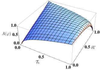
Figure 2: (Color online) $A(\varphi)$ as a function of ${\cal{T}}_{b}$ and $\delta\Gamma$ for $\varphi=\pi/2$. Refer to Eq. (49).

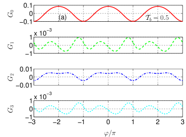
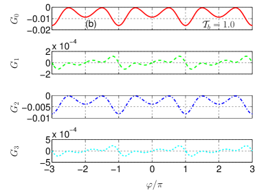
Figure 3: (Color online) Conductance coefficients as a function of $\varphi$. $G_{0}$ and $G_{2}$ are offset for simplicity. Parameters are $\Gamma_{0}=1$, $\delta\Gamma=0.2$, $\Gamma_{\alpha}=\Gamma_{0}(1\pm\delta\Gamma)$, $\varepsilon_{d}=-5\Gamma_{0}$, and $T=\Gamma_{0}$. Here, the conductance coefficients are scaled by $e^{n+2}/(2^{n-1}n!h)$.

V Kondo corrrelations

We can now go to next order in the equation-of-motion technique to describe the onset of Kondo correlations. Thus, we obtain the equations of motion for the three functions appearing on the right-hand side of Eq. (37), and approximate the new Green’s functions that appear in the procedure by making the decouplings, lac81

$$\langle\langle c_{\alpha k\sigma}c_{\beta r\bar{\sigma}}^{\dagger}d_{\bar{\sigma}},d_{\sigma}^{\dagger}\rangle\rangle \approx\langle c_{\beta r\bar{\sigma}}^{\dagger}d_{\bar{\sigma}}\rangle\langle\langle c_{\alpha k\sigma},d_{\sigma}^{\dagger}\rangle\rangle\,,$$ (55a)

$$\langle\langle c_{\alpha k\sigma}d_{\bar{\sigma}}^{\dagger}c_{\beta r\bar{\sigma}},d_{\sigma}^{\dagger}\rangle\rangle \approx\langle d_{\bar{\sigma}}^{\dagger}c_{\beta r\bar{\sigma}}\rangle\langle\langle c_{\alpha k\sigma},d_{\sigma}^{\dagger}\rangle\rangle\,,$$ (55b)

$$\langle\langle d_{\bar{\sigma}}^{\dagger}c_{\alpha k\bar{\sigma}}c_{\beta r\sigma},d_{\sigma}^{\dagger}\rangle\rangle \approx\langle d_{\bar{\sigma}}^{\dagger}c_{\alpha k\bar{\sigma}}\rangle\langle\langle c_{\beta r\sigma},d_{\sigma}^{\dagger}\rangle\rangle\,,$$ (55c)

$$\langle\langle c_{\beta r\bar{\sigma}}^{\dagger}c_{\alpha k\bar{\sigma}}d_{\sigma},d_{\sigma}^{\dagger}\rangle\rangle \approx\langle c_{\beta r\bar{\sigma}}^{\dagger}c_{\alpha k\bar{\sigma}}\rangle\langle\langle d_{\sigma},d_{\sigma}^{\dagger}\rangle\rangle\,,$$ (55d)

$$\langle\langle c_{\alpha k\bar{\sigma}}^{\dagger}c_{\beta r\bar{\sigma}}d_{\sigma},d_{\sigma}^{\dagger}\rangle\rangle \approx\langle c_{\alpha k\bar{\sigma}}^{\dagger}c_{\beta r\bar{\sigma}}\rangle\langle\langle d_{\sigma},d_{\sigma}^{\dagger}\rangle\rangle\,,$$ (55e)

$$\langle\langle c_{\alpha k\bar{\sigma}}^{\dagger}d_{\bar{\sigma}}c_{\beta r\sigma},d_{\sigma}^{\dagger}\rangle\rangle \approx\langle c_{\alpha k\bar{\sigma}}^{\dagger}d_{\bar{\sigma}}\rangle\langle\langle c_{\beta r\sigma},d_{\sigma}^{\dagger}\rangle\rangle\,.$$ (55f)

In what follows, we take the limit $U\to\infty$, in which case the term $\langle\langle c_{\alpha k\bar{\sigma}}^{\dagger}d_{\sigma}d_{\bar{\sigma}},d_{\sigma}^{\dagger}\rangle\rangle$ does not give any contribution. After little algebra, we find,

$$\langle\langle d_{\sigma},d_{\sigma}^{\dagger}\rangle\rangle^{r}=\frac{1-\langle n_{d\bar{\sigma}}\rangle-\delta n_{d\bar{\sigma}}(\omega)}{\omega+i0^{+}-\varepsilon_{d}-\left(1-\delta n_{d\bar{\sigma}}(\omega)\right)\Sigma_{0}(\omega)-\Sigma_{1}(\omega)}\,,$$ (56)

where

$$\delta n_{d\bar{\sigma}}(\omega)=-\frac{\widetilde{\Gamma}}{2\pi}\int d\omega^{\prime}~{}\frac{f_{peq}(\omega^{\prime})}{\omega^{\prime}-\omega-i0^{+}}\left[\langle\langle d_{\bar{\sigma}},d_{\bar{\sigma}}^{\dagger}\rangle\rangle_{\omega^{\prime}}^{r}\right]^{\ast}\,,$$ (57)

and

$$\Sigma_{0}(\omega) =-i\frac{\widetilde{\Gamma}}{2}-\frac{1}{4}\sqrt{\alpha{\cal{T}}_{b}}\Gamma\cos(\varphi)\,,$$ (58a)

$$\Sigma_{1}(\omega) =-\frac{\widetilde{\Gamma}}{2\pi}\int d\omega^{\prime}~{}\frac{f_{peq}(\omega^{\prime})}{\omega^{\prime}-\omega-i0^{+}}$$

$$\times\left\{1+\left[\Sigma_{0}(\omega^{\prime})\langle\langle d_{\bar{\sigma}},d_{\bar{\sigma}}^{\dagger}\rangle\rangle_{\omega^{\prime}}^{r}\right]^{\ast}\right\}\,.$$ (58b)

The derivation of this expression for the retarded Green function is explained in App. B.

To lowest order in $\Gamma$, Eq. (56) can be further simplified as

$$\langle\langle d_{\sigma},d_{\sigma}^{\dagger}\rangle\rangle=\frac{1-\langle n_{d\bar{\sigma}}\rangle}{\omega+i0^{+}-\varepsilon_{d}-\Sigma_{r}(\omega)}\,,$$ (59)

where

$$\Sigma_{r}(\omega)=\Sigma_{0}(\omega)+\Sigma_{1}(\omega)\,,$$ (60)

with

$$\Sigma_{1}(\omega)=-\frac{\widetilde{\Gamma}}{2\pi}\int d\omega^{\prime}~{}\frac{f_{peq}(\omega^{\prime})}{\omega^{\prime}-\omega-i0^{+}}\,.$$ (61)

Here, we note that for $\Gamma_{L}=\Gamma_{R}$ the self-energy obeys the following symmetry

$$\Sigma_{r}(\varphi,V)=\Sigma_{r}(-\varphi,-V)\,.$$ (62)

In turn, this property implies that the occupation and the conductance obey the even-odd symmetry also in the Kondo regime (at least when the coupling is not very strong).

Together with Eqs. (25) and (27) the Green function of Eq. (56) can be obtained from a self-consistent procedure. But before solving this system of equations using numerical methods, we briefly discuss two limits (high and low temperatures) to clarify the origin of magnetoasymmetries in the Kondo regime.

V.1 High-temperature regime

In this case, $\delta n_{d\bar{\sigma}}$ is a small correction and an expansion can be done. To first order in $\Gamma$ it can be shown that the position of the virtual level is renormalized to $\varepsilon_{d}^{\prime}$

$$\varepsilon_{d}^{\prime}=\varepsilon_{d}-\frac{1}{4}\sqrt{\alpha{\cal{T}}_{b}}\Gamma\cos(\varphi)-\frac{\widetilde{\Gamma}}{2\pi}\ln\frac{\sqrt{(\varepsilon_{d}^{\prime}-E_{F})^{2}+(\pi/\beta)^{2}}}{D}\,,$$ (63)

for $\beta(\omega-E_{F})\gg 1$. If $\beta|\varepsilon_{d}-E_{F}|\gg 1$ we have

$$\varepsilon_{d}^{\prime}=\varepsilon_{d}-\frac{1}{4}\sqrt{\alpha{\cal{T}}_{b}}\Gamma\cos(\varphi)-\frac{\widetilde{\Gamma}}{2\pi}\ln\frac{|\varepsilon_{d}^{\prime}-E_{F}|}{D}\,.$$ (64)

From the equation above, the Kondo temperature is given by

$$k_{B}T_{K}=D\exp\left[\frac{2\pi}{\widetilde{\Gamma}}\left(\varepsilon_{d}-\frac{1}{4}\sqrt{\alpha{\cal{T}}_{b}}\Gamma\cos(\varphi)\right)\right]\,.$$ (65)

The Kondo temperature marks the energy scale below which nontrivial spin fluctuations start to play a dominant role, leading to an antiferromagnetic exchange between the dot electron and the conduction electrons. We note that for a quantum dot inserted in an Aharonov-Bohm ring and in the presence of an applied flux, $T_{K}$ depends on $\xi$ and $\varphi$ but the dependence on the flux is weak.lop05 Furthermore, the Kondo temperature is a static quantity and, as such, is always a symmetric function of the flux.

We compare in Fig. 4 the value of $T_{K}$ with the Kondo temperature of a two-terminal quantum dot,

$$k_{B}T_{K}^{(0)}\sim D\exp\left\{\frac{2\pi\varepsilon_{d}}{\Gamma}\right\}\,,$$ (66)

and plot the ratio $T_{K}/T_{K}^{(0)}$ as a function of the direct channel tunneling probability [Fig. 4(a)] and the flux [Fig. 4(b)]. For $\varphi=0$ and ${\cal{T}}_{b}=0$ we recover $T_{K}=T_{K}^{(0)}$ as expected. As ${\cal{T}}_{b}$ increases for $\varphi=0$, the Kondo temperature decreases since electrons preferably travel along the upper arm. However, for fluxes above $\varphi=\pi/2$, the level renormalization due to $\cos\varphi$ is positive and the curve $T_{K}/T_{K}^{(0)}$ becomes nonmonotonous due to the competition between the renormalized dot level and broadening. This can be more clearly seen in Fig. 4(b).

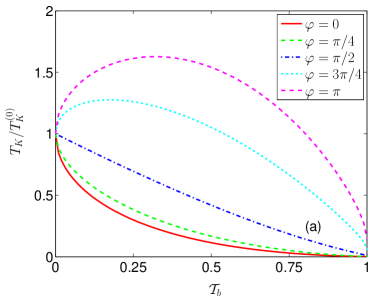
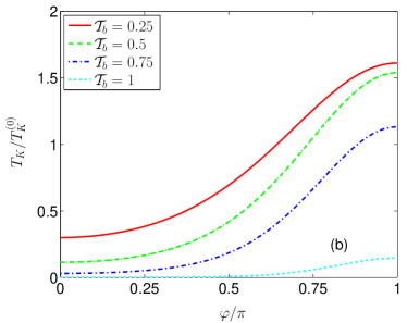
Figure 4: (Color online) Kondo temperature $T_{K}$ as a function of ${\cal{T}}_{b}$ and $\varphi$. The parameters are $D=1$, $\varepsilon_{d}=-0.05$, $U=\infty$, and $\Gamma_{L}=\Gamma_{R}=0.031$. For these parameters, $T_{K}^{(0)}\approx 0.0063$.

V.2 Low-temperature regime

At low-temperature $\delta n_{d\bar{\sigma}}$ must be large, especially near the Fermi level. If we suppose that ${\cal{G}}_{d\sigma,d\sigma}^{r}(\omega)$ varies smoothly near the Fermi level, Eq. (57) can be approximated as

$$\delta n_{d\bar{\sigma}}(\omega)\approx-\frac{\widetilde{\Gamma}}{2\pi}\left[{\cal{G}}_{d\sigma,d\sigma}^{r}\right]^{\ast}\left[\frac{i\pi}{2}+\ln\frac{2\pi}{\beta D}\right.\\ \left.+\Psi\left(\frac{1}{2}-i\beta\frac{(\omega-E_{F})}{2\pi}\right)\right]\,.$$ (67)

Inserting Eq. (67) into Eq. (56), we find

$${\cal{G}}_{d\sigma,d\sigma}^{r}(E_{F})=\frac{2}{\widetilde{\Gamma}}\sin(\theta)e^{-i\theta}\,.$$ (68)

Here, the value of $\theta$ is related to the number of $d$ electrons according to the Friedel-Langreth sum rule,Langreth

$$\theta=\frac{\pi\langle n_{d}\rangle}{2}\approx\frac{\pi}{2}\,.$$ (69)

This implies

$$\langle\langle d_{\sigma},d_{\sigma}^{\dagger}\rangle\rangle_{E_{F}}=\frac{1}{i\widetilde{\Gamma}/2}\,.$$ (70)

Then, the linear conductance can be written as

$$G^{(0)}(\varphi)=\frac{2e^{2}}{h}\alpha\left[1-{\cal{T}}_{b}\cos^{2}(\varphi)\right]\,.$$ (71)

This result is exact in the limit $k_{B}T,V\to 0$. For nonzero voltages, one should take into account that the imaginary part of the interaction self-energy of ${\cal{G}}_{d\sigma,d\sigma}^{r}$ depends on $V$ but this dependence is weak for $eV\ll k_{B}T_{K}$ and can be safely neglected. As a result, deep in the Kondo regime the conductance preserves the Onsager symmetry since in the Fermi liquid picture the Kondo resonance behaves as a noninteracting system with renormalized parameters. Charge fluctuations are quenched and transport becomes $B$-symmetric. This regime is beyond the scope of our method and we prefer not to present numerical results for very low temperatures. However, the expected scenario would be as follows: for very low temperatures the current would be $B$-symmetric and asymmetries would arise as temperature approaches $T_{K}^{(0)}$. In the opposite case, for temperatures much larger than $T_{K}^{(0)}$ transport is thermally assisted and the magnetoasymmetric effect also disappears.san05 Therefore, we expect a large magnetoasymmetry for temperatures of the order of $T_{K}^{(0)}$ for which charge fluctuations are large. We confirm this expectation in the numerical results reported below.

V.3 Numerical results

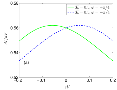
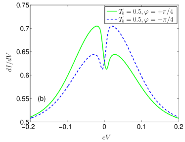
Figure 5: (Color online) Differential conductance $dI/dV$ ($2e^{2}/h$) as a function of the applied bias $eV$ for $D=1$, $\varepsilon_{d}=-0.05$, $U=\infty$, $\Gamma_{L}=\Gamma_{R}=0.031$, and $\varphi=\pi/4$. Temperatures are $T=10T_{K}^{(0)}$ (a) and $0.1T_{K}^{(0)}$ (b).

We numerically investigate the evolution of the magnetoasymmetry when temperature is lowered from the Coulomb blockade regime to the Kondo temperature. We first illustrate the generic behavior in Fig. 5, which shows the differential condutance $dI/dV$ a a function of the applied voltage $V$ for opposite orientations of the magnetic field. To compute the derivative of the current we have employed a numerical finite difference method.

In the top panel of Fig. 5, the temperature is large enough that Kondo correlations can be neglected. Then, the dot is in the Coulomb blockade regime and a small current is expected since the dot level is below the Fermi energy ($\varepsilon_{d}=-0.05$). However, the bridge channel is partially open and the system conductance reaches around $0.55\times 2e^{2}/h$ at $V=0$. This value is independent of the magnetic orientation, as expected. But when $V$ departs from equilibrium, the differential conductance behaves differently for $+\varphi$ and $-\varphi$. We recall that the effective position of the effective resonance depends on the charge state of the dot, as discussed in Sec. IV. Since the charge response of the system is not a symmetric function of $\varphi$, $dI/dV$ peaks at different voltages for opposite magnetic fields.

In Fig. 5(b) we depict $dI/dV$ in the low temperature case. We observe for both field orientations a dip around $V=0$. This dip is known to arise from the destructive interference between partial waves propagating through the upper arm and resonantly hopping across the dot.bul01 We emphasize that the dot bare level, $\varepsilon_{d}$, is the same for both calculations but in the Kondo regime transport is dominated by the narrow resonance formed at the Fermi level due to the higher-order tunneling processes that originate the Kondo effect. As a result, the Fano interference between the Kondo resonance and the background channel gives rise to the pronounced dip at zero bias. In our case, we obtain an asymmetric lineshape for the dip due to the magnetoasymmetric response of the dot away from equilibrium. As a consequence, the difference in $dI/dV$ for $+\varphi$ and $-\varphi$ is more visible in the Kondo regime, as can be seen in Fig. 5(b) compared to Fig. 5(a).

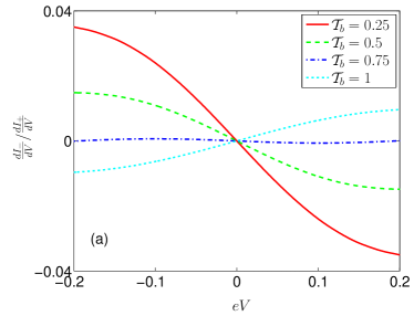
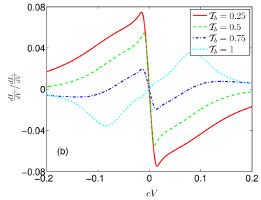
Figure 6: (Color online) Ratio of differential conductances $dI_{\pm}/dV$ ($2e^{2}/h$) as a function of the applied bias $eV$. Here, $dI_{\pm}/dV$ is defined as $d(I(\varphi)\pm I(-\varphi))/dV$. Parameters are $D=1$, $\varepsilon_{d}=-0.05$, $U=\infty$, $\Gamma_{L}=\Gamma_{R}=0.031$, and $\varphi=\pi/4$. Temperatures are $T=10T_{K}^{(0)}$ (a) and $0.1T_{K}^{(0)}$ (b).

We now define the symmetric ($+$) and antisymmetric parts ($-$) of $dI/dV$,

$$\frac{dI_{\pm}}{dV}=\frac{dI(\varphi)}{dV}\pm\frac{dI(-\varphi)}{dV}\,.$$ (72)

In Fig. 6 we plot the ratio between these two components as a function of the applied bias $V$ for a fixed value of the flux ($\varphi=\pi/4$) and for different values of the nonresonant transmission $\mathcal{T}_{b}$. In Fig 6(a) we set the temperature to a high value compared to the Kondo temperature. For $\mathcal{T}_{b}=0.5$ the magnetoasymmetry is always finite for $V\neq 0$. For voltages around zero, the magnetoasymmetry is a linear function of $V$ since the largest contribution stems from the $G_{1}$ coefficient in the current–voltage expansion. In the limit of high bias, the magnetoasymmetry saturates.san08 Interestingly, with increasing $\mathcal{T}_{b}$ the magnetoasymmetry is reduced and changes sign for a fixed $V$. Thefore, the sign of the asymmetry can be tuned with the background transmission of the nonresonant channel. The situation is similar to the magnetoasymmetry of a two-terminal quantum dot when transport is dominated by elastic cotunneling processes.san05 In that case, the sign of the asymmetry can be changed with the gate voltage which moves the dot level position above and below the particle-hole symmetric point.san05 In our case, $\mathcal{T}_{b}$ acts as an effective gate which changes the position of the level since $\varepsilon_{0}$ is renormalized according to Eq. (22).

When temperature is lowered, we observe that the transition from positive to negative asymmetries as $V$ is tuned, is rather abrupt, see Fig 6(b). We note that as voltage approaches $V=0$ one sweeps along the strongly asymmetric dip structure found in Fig 5(b), for which the difference between the cases $+\varphi$ and $-\varphi$ is most clear. Then, it is the Kondo resonance that produces the abrupt change in the magnetoasymmetry profile as compared to the high temperature case [Fig 6(a)]. As a consequence, Kondo correlations enhance the deviations from the Onsager symmetry since the narrow resonance is more sensitive to changes in the orientation of the magnetic field.zeeman For instance, we observe in Fig 6(b) a revival of the magnetoasymmetry for $\mathcal{T}_{b}=0.75$, which almost vanished in the high temperature case. However, if temperature is further lowered ($T\ll T_{K}^{(0)}$) for $\varepsilon_{d}\ll E_{F}$, charge fluctuations would be quenched and the Kondo resonance would be pinned at the Fermi level, independently of $\varphi$ and $\mathcal{T}_{b}$. As a consequence, the magnetoasymmetry would tend to vanish.

VI Shot noise

The shot noise is a valuable tool in the characterization of the transport properties of mesoscopic systems.bla00 For systems described with Anderson impurity models like ours, the electron repulsion term $U$ introduces correlations which can be investigated through the noise. Then, the problem becomes involved, although the effect of Kondo correlations in the shot noise have been already addressed in a number of papers.her92 ; yam94 ; din97 ; mei02 ; don02 ; avi03 ; aon03 ; lop03a ; lop03b ; san05b ; wu05 ; gol06 ; sel06 ; zha07 ; zar07 .

Magnetoasymmetries in noise have recently attracted a good deal of attention due to the (weakly) nonequilibrium relations between the asymmetries of the current and that of the noise to leading order in a voltage expansion.foe08 ; sai08 ; san09 ; uts09 The subject is also of interest because it poses questions about the validity of fluctuation theorems out of equilibrium.foe08 In this section our goal is to calculate the noise power for our system in the limits of both weak and strong electron-electron interactions and check the nonequilibrium fluctuation relations.

The current noise between terminals $\alpha$ and $\beta$ is defined as

$$S_{\alpha\beta}(t-t^{\prime})=\frac{1}{2}\left\{\langle[\hat{I}_{\alpha}(t),\hat{I}_{\beta}(t^{\prime})]_{+}\rangle-2\langle\hat{I}_{\alpha}\rangle\langle\hat{I}_{\beta}\rangle\right\}\,,$$ (73)

where $\hat{I}$ represents a current operator. The Fourier transformation of the current noise (the noise power) reads

$$S(\omega)\equiv\int_{-\infty}^{\infty}dt~{}e^{i\omega t}S(t)\,.$$ (74)

where we have defined the Fourier transform without the prefactor $2$. In the following, we present results for the zero frequency case [the shot noise $S\equiv S(0)$].

The noise definition of Eq. (73) contains correlations between currents that, quite generally, involve four operators. To treat the resulting two-body Green’s functions, we make use of cluster expansion,lop03a ; san05b ; zha07

$$\langle\hat{O}_{\mu\sigma}^{\dagger}\hat{O}_{\nu\sigma}\hat{O}_{\mu^{\prime}\sigma^{\prime}}^{\dagger}\hat{O}_{\nu^{\prime}\sigma^{\prime}}\rangle\approx\langle\hat{O}_{\mu\sigma}^{\dagger}\hat{O}_{\nu\sigma}\rangle\langle\hat{O}_{\mu^{\prime}\sigma^{\prime}}^{\dagger}\hat{O}_{\nu^{\prime}\sigma^{\prime}}\rangle\\ +\delta_{\sigma\sigma^{\prime}}\langle\hat{O}_{\mu\sigma}^{\dagger}\hat{O}_{\nu^{\prime}\sigma^{\prime}}\rangle\langle\hat{O}_{\nu\sigma}\hat{O}_{\mu^{\prime}\sigma^{\prime}}^{\dagger}\rangle$$ (75)

which amounts to neglecting two-body connected Green’s functions. As a result, the shot noise is expressed in terms of one-body Green’s functions. This is a strong assumption that can lead to deviations from well known relations. Nevertheless, interactions are included (at the level of the Lacroix’s approximation). The calculation is lengthy and we refer the reader to App. C. Here, we consider limit cases only.

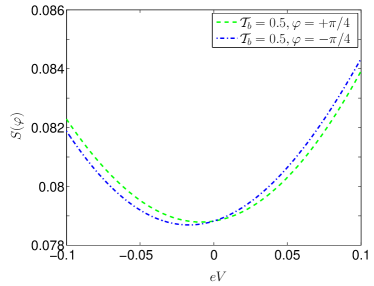
Figure 7: (Color online) Noise ($2e^{2}/h$) as a function of voltage for two opposite orientations of $\varphi$. Parameters are $D=1$, $\varepsilon_{d}=-0.05$, $U=\infty$, and $\Gamma_{L}=\Gamma_{R}=0.031$.

For the noninteracting case and at zero temperature we recover the known expression,

$$S=\frac{e^{2}}{h}\sum_{\sigma}\int_{-eV/2}^{eV/2}d\varepsilon~{}{\cal{T}}_{\sigma}(\omega)\left[1-{\cal{T}}_{\sigma}(\omega)\right]\,,$$ (76)

where the transmission is given by Eq. (18). As expected, the noise is an even function of $\varphi$ to all orders in $V$. However, interactions destroy this symmetry already in the linear regime of the noise response. In Fig. 7 we show the noise as a function of $V$ in the strongly interacting case. We can observe that the slope of the noise curves at $V=0$ differ for opposite field orientations. Another interesting feature is that for some voltages the nonequilibrium noise can be reduced from its equilibrium value.for09

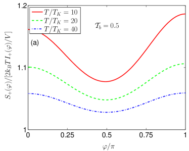
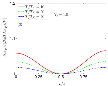
Figure 8: (Color online) Identification of the fluctuations-dissipation theorem as a function of $\varphi$. Parameters are $D=1$, $\varepsilon_{d}=-0.05$, $U=\infty$, and $\Gamma_{L}=\Gamma_{R}=0.031$. The applied bias is $eV=0.01T_{K}^{(0)}$.

To gain further insight, we expand the noise in powers of $V$,

$$S=S_{0}+S_{1}V+\ldots\,.$$ (77)

$S_{0}$ is the equilibrium noise describing thermal fluctuations. Since these fluctuations do not distinguish between $+\varphi$ and $-\varphi$, $S_{0}$ is an even function of the magnetic field. An alternate proof of this statement is based on the equilibrium fluctuation-dissipation theorem, which relates $S_{0}$ to the linear conductance $G_{0}$,

$$S_{0}=2k_{B}TG_{0}\,.$$ (78)

Since for $G_{0}$ the Onsager symmetry holds, $S_{0}$ should be even for a two-terminal setup.

We now show the numerical results of our model for different temperatures. We define the symmetric and antisymmetric components of the noise and the current as before,

$$S_{\pm} =S(+\varphi)\pm S(-\varphi)\,,$$ (79a)

$$I_{\pm} =I(+\varphi)\pm I(-\varphi)\,.$$ (79b)

We consider symmetric couplings. As result, the even-odd properties of the transport coefficients allow us to write,

$$\frac{S_{+}}{I_{+}/V} =2k_{B}T\,$$ (80a)

$$\frac{S_{-}}{I_{-}/V^{2}} =2k_{B}T\,.$$ (80b)

Corrections to these relations are of order $V^{2}$ and can be neglected for $eV\ll k_{B}T$. The first relation is merely a restatement of Eq. (78). The second relation is a nonequilibrium relation that connect the magnetoasymmetries corresponding to both the linear-response noise ($S_{1}$) and the leading-order nonlinear conductance ($G_{1}$).

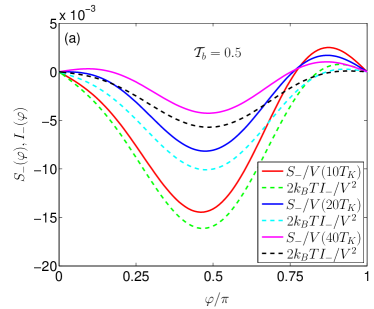
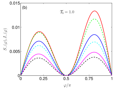
Figure 9: (Color online) Antisymmetric parts of noise, $S_{-}(\varphi)$, and current, $I_{-}(\varphi)$, as a function of $\varphi$. Parameters are $D=1$, $\varepsilon_{d}=-0.05$, $U=\infty$, and $\Gamma_{L}=\Gamma_{R}=0.031$. The applied bias is $eV=0.01T_{K}^{(0)}$.

We take a small voltage ($V=0.01T_{K}^{(0)}/e$) and plot in Fig. 8 the relation given by Eq. (80a) as a function of the flux for two different values of the background transmission. In bot cases we find that Eq. (80a) is approximately fulfilled with small deviations which we attribute to the assumption of Eq. (75). We note that deviations grow for smaller temperatures since in this case the Kondo correlations become more relevant and our model for the noise starts to break down. When the nonresonant channel is fully open (bottom panel of Fig. 8), the deviations are less important since electrons preferably travel along the upper arm and consequently feel less the intradot interactions.

The validity of the nonequilibrium fluctuation relation [Eq. (80b)] is analyzed in Fig. 9. Here we plot separately the two terms of Eq. (80b). We find a strong ressemblance between $S_{1}$ and $G_{1}$ for all magnetic fields. Deviations also exist as in the calculation of the symmetric components but they fulfill the same pattern, namely, they tend to disappear when the background transmission is close to 1 and the temperature increases well above the Kondo temperature. Although our results are not a conclusive proof of Eq. (80b) for strongly interacting systems, the errors are small and compatible with the same deviations found in the equilibrium case (Fig. 8).

VII Conclusions

We have shown that the current–voltage characteristics of a two-terminal quantum-dot mesoscopic interferometer is not an even function of the applied flux in the nonlinear regime of transport and when intradot interactions are taken into account. The interference pattern of the ring at a finite bias is thus not symmetric under reversal of the magnetic field. We have carefully investigated the symmetry properties of the conductance coefficients in a current–voltage expansion. Our discussions are based on the properties of the charge response of the dot when a finite bias is applied to the system. When the quantum dot is in the Coulomb-blockade regime, we find for most cases that the even coefficients are symmetric functions of the field while the odd coefficients does not show any relevant symmetry in the general case. Only when the dot is symmetrically coupled to the leads the odd coefficients are antisymmetric.

We have also calculated the magnetoasymmetry of the system in the strong coupling regime, when the dot is described with Kondo correlations. In this case, the magnetoasymmetry shows an abrupt transition between positive and negative values when the voltage crosses the Fermi energy. As a result, the Kondo resonance dominates the magnetoasymmetry lineshape when the voltage is of the order of the Kondo temperature. A further extension of this work could be focused on the very low temperature regime using, e.g., slave-boson techniques.

Finally, we have investigated the asymmetry in the shot noise, finding a correlation between the noise and the current magnetoasymmetry to leading order in the applied voltage. This nonequilibrium fluctuation relation seems to apply in a wide range of parameters (temperature, direct channel transmission and applied fluxes). However, further work is needed to reduce the deviations which are most probably due to our approximations. In particular, it would be interesting to analyze the role of the third cumulant of the current (or better the entire full counting statistics) under field reversal.

Appendix A Lesser Green’s Function of the Dot

In general, the lesser Green’s function for an interacting dot cannot be obtained from the equation of motion technique without introducing additional assumptions. Following Ng’s heuristic approach, here we employ an ansatz for interacting lesser and greater Green’s functions Ng96 . Using the lesser and greater self-energies for a noninteracting dot

$$\Sigma_{\sigma}^{<(0)}(\omega) =+i\sum_{\alpha}\bar{\Gamma}_{\alpha}f_{\alpha}(\omega)\,,$$ (81a)

$$\Sigma_{\sigma}^{>(0)}(\omega) =-i\sum_{\alpha}\bar{\Gamma}_{\alpha}\left[1-f_{\alpha}(\omega)\right]\,,$$ (81b)

with

$$\bar{\Gamma}_{L} =\frac{1}{(1+\xi)^{2}}\left(\Gamma_{L}+\xi\Gamma_{R}\right)+\frac{\widetilde{\Gamma}}{2}\sqrt{\alpha{\cal{T}}_{b}}\sin(\varphi)\,,$$ (82a)

$$\bar{\Gamma}_{R} =\frac{1}{(1+\xi)^{2}}\left(\Gamma_{R}+\xi\Gamma_{L}\right)-\frac{\widetilde{\Gamma}}{2}\sqrt{\alpha{\cal{T}}_{b}}\sin(\varphi)\,.$$ (82b)

we assume that lesser and greater Green’s functions for an interacting dot can be written in the form

$$\Sigma_{\sigma}^{<}(\omega) =+i\sum_{\alpha}\bar{\Gamma}_{\alpha}f_{\alpha}R_{\sigma}(\omega)\,,$$ (83a)

$$\Sigma_{\sigma}^{>}(\omega) =-i\sum_{\alpha}\bar{\Gamma}_{\alpha}\left[1-f_{\alpha}\right]R_{\sigma}(\omega)\,.$$ (83b)

The explicit form of $R_{\sigma}(\omega)$ can be obtained from the relation

$$\Sigma_{\sigma}^{>}(\omega)-\Sigma_{\sigma}^{<}(\omega)=\Sigma_{\sigma}^{r}(\omega)-\Sigma_{\sigma}^{a}(\omega)\,.$$ (84)

Employing the identity,

$${\cal{G}}_{d\sigma,d\sigma}^{>}(\omega)-{\cal{G}}_{d\sigma,d\sigma}^{<}(\omega)={\cal{G}}_{d\sigma,d\sigma}^{r}(\omega)-{\cal{G}}_{d\sigma,d\sigma}^{a}(\omega)\,,$$ (85)

it finally yields

$${\cal{G}}_{d\sigma,d\sigma}^{<}(\omega)=-f_{peq}(\omega)\left[{\cal{G}}_{d\sigma,d\sigma}^{r}(\omega)-{\cal{G}}_{d\sigma,d\sigma}^{a}(\omega)\right]\,,$$ (86)

with

$$f_{peq}(\omega)=\frac{\sum_{\alpha}\bar{\Gamma}_{\alpha}f_{\alpha}(\omega)}{\sum_{\alpha}\bar{\Gamma}_{\alpha}}\,.$$ (87)

Appendix B Evaluation of expectation values

In deriving Eq. (56), we have to evaluate the expectation values $\langle d_{\bar{\sigma}}^{\dagger}c_{\alpha k\bar{\sigma}}\rangle$ and $\sum_{\beta,r}V_{\beta}\langle c_{\beta r\bar{\sigma}}^{\dagger}c_{\alpha k\bar{\sigma}}\rangle$. First, let us concentrate on $\langle d_{\bar{\sigma}}^{\dagger}c_{\alpha k\bar{\sigma}}\rangle$. In equilibirum, the quantities can be calculated by using the fluctuation-dissipation theorem,

$$\langle d_{\bar{\sigma}}^{\dagger}c_{\alpha k\bar{\sigma}}\rangle=-\frac{1}{\pi}\int d\omega~{}f_{eq}(\omega)\operatorname{Im}\left[\langle\langle c_{\alpha k\bar{\sigma}},d_{\bar{\sigma}}^{\dagger}\rangle\rangle_{\omega}^{r}\right]\,.$$ (88)

However, the fluctuation-dissipation theorem cannot be employed in nonequilibrium. Then, in general,

$$\langle d_{\bar{\sigma}}^{\dagger}c_{\alpha k\bar{\sigma}}\rangle=\frac{1}{2\pi i}\int d\omega~{}\langle\langle c_{\alpha k\bar{\sigma}},d_{\bar{\sigma}}^{\dagger}\rangle\rangle_{\omega}^{<}\,.$$ (89)

Note that $\langle\langle c_{\alpha k\bar{\sigma}},d_{\bar{\sigma}}^{\dagger}\rangle\rangle_{\omega}^{<}$ cannot be obtained exactly becuase of the dot lesser Green’s function. Here, we thus assume the following pseudoequilibrium form

$$\langle\langle c_{\alpha k\bar{\sigma}},d_{\bar{\sigma}}^{\dagger}\rangle\rangle_{\omega}^{<}=-f_{peq}(\omega)\left(\langle\langle c_{\alpha k\bar{\sigma}},d_{\bar{\sigma}}^{\dagger}\rangle\rangle_{\omega}^{r}-\langle\langle c_{\alpha k\bar{\sigma}},d_{\bar{\sigma}}^{\dagger}\rangle\rangle_{\omega}^{a}\right)\,.$$ (90)

Then, we have

$$\langle d_{\bar{\sigma}}^{\dagger}c_{\alpha k\bar{\sigma}}\rangle=\\ -\frac{1}{2\pi i}\int d\omega~{}f_{peq}(\omega)\left(\langle\langle c_{\alpha k\bar{\sigma}},d_{\bar{\sigma}}^{\dagger}\rangle\rangle_{\omega}^{r}(\varphi)-\langle\langle c_{\alpha k\bar{\sigma}},d_{\bar{\sigma}}^{\dagger}\rangle\rangle_{\omega}^{a}(\varphi)\right)\,,$$ (91)

where

$$\langle\langle c_{Lk\bar{\sigma}},d_{\bar{\sigma}}^{\dagger}\rangle\rangle_{\omega}^{r} =\frac{g_{Lp\bar{\sigma}}^{r}}{1+\xi}\left(V_{L}-i\sqrt{\xi}e^{-i\varphi}V_{R}\right)\langle\langle d_{\bar{\sigma}},d_{\bar{\sigma}}^{\dagger}\rangle\rangle_{\omega}^{r}\,,$$ (92a)

$$\langle\langle c_{Rk\bar{\sigma}},d_{\bar{\sigma}}^{\dagger}\rangle\rangle_{\omega}^{r} =\frac{g_{Rq\bar{\sigma}}^{r}}{1+\xi}\left(V_{R}-i\sqrt{\xi}e^{+i\varphi}V_{L}\right)\langle\langle d_{\bar{\sigma}},d_{\bar{\sigma}}^{\dagger}\rangle\rangle_{\omega}^{r}\,,$$ (92b)

and

$$\langle\langle c_{Lp\bar{\sigma}},d_{\bar{\sigma}}^{\dagger}\rangle\rangle_{\omega}^{a} =\frac{g_{Lp\bar{\sigma}}^{a}}{1+\xi}\left(V_{L}+i\sqrt{\xi}e^{-i\varphi}V_{R}\right)\langle\langle d_{\bar{\sigma}},d_{\bar{\sigma}}^{\dagger}\rangle\rangle_{\omega}^{a}\,,$$ (93a)

$$\langle\langle c_{Rq\bar{\sigma}},d_{\bar{\sigma}}^{\dagger}\rangle\rangle_{\omega}^{a} =\frac{g_{Rq\bar{\sigma}}^{a}}{1+\xi}\left(V_{R}+i\sqrt{\xi}e^{+i\varphi}V_{L}\right)\langle\langle d_{\bar{\sigma}},d_{\bar{\sigma}}^{\dagger}\rangle\rangle_{\omega}^{a}\,,$$ (93b)

with $g_{\alpha k\bar{\sigma}}^{r,a}=1/(\omega\pm i0^{+}-\varepsilon_{\alpha k\bar{\sigma}})$. Due to the approximations, however, the retarded Green’s function is not the complex conjugate of the advanced one so that this equation gives an unphysical result. To resolve this difficulty, we thus replace the quantity in the parenthesis by the time-reversal pair. That is,

$$\langle d_{\bar{\sigma}}^{\dagger}c_{\alpha k\bar{\sigma}}\rangle=-\frac{1}{2\pi i}\int d\omega~{}f_{peq}(\omega)\\ \times\left(\langle\langle c_{\alpha k\bar{\sigma}},d_{\bar{\sigma}}^{\dagger}\rangle\rangle_{\omega}^{r}(-\varphi)-\langle\langle c_{\alpha k\bar{\sigma}},d_{\bar{\sigma}}^{\dagger}\rangle\rangle_{\omega}^{a}(\varphi)\right)\,.$$ (94)

This yields a real expectation value as should be. Using Eq. (94), we thus have

$$\sum_{k}\frac{\langle d_{\bar{\sigma}}^{\dagger}c_{Lk\bar{\sigma}}\rangle}{\omega+i0^{+}-\varepsilon_{Lk\bar{\sigma}}}=-\frac{\rho_{0}}{1+\xi}\int d\omega^{\prime}~{}\frac{f_{peq}(\omega^{\prime})}{\omega^{\prime}-\omega-i0^{+}}\\ \times\left(V_{L}+i\sqrt{\xi}e^{-i\varphi}V_{R}\right)\left[\langle\langle d_{\bar{\sigma}},d_{\bar{\sigma}}^{\dagger}\rangle\rangle_{\omega^{\prime}}^{r}\right]^{\ast}\,,$$ (95a)

$$\sum_{k}\frac{\langle d_{\bar{\sigma}}^{\dagger}c_{Rk\bar{\sigma}}\rangle}{\omega+i0^{+}-\varepsilon_{Rk\bar{\sigma}}}=-\frac{\rho_{0}}{1+\xi}\int d\omega^{\prime}~{}\frac{f_{peq}(\omega^{\prime})}{\omega^{\prime}-\omega-i0^{+}}\\ \times\left(V_{R}+i\sqrt{\xi}e^{+i\varphi}V_{L}\right)\left[\langle\langle d_{\bar{\sigma}},d_{\bar{\sigma}}^{\dagger}\rangle\rangle_{\omega^{\prime}}^{r}\right]^{\ast}\,.$$ (95b)

In the same way:

$$\sum_{\beta,r,k}\frac{\langle c_{\beta r\bar{\sigma}}^{\dagger}c_{Lk\bar{\sigma}}\rangle}{\omega+i0^{+}-\varepsilon_{Lk\bar{\sigma}}}=-\frac{\rho_{0}}{1+\xi}\int d\omega^{\prime}~{}\frac{f_{peq}(\omega^{\prime})}{\omega^{\prime}-\omega-i0^{+}}\\ \times\left(V_{L}+i\sqrt{\xi}e^{-i\varphi}V_{R}\right)\left\{1+\left[\Sigma_{0}(\omega^{\prime})\langle\langle d_{\bar{\sigma}},d_{\bar{\sigma}}^{\dagger}\rangle\rangle_{\omega^{\prime}}^{r}\right]^{\ast}\right\}\,,$$ (96a)

$$\sum_{\beta,r,k}\frac{\langle c_{\beta r\bar{\sigma}}^{\dagger}c_{Rk\bar{\sigma}}\rangle}{\omega+i0^{+}-\varepsilon_{Rk\bar{\sigma}}}=-\frac{\rho_{0}}{1+\xi}\int d\omega^{\prime}~{}\frac{f_{peq}(\omega^{\prime})}{\omega^{\prime}-\omega-i0^{+}}\\ \times\left(V_{R}+i\sqrt{\xi}e^{+i\varphi}V_{L}\right)\left\{1+\left[\Sigma_{0}(\omega^{\prime})\langle\langle d_{\bar{\sigma}},d_{\bar{\sigma}}^{\dagger}\rangle\rangle_{\omega^{\prime}}^{r}\right]^{\ast}\right\}\,.$$ (96b)

Appendix C Expression of the shot noise

The current noise is defined as

$$S_{\alpha\beta}(t-t^{\prime})=\frac{1}{2}\left\{\langle[\hat{I}_{\alpha}(t),\hat{I}_{\beta}(t^{\prime})]_{+}\rangle-2\langle\hat{I}_{\alpha}\rangle\langle\hat{I}_{\beta}\rangle\right\}\,.$$ (97)

The current operator can be calculated from the time evolution of the occupation number operator

$$\hat{I}_{R}=\frac{ie}{\hbar}\left\{\sum_{p\in L,q\in R,\sigma}\left[We^{i\varphi}c_{Rq\sigma}^{\dagger}c_{Lp\sigma}-We^{-i\varphi}c_{Lp\sigma}^{\dagger}c_{Rq\sigma}\right]\right.\\ \left.+\sum_{q\in R,\sigma}\left[V_{R}c_{Rq\sigma}^{\dagger}d_{\sigma}-V_{R}^{\ast}d_{\sigma}^{\dagger}c_{Rq\sigma}\right]\right\}\,.$$ (98)

The current can be then obtained by taking the average of $\hat{I}_{R}$. Using the Keldysh Green’s functions, the current can be expressed as

$$\langle\hat{I}_{R}(t)\rangle=\frac{e}{h}\left[\sum_{p\in L,q\in R,\sigma}\left(We^{i\varphi}{\cal{G}}_{Lp\sigma,Rq\sigma}^{<}(t,t)\right.\right.\\ \left.\left.-We^{-i\varphi}{\cal{G}}_{Rq\sigma,Lp\sigma}^{<}(t,t)\right)\right.\\ \left.+\sum_{q\in R,\sigma}\left(V_{R}{\cal{G}}_{d\sigma,Rq\sigma}^{<}(t,t)-V_{R}^{\ast}{\cal{G}}_{Rq\sigma,d\sigma}^{<}(t,t)\right)\right]\,.$$ (99)

The Fourier transformation of the current noise is

$$S(\omega)\equiv\int_{-\infty}^{\infty}dt~{}e^{i\omega t}S(t)\,.$$ (100)

The zero-frequency noise power $S\equiv S(0)$ is referred to as shot noise. In the derivation, we make use of cluster expansion to treat two-body Green’s functions:lop03a ; san05b ; zha07

$$\langle\hat{O}_{\mu\sigma}^{\dagger}\hat{O}_{\nu\sigma}\hat{O}_{\mu^{\prime}\sigma^{\prime}}^{\dagger}\hat{O}_{\nu^{\prime}\sigma^{\prime}}\rangle\approx\langle\hat{O}_{\mu\sigma}^{\dagger}\hat{O}_{\nu\sigma}\rangle\langle\hat{O}_{\mu^{\prime}\sigma^{\prime}}^{\dagger}\hat{O}_{\nu^{\prime}\sigma^{\prime}}\rangle\\ +\delta_{\sigma\sigma^{\prime}}\langle\hat{O}_{\mu\sigma}^{\dagger}\hat{O}_{\nu^{\prime}\sigma^{\prime}}\rangle\langle\hat{O}_{\nu\sigma}\hat{O}_{\mu^{\prime}\sigma^{\prime}}^{\dagger}\rangle$$ (101)

In the frequency domain, using Eqs. (98) and (99) and cluster expansion the shot noise is given by

$$S=\frac{1}{2\pi}\frac{2(ie)^{2}}{\hbar}\int d\omega~{}\left\{W^{2}\left[e^{+2i\varphi}{\cal{G}}_{Lp^{\prime}\sigma,Rq\sigma}^{<}(\omega){\cal{G}}_{Lp\sigma,Rq^{\prime}\sigma}^{>}(\omega)+e^{-2i\varphi}{\cal{G}}_{Rq^{\prime}\sigma,Lp\sigma}^{<}(\omega){\cal{G}}_{Rq\sigma,Lp^{\prime}\sigma}^{>}(\omega)\right]\right.\\ -W^{2}\left[{\cal{G}}_{Rq^{\prime}\sigma,Rq\sigma}^{<}(\omega){\cal{G}}_{Lp\sigma,Lp^{\prime}\sigma}^{>}(\omega)+{\cal{G}}_{Lp^{\prime}\sigma,Lp\sigma}^{<}(\omega){\cal{G}}_{Rq\sigma,Rq^{\prime}\sigma}^{>}(\omega)\right]\\ +W\left[V_{R}e^{+i\varphi}{\cal{G}}_{d\sigma,Rq\sigma}^{<}(\omega){\cal{G}}_{Lp\sigma,Rq^{\prime}\sigma}^{>}(\omega)+V_{R}^{\ast}e^{-i\varphi}{\cal{G}}_{Rq^{\prime}\sigma,d\sigma}^{<}(\omega){\cal{G}}_{Rq\sigma,Lp^{\prime}\sigma}^{>}(\omega)\right]\\ -W\left[V_{R}e^{-i\varphi}{\cal{G}}_{d\sigma,Lp\sigma}^{<}(\omega){\cal{G}}_{Rq\sigma,Rq^{\prime}\sigma}^{>}(\omega)+V_{R}^{\ast}e^{+i\varphi}{\cal{G}}_{Lp^{\prime}\sigma,d\sigma}^{<}(\omega){\cal{G}}_{Rq\sigma,Rq^{\prime}\sigma}^{>}(\omega)\right]\\ -W\left[V_{R}^{\ast}e^{+i\varphi}{\cal{G}}_{Rq^{\prime}\sigma,Rq\sigma}^{<}(\omega){\cal{G}}_{Lp\sigma,d\sigma}^{>}(\omega)+V_{R}e^{-i\varphi}{\cal{G}}_{Rq^{\prime}\sigma,Rq\sigma}^{<}(\omega){\cal{G}}_{d\sigma,Lp^{\prime}\sigma}^{>}(\omega)\right]\\ +W\left[V_{R}^{\ast}e^{-i\varphi}{\cal{G}}_{Rq^{\prime}\sigma,Lp\sigma}^{<}(\omega){\cal{G}}_{Rq\sigma,d\sigma}^{>}(\omega)+V_{R}e^{+i\varphi}{\cal{G}}_{Lp^{\prime}\sigma,Rq\sigma}^{<}(\omega){\cal{G}}_{d\sigma,Rq^{\prime}\sigma}^{>}(\omega)\right]\\ +\left[V_{R}V_{R}{\cal{G}}_{d\sigma,Rq\sigma}^{<}(\omega){\cal{G}}_{d\sigma,Rq^{\prime}\sigma}^{>}(\omega)+V_{R}^{\ast}V_{R}^{\ast}{\cal{G}}_{Rq^{\prime}\sigma,d\sigma}^{<}(\omega){\cal{G}}_{Rq\sigma,d\sigma}^{>}(\omega)\right]\\ \left.-V_{R}V_{R}^{\ast}\left[{\cal{G}}_{Rq^{\prime}\sigma,Rq\sigma}^{<}(\omega){\cal{G}}_{d\sigma,d\sigma}^{>}(\omega)+{\cal{G}}_{d\sigma,d\sigma}^{<}(\omega){\cal{G}}_{Rq\sigma,Rq^{\prime}\sigma}^{>}(\omega)\right]\right\}\,,$$ (102)

where summations over momentum indices are assumed. Here, the Keldysh Green’s functions which appear on the r.h.s. of Eq. (102) can be expressed in terms of the dot Green’s functions, ${\cal{G}}_{d\sigma,d\sigma}^{<}(\omega)$ and ${\cal{G}}_{d\sigma,d\sigma}^{r,a}(\omega)$.

References

- (1) L. Onsager, Phys. Rev. 38, 2265 (1931).
- (2) H.B.G. Casimir, Rev. Mod. Phys. 17, 343 (1945).
- (3) M. Büttiker, Phys. Rev. Lett. 57, 1761 (1986).
- (4) A. Yacoby, M. Heiblum, D. Mahalu, and H. Shtrikman, Phys. Rev. Lett. 74, 4047 (1995).
- (5) A. Levy Yeyati and M. Büttiker, Phys. Rev. B 52, R14360 (1995).
- (6) G. Hackenbroich and H.A. Weidenmüller, Phys. Rev. Lett. 76, 110 (1996).
- (7) C. Bruder, R. Fazio and H. Schoeller, Phys. Rev. Lett. 76, 114 (1996).
- (8) A. Yacoby, R. Schuster and M. Heiblum, Phys. Rev. B 53, 9583 (1996).
- (9) R. Schuster, E. Buks, M. Heiblum, D. Mahalu, V. Umansky and H. Shtrikman, Nature 385, 417 (1997).
- (10) D. Sánchez and M. Büttiker, Phys. Rev. Lett. 93, 106802 (2004).
- (11) B. Spivak and A. Zyuzin, Phys. Rev. Lett. 93, 226801 (2004).
- (12) M. Büttiker and D. Sánchez, Int. J. Quantum Chem. 105, 906 (2005).
- (13) D. Sánchez and M. Büttiker, Phys. Rev. B 72, 201308 (2005).
- (14) M.L. Polianski and M. Büttiker, Phys. Rev. Lett. 96, 156804 (2006).
- (15) A. De Martino, R. Egger, and A. M. Tsvelik, Phys. Rev. Lett. 97, 076402 (2006).
- (16) A.V. Andreev and L.I. Glazman, Phys. Rev. Lett. 97, 266806 (2006).
- (17) M.L. Polianski and M. Büttiker, Phys. Rev. B 76, 205308 (2007).
- (18) D. Sánchez and K. Kang, Phys. Rev. Lett. 100, 036806 (2008).
- (19) R. Kalina, B. Szafran, S. Bednarek, and F.M. Peeters, Phys. Rev. Lett. 102 066807 (2009).
- (20) B. Szafran, M. R. Poniedzialek, and F.M. Peeters, Europhys. Lett. 87, 47002 (2009).
- (21) A.R. Hernández and C.H. Lewenkopf, Phys. Rev. Lett. 103 166801 (2009).
- (22) G.L.J.A. Rikken and P. Wyder, Phys. Rev. Lett. 94, 016601 (2005).
- (23) J. Wei, M. Schimogawa, Z. Whang, I. Radu, R. Dormaier, and D.H. Cobden, Phys. Rev. Lett. 95, 256601 (2005).
- (24) C. A. Marlow, R.P. Taylor, M. Fairbanks, I. Shorubalko, and H. Linke, Phys. Rev. Lett. 96, 116801 (2006).
- (25) R. Leturcq, D. Sánchez, G. Götz, T. Ihn, K. Ensslin, D.C. Driscoll, and A.C. Gossard, Phys. Rev. Lett. 96, 126801 (2006).
- (26) D. M. Zumbühl, C.M. Marcus, M.P. Hanson, and A.C. Gossard, Phys. Rev. Lett. 96, 206802 (2006).
- (27) L. Angers, E. Zakka-Bajjanni, R. Deblock, S. Guéron, H. Bouchiat, A. Cavanna, U. Gennser, and M. Polianksi, Phys. Rev. B 75, 115309 (2007).
- (28) D. Hartmann, L. Worschech, and A. Forchel, Phys. Rev. B 78, 113306 (2008).
- (29) A.D. Chepelianskii and H. Bouchiat, Phys. Rev. Lett. 102, 086810 (2009).
- (30) B. Brandenstein-Köth, L. Worschech, and A. Forchel, Appl. Phys. Lett. 95, 062106 (2009).
- (31) L. I. Glazman and M. E. Raikh, Pis’ma Zh. Éksp. Teor. Fiz. 47, 378 (1988) [JETP Lett. 47, 452 (1988)]; T. K. Ng and P. A. Lee, Phys. Rev. Lett. 61, 1768 (1988).
- (32) D. Goldhaber-Gordon, H. Shtrkman, D. Mahalu, D. Abusch-Magder, U. Meirav, M. A. Kastner, Nature 391, 156 (1998); S. M. Cronenwett, T. H. Oosterkamp, and L. P. Kouwenhoven, Science 281, 540 (1998); J . Schmid, J . Weis, K . Eberl, and K . von Klitzing, Physica B 256, 182 (1998).
- (33) H. Förster and M. Büttiker, Phys. Rev. Lett. 101, 136805 (2008).
- (34) K. Saito and Y. Utsumi, Phys. Rev. B 78, 115429 (2008).
- (35) D. Sánchez, Phys. Rev. B 79, 045305 (2009).
- (36) Y. Utsumi and K. Kaito, Phys. Rev. B 79, 235311 (2009).
- (37) S. Nakamura, Y. Yamauchi, M. Hashisaka, K. Chida, K. Kobayashi, T. Ono, R. Leturcq, K. Ensslin, K. Saito, Y. Utsumi, and A.C. Gossard, arxiv:0911.3470 (unpublished).
- (38) D Andrieux, P Gaspard, T Monnai, and S Tasaki, New J. Phys. 11, 043014 (2009).
- (39) J. König and Y. Gefen, Phys. Rev. B 65, 045316 (2002).
- (40) W.G. van der Wiel, Yu.V. Nazarov, S. De Franceschi, T. Fujisawa, J.M. Elzerman, E.W.G.M. Huizeling, S. Tarucha, and L.P. Kouwenhoven, Phys. Rev. B 67, 033307 (2003).
- (41) M. Sigrist, T. Inn, K. Ensslin, M. Reinwald, and W. Wegscheider, Phys. Rev. Lett. 98, 036805 (2007).
- (42) V. Puller, Y. Meir, M. Sigrist, K. Ensslin, and T. Ihn, Phys. Rev. B 80, 035416 (2009).
- (43) Q.-f. Sun, J. Wang, and T.-h. Lin, Phys. Rev. B 60, R13981 (1999).
- (44) F. Romeo, R. Citro, and M. Marinaro, Phys. Rev. B 76, 081301(R) (2007).
- (45) P.W. Anderson, Phys. Rev. 124, 41 (1961).
- (46) Handbok of Mathematical Functions, ed. by M. Abramowitz and I.A. Stegun (Dover, New York, 1972).
- (47) T. Christen and M. Büttiker, Europhys. Lett. 35, 523 (1996).
- (48) M. Büttiker, J. Phys.: Condens. Matter 5, 9361 (1993).
- (49) Y. Meir and N.S. Wingreen, Phys. Rev. Lett. 68, 2512 (1992).
- (50) M. Büttiker and D. Sánchez, Phys. Rev. Lett. 90, 119701 (2003).
- (51) A.C. Hewson, Phys. Rev. 144, 420 (1966).
- (52) Q.-f. Sun and H. Guo, Phys. Rev. B 66, 155308 (2002).
- (53) C. Lacroix, J. Phys. F 11, 2389 (1981); Y. Meir, N.S. Wingreen, and P.A. Lee Phys. Rev. Lett. 66, 3048 (1991); K. Kang and B. I. Min, Phys. Rev. B 52, 10689 (1995).
- (54) B.R. Bulka and P. Stefański, Phys. Rev. Lett. 86, 5128 (2001).
- (55) W. Hofstetter, J. König, and H. Schoeller, Phys. Rev. Lett. 87, 156803 (2001).
- (56) U. Fano, Phys. Rev. 124, 1866 (1961).
- (57) R. López, D. Sánchez, M. Lee, M.-S. Choi, P. Simon and K. Le Hur Phys. Rev. B 71, 115312 (2005).
- (58) D.C. Langreth, Phys. Rev. 150, 516 (1966).
- (59) We have neglected the Zeeman interaction due to the applied magnetic field since in experimentally available mesoscopic interferometers the applied fields are usually quite small.let06
- (60) Ya.M. Blanter and M. Büttiker, Phys. Reports 336, 1 (2000).
- (61) S. Hershfield, Phys. Rev. B 46, 7061 (1992).
- (62) F. Yamaguchi and K. Kawamura, J. Phys. Soc. Jap. 63 1258 (1994).
- (63) G.-H. Ding and T.-K. Ng, Phys. Rev. B 56, R15 521 (1997).
- (64) Y. Meir and A. Golub, Phys. Rev. Lett. 88, 116802 (2002).
- (65) B. Dong and X.L. Lei, J. Phys.: Condens. Matter 14, 4963 (2002).
- (66) Y. Avishai, A. Golub, and A.D. Zaikin, Phys. Rev. B 67, 041301(R) (2003).
- (67) T. Aono, A. Golub, and Y. Avishai, Phys. Rev. B 68, 045312 (2003).
- (68) R. López and D. Sánchez, Phys. Rev. Lett. 90, 116602 (2003).
- (69) R. López, R. Aguado, and G. Platero, Phys. Rev. B 69, 235305 (2004).
- (70) D. Sánchez and R. López, Phys. Rev. B 71, 035315 (2005).
- (71) B.H. Wu, J.C. Cao, and K.H. Ahn, Phys. Rev. B 72, 165313 (2005).
- (72) A. Golub, Phys. Rev. B 73, 233310 (2006).
- (73) E. Sela, Y. Oreg, F. von Oppen, and J. Koch, Phys. Rev. Lett. 97, 086601 (2006).
- (74) G.-B. Zhang, S.-J. Wang, and L. Li, Phys. Rev. B 76, 205312 (2007).
- (75) O. Zarchin, M. Zaffalon, M. Heiblum, D. Mahalu, and V. Umansky, Phys. Rev. B 77, 241303 (2008).
- (76) H. Förster and M. Büttiker, AIP Conf. Proc. 1129, 443 (2009).
- (77) T.-K. Ng, Phys. Rev. Lett. 76, 487 (1996).