ON THE NATURE OF THE CHROMOSPHERE-CORONA TRANSITION REGION OF THE SOLAR ATMOSPHERE

Abstract

The distribution of temperature and emission measure in the stationary heated solar atmosphere was obtained for the limiting cases of slow and fast heating, when either the gas pressure or the concentration are constant throughout the layer depth. Under these conditions the temperature distribution with depth is determined by radiation loss and thermal conductivity. It is shown that both in the case of slow heating and of impulsive heating, temperatures are distributed in such a way that classical collisional heat conduction is valid in the chromosphere-corona transition region of the solar atmosphere.

ITEP/TH-09/10

PACS: 96.60.Na, 96.60.P-, 96.60.Tf.

Key words: Sun, chromosphere, corona, transition region, thermal conductivity.

I Introduction

Recently appeared a number of papers besp-08 ,besp-09 claiming that the chromosphere-corona transition region of the solar atmosphere should be considered in the non-collisional approximation. In these papers it is said that ion-acoustic turbulence is the reason of differentiation of solar plasma into two regions with high ($T_{\rm e}\stackrel{{\scriptstyle>}}{{{}_{\sim}}}10^{6}$ K) and low ($T_{\rm e}\stackrel{{\scriptstyle<}}{{{}_{\sim}}}10^{4}$ K) electron temperature, correspondingly.

In this paper we present the solution of the equation of balance between the thermal heating and radiative cooling with classical electron conductivity. This solution explain differentiation of solar plasma to the high and low electron temperature. The characteristic thickness of the chromosphere-corona transition region is greater then thickness corresponding to the free path for thermal electron collisions and such temperature distribution agrees with observed solar radiation.

II Calculation of temperature distribution with depth

In this paragraph we obtain temperature $T$ distribution with depth $\xi$ for the heating solar plasma by thermal flux, taking radiation loss into account.

The thickness is defined as

$$\xi=\int_{0}^{x}n(x)dx,$$ (1)

where $n(x)$ is the number density of particles. The thickness represents the number of atoms in the column of unit cross-section along the direction of thermal flux. The distribution $T=T(\xi)$ can be obtained with the help of the equation of balance between the thermal heating and radiative cooling:

$$n\frac{d}{d\xi}\left(\kappa n\frac{dT}{d\xi}\right)=L(T)n^{2}-P_{\infty},$$ (2)

where $\kappa$ is electron thermal conductivity,

$$\kappa\approx\kappa_{0}\ T^{5/2}=\frac{1.84\times 10^{-5}\,T^{5/2}}{\ln\Lambda}\,,$$ (3)

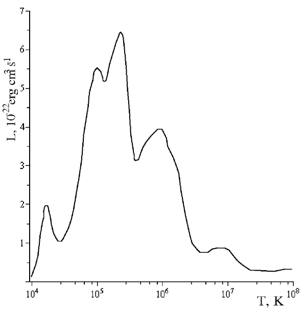
Figure 1: Dependence of the total radiative power loss on the tempetature $L=L(T)$.

Braginskij ,spitzer , $L=L(T)$ is the distribution of radiative energy losses with temperature (see Fig.1), à $P=L(T_{\infty})n^{2}$ – stationary thermal heating at the infinity.

Parameter $L$ of the equation (2) are known: $L=L(T)$ was taken from po4ta .To determine the number density dependence on the temperature $n=n(T)$ let us consider the cases of slow and fast heating.

One has to specify doundary conditions for the temperature in the equation (2):

$$\frac{dT}{d\xi}\Big{|}_{\xi\rightarrow\infty}=0,\quad T\Big{|}_{\xi=0}=T_{0}.$$ (4)

According to Shm , to obtain the dependence $T=T(\xi)$ from the equation of the thermal balance (2) one has to multiply both parts of the equation (2) by $\kappa\frac{dT}{d\xi}$. Then after simple manipulations we have the following expression for the thermal flux $F$:

$$F=\left(\int_{T_{\infty}}^{T}2(L(T^{\prime})-L(T_{\infty}))\kappa n^{2}dT^{\prime}\right)^{\!1/2},$$ (5)

where the thermal flux $F$ is defined as:

$$F=-\kappa n\frac{dT}{d\xi}.$$ (6)

To express (5) in dimensionless form we multiply (5) by

$$\frac{\xi_{\infty}^{2}}{n_{\infty}^{2}\kappa_{\infty}T_{\infty}L(T_{\infty})},$$

where $\xi_{\infty},n_{\infty},T_{\infty},\kappa_{\infty}$ are the units of the depth, concentration, temperature and electron conductivity, correspondingly.

We obtain

$$F=\left(\int_{1}^{T}2K_{1}(L(T)-1)(\frac{T^{5/2}}{ln\Lambda})n^{2}dT\right)^{\!1/2},$$ (7)

where $\ln\Lambda$ is the Coulomb logarithm,

$$\ln\Lambda=\left\{\begin{array}[]{c}\ln\left(1.24\times 10^{4}\ (T\ T_{\infty})^{3/2}/(n\ n_{\infty})^{1/2}\right),\ \ \ T_{e}<5.8\times 10^{5}\ K,\\ \ln\left(9.44\times 10^{6}\ (T\ T_{\infty})/(n\ n_{\infty})^{1/2}\right),\ \ \ T_{e}\geq 5.8\times 10^{5}\ K\end{array}\right.$$

And $K_{1}$

$$K_{1}=\frac{\xi_{\infty}^{2}L(T_{\infty})}{\kappa_{\infty}T_{\infty}}.$$ (8)

Let us choose the units to be the following (recall that these values are simply our choosen units and not the actual values at the infinity):

$$T_{\infty}=10^{4}K,$$

$$n_{\infty}=10^{10}cm^{-3},$$

$$\xi_{\infty}=n_{\infty}l_{\infty}=3.15\times 10^{15}\,{\rm cm}^{-2},\quad l_{\infty}=\left(\frac{\kappa_{\infty}T_{\infty}}{L(T_{\infty})n_{\infty}^{2}}\right)^{1/2}=3.15\times 10^{5}\,{\rm cm}.$$ (9)

From equation (6) we obtain the following expression for $\xi$:

$$\xi=\int_{T}^{T_{c}}\kappa n\frac{dT}{F(T)},$$ (10)

We choose the origin of $\xi$-coordinate to be the point where the temperature has a fixed value $T_{c}$, $T_{c}=10^{6}K$ ( $\xi=0$ when $T=10^{6}K$).

Finally, to get the distribution $T(\xi)$ we can find $F(T)$ from equation (5) and then, after putting $F(T)$ into (6), obtain $\xi(T)$ and thus $T(\xi)$.

In the case of fast heating, when concentration is constant throughout the layer depth ($n=const$), let us set $n=n_{\infty}$, or in dimensionless form $n=1$.

In the case of slow heating gas pressure is constant throughout the layer depth ($p=const$). In this case, because

$$p=nk_{B}T,$$ (11)

concentration becomes

$$n=\frac{p}{k_{B}T}$$ (12)

or in dimensionless form:

$$n=\frac{1}{T}.$$ (13)

The dependence of the thermal flux on the temperature $F=F(T)$ for the cases $n=const$ and $p=const$ is shown in Fig.2. Here

$$F_{\infty}=\frac{\kappa(T_{\infty},n_{\infty})\ n_{\infty}}{\xi_{\infty}}=425\,{\rm erg/s}.$$

The dependence of the temperature along the depth $T=T(\xi)$ for the cases $n=const$ and $p=const$ is shown in Fig.3.

III The width of the transition region ($\delta\xi(T)$ and $\xi_{e}$ comparison)

Classical collisional heat conduction Braginskij ,spitzer is valid if two following conditions are satisfied:

$$\lambda_{e}<l_{T}=\frac{T_{e}}{|\nabla T_{e}|}$$ (14)

where $\lambda_{e}$ is the mean free path for thermal electron collisions, $l_{T}$ is the characteristic scale of length on the temperature profile.

Condition (14) may be written as:

$$\delta\xi>\xi_{e},$$ (15)

where $\delta\xi$ is the characteristic depth for equilibrium temperature distribution obtained above, and $\xi_{e}$ is the thickness corresponding to the free path for thermal electron collisions.

$$\delta\xi(T)=\frac{d\xi(T)}{d\ln(T)},$$ (16)

$$\xi_{e}=n_{e}\lambda_{e}=\frac{k_{{}_{\rm B}}^{2}T^{2}}{\pi e^{4}\ln\Lambda}.$$ (17)

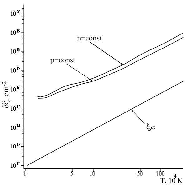
Figure 4: Characteristic values of the thickness versus the temperature for the equilibrium temperature distriution $\delta\xi=\delta\xi(T)$ for the cases fast ($n=const$) and slow ($p=const$) heating. And the thickness corresponding to the mean free path of thermal electrons $\xi_{e}=\xi_{e}(T)$.

The dependence $\delta\xi=\delta\xi(T)$ for the cases $n=const$ and $p=const$ and the dependence $\xi_{e}=\xi_{e}(T)$ are shown in Fig.4.

As we can see from Fig.4 $\delta\xi\gg\xi_{e}$, that is the characteristic thickness at which temperature is changing is more then thickness corresponding to the free path for thermal electron collisions in 400-500 times. For example, on the temperature $T=10^{5}K$ temperature is changing on the 35 km and the free path for thermal electron collisions 70 m.

Thus the chromosphere-corona transition region of the solar atmosphere shall be considered in the collisional approximation.

IV Stability of the solution

Linear theory of the thermal instability was constructed in monography fild due to Field. The uniform medium in the thermal and mechanical balance in linear theory is characterised by 3 dimensionless parameters $\alpha$, $\beta$, $\gamma$.

If the heating is such that energy gain per second to the gramm of substance is now dependent on temperature and density, and cooling of the medium becomes formed by volume radiation energy losses ($n^{2}\ L(T)$), than the parameter $\alpha$ will depend only on temperature. And in this case $\alpha$ is the logarithmic derivative of $L(T)$

$$\alpha(T)=\frac{d\ lnL}{d\ lnT}.$$ (18)

Parameter $\beta$ characterises comparative significance of the thermal conductivity. If the conductivity is defined only by free electrons (3), then

$$\beta(T)=\frac{(\gamma-1)^{2}}{\gamma}\frac{\mu\kappa_{0}}{k_{B}^{3}}\sqrt{T}\ L(T)$$ (19)

That is, $\beta$ also depends only on the temperature; here $\mu$ is the effective molecular weight (for plasma with cosmic abundance of elements $\mu\approx 1,44m_{H}$).

Dependence of $\alpha$ and $\beta$ on the temperature is shown in the Fig.5. We assume $\gamma=5/3$ in the equation (19).

On figure 7 we can see regions where perturbations of the following types can be unstable: 1) Isobaric perturbations, for which $p=const$. Regions where $\alpha\ <\ 1$ correspond to isobaric perturbations. This mode is called condensation mode of thermal instability. 2) In regions where $\alpha<-3/2$ adiabatic (entropy $=const$) perturbations are unstable. This mode of thermal instability is named wave or sonic. 3) In regions with $\ \alpha<0$ isochoric ($n=const$) perturbations are unstable 152 .

Let fild ,16:

$$\xi_{\rho}=\frac{n}{k_{\rho}}=\frac{\gamma^{1/2}}{\gamma-1}\frac{k_{B}^{3/2}}{\mu^{1/2}}\frac{T^{3/2}}{L(T)},$$ (20)

$$\xi_{T}=\frac{n}{k_{T}}=\alpha^{-1}\ \xi_{\rho},$$ (21)

$$\xi_{\kappa}=\frac{n}{k_{\kappa}}=\beta\ \xi_{\rho}.$$ (22)

On the scales which are smaller than critical fild ,26, thermal instability is stabilized by condactivity:

$$\xi_{cc}=\xi_{\rho}\ \beta^{1/2}\ (1-\alpha)^{-1/2},$$ (23)

$$\xi_{cw}=\xi_{\rho}\ \beta^{-1/2}\ (-\alpha-\frac{1}{\gamma-1})^{-1/2}$$ (24)

for the condensation and wave mode. These values of thickness which also depend only on temperature, are shown in the Fig.6.

The values of characteristic thickness which correspond to the biggest increase rate of thermal instability are fild ,46:

$$\xi_{mc}=\left(\frac{(1-\alpha)^{2}}{\gamma^{2}}+\frac{\alpha(1-\alpha)}{\gamma}\right)^{-1/4}\left(\xi_{\rho}\xi_{cc}\right)^{1/2},$$ (25)

$$\xi_{mw}=|\frac{\alpha-1}{\gamma}|^{-1/2}(\xi_{\rho}\ \xi_{cw})^{1/2}$$ (26)

for the condensation and wave mode, correspondingly; they are also shown in the Fig.6.

The characteristic thicknesses corresponding to the stationary chromosphere heating in the cases $p=const$ and $n=const$ for the temperature profiles are shown in Fig.6. At all points of distribution the balance between the thermal heating and radiative cooling has its place.

Let us look at Fig.6. If $\lambda<\lambda_{cr}$, then perturbations are smoothened out by electron conductivity, if $\lambda\approx\lambda_{cr}$, then pertrubations will grow. Note, that our solutions (in the cases $ð=const$ and $n=const$) are crossed by the curve $\xi_{cc}$ corresponding to condensation instability. Then, if in the places of instability there is a spontaneous change of the temperature profile, the profile will return to its original position.

So, we have undrestood that the temperature profile cannot be flatter than equilibrium plofile. It also cannot be steeper, because then the same temperature will be accumulated at smaller thickness, so the emission in this temperature range will be lower.

V The temperature profile emission

The ability to emit of a certain region is named the emission measure ($ME$).

$$ME=\int\limits_{0}^{x}\ n_{e}^{2}\ dl,$$ (27)

here $x$ is the length of emitting region along the line of sight, $dl$ is the interval of length.

Differential emission measure ($DME$) is the derivative of emission measure with respect to temperature.

$$DME=\frac{d\ ME}{d\ T}.$$ (28)

Let us rewrite $DME$ in terms of $\xi$:

$$DME=\frac{d\ ME}{d\ T}=\frac{n_{e}^{2}\ dx}{dT}=n_{e}\ \frac{n_{e}\ d\ x}{d\ T}=n_{e}\ \frac{d\ \xi}{d\ T}$$ (29)

Now, we can calculate the distribution $DME=DME(T)$ for the cases $n=const$ and $p=const$, using the dependences $\xi(T)$ and $n_{e}=n(T)$. The result and measured DME points (for different lines) is shown in the Fig.7.

VI Conclusion

The distribution of temperature with depth was found, assuming that the electon conductivity had place, and at all points of distribution the balance between the thermal heating and radiative cooling had place. Our solution is stable (see IV) and observed UV-radiation can be explained by it (see V).

The obtained results can be used to show that temperatures are distributed in such a way that classical collisional heat conduction is valid in the chromosphere-corona transition region of the solar atmosphere, because the characteristic thickness, at which temperature is changing greater then thickness, corresponds to the free path for thermal electron collisions.

VII Acknowledgements

O.P. thanks P. Dunin-Barkowski for useful discussions. This work is partly supported by RFBR grants 10-02-01315, 08-02-01033-a and by the Russian President’s Grant of Support for the Scientific Schools NSh-65290.2010.2.

Figure 2: Dependence of the thermal flux on the temperature $F=F(T)$.

Figure 3: Distribution of the temperature along the depth $T=T(\xi)$. For the cases fast ($n=const$) and slow ($p=const$) heating.

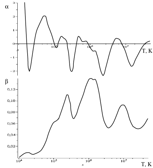
Figure 5: Distributions $\alpha=\alpha(T)$ and $\beta=\beta(T)$.

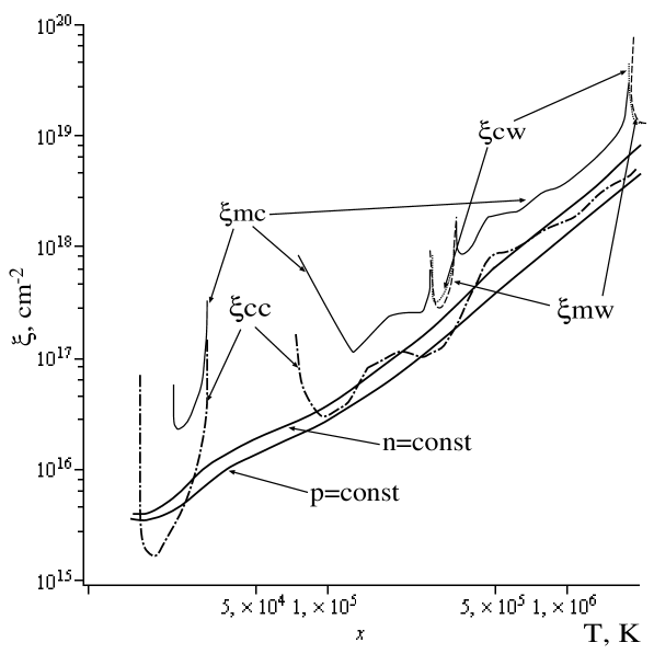
Figure 6: The scales of condensation $\xi_{cc}$ and wave $\xi_{cw}$ perturbations, which is stabilizate by conductivity ((23),(24)), and scales of perturbations with the highest rate of growth $\xi_{mc}$,$\xi_{mw}$ ((25),(26))

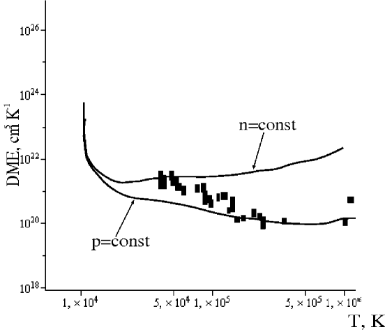
Figure 7: Dependence of the differential emission measure on the temperature $DME=DME(T)$ and measured DME points (for different lines).

References

- (1) P.A. Bespalov, O.N. Savina, Astron. Lett. 34, N5 378 (2008).
- (2) P.A. Bespalov, O.N. Savina, Astron. Lett. 35, N5 343 (2009).
- (3) S.I. Braginskij, in: Leontovich M.A.(eq.) Voprosi teorii plazmy 1, M., (1963).
- (4) L. Spitzer Physics of Fully Ionized Gases, Wiley (1956).
- (5) B.V. Somov, N.S. Dzhalilov, U. Shtaude, Astron. Lett. 33 N 5, 352, (2007).
- (6) O.P. Shmeleva, S.I. Syrovatskii, Solar Phys. 33, 341 (1973).
- (7) B. Field , Astrophys. J. 142, 531 (1965).
- (8) E.N. Parker, Astrophys.J. 117, 431 (1953).
- (9) E. Landi, F. Chiuderi Drago Astrophys.J. 675, 1629 (2008).
- (10) B.V. Somov, Solar Phys. 60, 315 (1978).
- (11) B.V. Somov, Physical Processes in Solar Flares, Kluwer Acad. Publ. Dordrecht, Boston (1992).
- (12) B. V. Somov, S. I. Syrovatskii, Uspekhi Fizicheskikh Nauk 120, 217 (10/1976).