Statistical Properties of Blue Horizontal Branch Stars in the Spheroid: Detection of a Moving Group $\sim 50$ kpc from the Sun

Abstract

A new moving group comprising at least four Blue Horizontal Branch (BHB) stars is identified at $(l,b)=(65^{\circ},48^{\circ}$). The horizontal branch at $g_{0}=18.9$ magnitude implies a distance of 50 kpc from the Sun. The heliocentric radial velocity is $\langle V_{r}\rangle=-157\pm 4$ km s^-1, corresponding to $V_{\mbox{\it gsr}}=-10$ km s^-1; the dispersion in line-of-sight velocity is consistent with the instrumental errors for these stars. The mean metallicity of the moving group is [Fe/H]$\sim-2.4$, which is significantly more metal poor than the stellar spheroid. We estimate that the BHB stars in the outer halo have a mean metallicity of [Fe/H]=$-2.0$, with a wide scatter and a distribution that does not change much as a function of distance from the Sun. We explore the systematics of SDSS DR7 surface gravity metallicity determinations for faint BHB stars, and present a technique for estimating the significance of clumps discovered in multidimensional data. This moving group cannot be distinguished in density, and highlights the need to collect many more spectra of Galactic stars to unravel the merger history of the Galaxy.

1 Introduction

In recent years, stellar photometry primarily from the Sloan Digital Sky Survey (SDSS) has allowed astronomers to discover previously unknown spatial substructure in the Galactic spheroid. Other surveys such as 2MASS and QUEST have also been influential. Highlights include the discovery of new tidal streams (Newberg et al., 2002; Odenkirchen et al., 2003; Grillmair & Johnson, 2006; Grillmair & Dionatos, 2006; Grillmair, 2006; Belokurov et al., 2006; Newberg et al., 2009); dwarf galaxies, star clusters, and transitional objects (Willman et al., 2005a, b; Zucker et al., 2006a, b; Belokurov et al., 2006, 2007; Irwin et al., 2007; Koposov et al., 2009; Belokurov et al., 2009); and previously unidentified spatial structure of unknown or controversial identity (Vivas et al., 2001; Yanny et al., 2003; Majewski et al., 2004; Newberg & Yanny, 2005; Belokurov et al., 2007; Jurić et al., 2008; An et al., 2009).

The discovery of spatial substructure immediately suggests the need for spectroscopic follow-up to determine the orbital characteristics of tidal debris, the masses of bound structures, and the character of structures of unknown identity. It has long been known that a spheroid that is formed through accretion will retain the record of its merger history much longer in the velocities of its component stars than it will in their spatial distribution (Helmi et al., 2003). For this reason early searches concentrated on velocity to find “moving groups” in the spheroid (Majewski et al., 1996) rather than on the search for spatial substructure.

Groups of spheroid stars that have similar spatial positions and velocities (moving groups) are generally equated with tidal disruption of star clusters or dwarf galaxies, unlike local disc “moving groups” that were once hypothesized to be the result of disruption of star clusters (Boc, 1934; Eggen, 1958) but are now thought to be the result of orbital resonances (Famaey et al., 2008).

Recently, searches for spheroid velocity substructure in SDSS data have concentrated on local (up to 17.5 kpc from the Sun) metal-poor main sequence stars (Klement et al., 2009; Smith et al., 2009; Schlaufman et al., 2009), finding more than a dozen groups of stars with coherent velocities. Schlaufman et al. (2009) estimate that there are $10^{3}$ cold substructures in the Milky Way’s stellar halo. Blue horizontal branch (BHB) stars are particularly important for studies of spheroid substruscture (e.g. Clewey & Kinman 2006) because they can be seen to large distances in the SDSS and because a large fraction of the SDSS stellar spectra are BHBs. In the future we need more complete spectroscopic and proper motion surveys designed to discover velocity substructure in the Milky Way’s spheroid.

In this paper we present evidence for a tidal moving group of BHB stars, discovered in the SDSS and Sloan Extension for Galactic Understanding and Exploration (SEGUE; Yanny et al. 2009) spectroscopic survey. Additional evidence that the stars are part of a coherent structure comes from the unusually low metallicity of the stars in the moving group. We are unable to isolate this moving group in density substructure, highlighting the power of velocity information to identify low density contrast substructure in the spheroid.

Historically many of the spheroid substructures have been discovered by eye in incomplete datasets, rather than by a mechanical analysis of data with a well-understood background population. As the size of the substructures decreases, it becomes more critical to determine whether the observed structure could be a random fluctuation of the background. In this paper, we present a method (Appendix A) for estimating the probability that a random fluctuation could produce an observed “lump.”

As we work towards the fainter limits of the SDSS data, it becomes more important to understand how stellar parameters derived from spectra are affected by a low signal-to-noise (S/N) ratio. The stars in the newly detected halo substructure have S/N ratio between 7 and 10, as measured from the ratio of fluctuations to continuum on the blue side of the spectrum. In the past we have successfully used spectra with S/N as low as 5 to measure radial velocities of F turnoff stars in the Virgo Overdensity (Newberg et al., 2007). In this paper, we show that although higher S/N is preferable, some information about metallicity and surface gravity can be gained for BHB stars with S/N ratios less than 10.

Since the strongest evidence that these BHBs form a coherent group is that they have unusually low metallicity, even for the spheroid, we also explore the SEGUE metallicity determinations for BHB stars in the outer spheroid. A great variety of previous authors have measured a large metallicity dispersion for spheroid stars, with average metallicities somewhere in the $-1.5<\rm[Fe/H]<-1.7$ range (Freeman, 1987; Gilmore, Wyse, & Kuijken, 1989). These investigations analysed globular clusters (Searle & Zinn, 1978; Zinn, 1985), RR Lyraes (Saha, 1985; Suntzeff et al., 1991), K giants (Morrison et al., 2003), and dwarfs (Carney et al., 1990). Norris (1986) found an average [Fe/H] of $-1.67$ for globular clusters in the outer halo, and an average metallicity of $-1.89$ for field stars in the outer halo, again with a large metallicity dispersion that does not depend on distance. The Besançon model of the Milky Way adopted an average [Fe/H] of $-1.7$, with $\sigma=0.25$, for the stellar halo (Robin et al., 2000). Recently, Carollo et al. (2007, 2010) analysed the full space motions of $>10,000$ stars within 4 kpc from the Sun, and found evidence that the ones that are kinematic members of the outer halo have an average metallicity of [Fe/H]=$-2.2$.

Our analysis of the SDSS BHB stars shows that the metallicity of BHB stars in the Galactic spheroid does not change from $g_{0}=14.5$ (6 kpc from the Sun) to $g_{0}=19.15$ (55 kpc from the Sun) at high Galactic latitudes. The mean measured metallicity of these stars is [Fe/H]=$-1.9$, but analyses of globular clusters in the sample show that there could be a systematic shift in the BHB measured metallicities of a few tenths of a magnitude, and in fact [Fe/H]=$-2.0$ is our best guess for the proper calibrated value.

2 Observations and Data

Figure 1: Identification of a moving group. The upper left and right plots show blue horizontal branch (BHB) stars with spectroscopic data in the region $50^{\circ}<l<80^{\circ}$ and $40^{\circ}<b<55^{\circ}$, where the velocity is the line of sight velocity with respect to the Galactic standard of rest. The data in the two plots are the same, with the upper left plot marking two overdensities noticed on the upper right plot. Open circles in the lower left plot show the sky positions of the same BHB candidates with spectroscopic data in SDSS DR6. Filled circles correspond to stars that are in the co-moving stellar association, with the same stars plotted in the upper left and lower left plots. These stars have $g_{0}$ magnitudes of $18.65<g_{0}<19.15$ and line of sight velocities, with respect to the Galactic standard of rest, of $-35<V_{\mbox{\it gsr}}<15$ km s^-1. The crossed circles show the positions of stars in a density at $g_{0}=16.5$ found on the upper left plot. In the lower left figure, a higher fraction of the BHB stars have spectra near the globular cluster M13, at $(l,b)=(59^{\circ},41^{\circ})$. The box indicates the area of the newly discovered over-density. The smaller black dots in the lower left plot indicate the positions of photometrically selected BHB stars in Galactic coordinates. The lower right plot shows the positions of the photometric data from the lower left plot that has the $g_{0}$ magnitude range of the moving group, $18.65<g_{0}<19.15$. Note that the moving group is not detected from the photometric data alone.

In order to search the stellar halo for co-moving groups of stars, we selected BHB stars from the sixth data release (DR6; Adelman-McCarthy et al. 2008) of the SDSS. This release contains both Legacy Survey and SEGUE photometric data from 9583 square degrees of sky. More technical information for the SDSS survey can be found in York et al. (2000); Fukugita et al. (1996); Gunn et al. (1998); Smith et al. (2002); Stoughton et al. (2002); Abazajian et al. (2003); Pier et al. (2003); Ivezić et al. (2004); Gunn et al. (2006); Tucker et al. (2006).

We selected 8753 spectra with the colors of A stars from the SDSS DR6 Star database using the color cuts $-0.3<(g-r)_{0}<0.0$ and $0.8<(u-g)_{0}<1.5$, within the magnitude range $15<g_{0}<23$, where the $0$ subscript indicates that the magnitudes have been corrected for reddening and extinction using the Schlegel et al. (1998) reddening map. Within this color box, the stars that are bluer in $(u-g)_{0}$ tend to be high surface gravity blue straggler (BS) or main sequence stars, and those that are redder in $(u-g)_{0}$ tend to be low surface gravity blue horizontal branch (BHB) stars. Using $(u-g)_{0}$, $(g-r)_{0}$ color selection parameters as described in Figure 10 of Yanny, Newberg et al. (2000), we divided the sample into $4630$ candidate BHB stars and $4123$ candidate BS stars with spectra.

We separated the stars in surface gravity using a photometric technique, because in 2007 when we were selecting the stars, we were concerned that the S/N of the spectra would degrade more quickly than the S/N of the photometry at the faint end of our sample. The S/N of the spectroscopy increases over the whole magnitude range from $15<g_{0}<20.5$, while the photometric accuracy degrades only for $u>19$. The photometric degradation affects halo BHB stars fainter than about $g_{0}=18$. With more recent reduction software (see below), we have found similar sensitivity to surface gravity in photometric and spectroscopic indicators for faint SDSS spectra, but the spectroscopic separation is much better than photometric separation for bright, high S/N spectra. The photometric selection technique does not introduce gradients in the selection effect with apparent magnitude, and can be applied identically for stars with and without measured spectra.

At bright magnitudes, the spectral S/N is high enough that the DR6 surface gravities are reliable. The SDSS spectra are R=1800, and the S/N of A star spectra varies from 50 at $g_{0}=16$ to 7 at $g_{0}=19$. We tested the efficiency and completeness of the photometric selection technique using 3996 SDSS spectra of stars with $16<g_{0}<17.5$ and colors of A-type stars. Of the 1948 that had surface gravities consistent with BHB stars, 84% were classified as BHBs by the photometric technique. Of the 2048 spectra with high surface gravity (BS stars), 35% were classified as BHBs in the photometric technique. These numbers for completeness and contamination are similar to estimates that we made from examination of Figure 13 from Yanny, Newberg et al. (2000), and apply only to stars with $u<19.$ Fainter than this, the photometric errors in $u$ will cause increased mixing of the populations.

3 Detection of a new moving group in the Galactic halo

We searched our BHB catalog for stars that clustered in velocity, apparent magnitude, and Galactic coordinates. Our search was less systematic than that used by Clewley & Kinman (2006), but allows us to find moving groups that are more extended, such as tidal streams. Because they first searched for pairs of co-moving stars that were within $2$ kpc of each other, they reduced their sensitivity to tidal debris streams that could be spread over tens of kpc.

We first divided the catalog into sky areas in $(l,sin(b))$ that were $20^{\circ}$ by $0.2$ in the respective coordinates, and made plots of $V_{\mbox{\it gsr}}$ vs. $g_{0}$ magnitude. We used $sin(b)$ so that each partition of the data would cover an equal area of the sky. Here, $V_{\mbox{\it gsr}}$ refers to the line-of-sight velocity transformed to the Galactic standard of rest using the Solar motion of $(v_{X},v_{Y},v_{Z})=(10,225,7)$ km s^-1 (Dehnen & Binney, 1998). By examining the line-of-sight velocity as a function of magnitude, we found a number of co-moving groups of stars that were associated with known globular clusters, dwarf galaxies, and tidal streams. Halo substructures that had been previously identified were not studied further. We concentrated only on the most significant of the remaining BHB association; others were left for future studies.

Figure 1 shows the $V_{\mbox{\it gsr}}$ vs. $g_{0}$ plot for the most significant co-moving group of BHB stars, along with the distribution of these stars in $(l,b)$. Although there is a second cluster of stars at $g_{0}\sim 16.5$ in the top left plot, we show in the lower left plot that these stars are dispersed in position on the sky so we did not explore that association further.

The moving group we describe here has BHB stars at $g_{0}=18.9$, $\sigma_{g_{0}}=0.1$; and $V_{\mbox{\it gsr}}=-10$ km s^-1, $\sigma_{\mbox{\it gsr}}=10$ km s^-1. The dispersion is consistent with the instrumental error in the velocity of 19^th magnitude BHB stars (Sirko et al., 2004). These stars have an average heliocentric radial velocity of $<\langle V_{r}\rangle>=-157\pm 4$ km s^-1, which rules out any association of these stars with the disc population. In the direction $(l,b)=(65^{\circ},48^{\circ})$, the line-of-sight, heliocentric velocities expected for the thin disc, thick disc, and spheroid components are $-2$, $-35$, and $-144$ km s^-1, respectively. The heliocentric radial velocity of our moving group is not far from that of the average spheroid star in that direction ($V_{\mbox{\it gsr}}=0$ for the spheroid and $V_{\mbox{\it gsr}}=-10$ km s^-1 for the moving group), but the dispersion rules out an association with the general spheroid population. The lower right panel of Figure 1 shows that the association of horizontal branch stars could not be detected spatially; velocity information was required to identify the moving group.

In the same area, at $(l,b)\sim(59^{\circ},46^{\circ})$, another cluster identified from SDSS BHB stars was found by Clewley & Kinman (2006). Although this cluster lies at roughly the same (l,b) angular position as the cluster identified in this paper, the estimated distance to the Clewley et al. clump is 7.8 kpc, which is much closer to the Sun than our moving group, with a horizontal branch brighter than $g_{0}=16$.

The parameters of the seven BHB stars in the moving group are presented in Table 1. The new moving group found in this study is located at $(l,b)\sim(65^{\circ},47.5^{\circ})$. The stars have apparent magnitude in the $g$ filter of $g_{0}\sim 18.9$ and velocities located within $-35<V_{\mbox{\it gsr}}<15$ km s^-1, with an average velocity of $<V_{\mbox{\it gsr}}>=-10$ km s^-1. A $g_{0}$ apparent magnitude of $18.9$ for BHB stars, with an estimated absolute magnitude of $M_{g_{0}}=0.45$ (Newberg et al., 2009) corresponds to a distance of $\sim 50$ kpc from the Sun. The magnitude dispersion of the seven stars is $\sigma=0.10$. Note that the dispersion in apparent magnitude for these stars is $\sigma_{g_{0}}=0.1$, and drops to $\sigma_{g_{0}}=0.03$ if the two outliers with larger magnitudes (one of which has a high estimated surface gravity) are excluded. The magnitudes are consistent with a structure that has zero depth, but the depth could be as large as $\sigma=2$ kpc.

Table 1: Properties of BHBs in the Hercules Moving Group.

ID	RA	DEC	l	b	$g_{0}$	$(u-g)_{0}$	$(g-r)_{0}$	$V_{\mbox{\it gsr}}$	$\log(g)$	$[Fe/H]$	S/N
plate-mjd-fiber	hh:mm:ss.s	dd:mm:ss.s	∘	∘	mag	mag	mag	km s-1	dex	dex
1336-52759-290	16:08:33.7	+38:49:19.7	61.8	47.6	19.00	1.22	-0.21	2.0	2.75	-2.99	7.7
1335-52824-1001	16:06:59.7	+40:20:39.5	64.1	47.8	18.89	1.17	-0.16	-4.4	2.34	-1.97	8.5
1335-52824-1671	16:04:32.4	+40:46:03.1	64.8	48.3	18.85	1.27	-0.17	-10.0	2.91	-2.86	9.8
1335-52824-3621	16:00:37.6	+41:55:10.5	66.6	48.9	18.82	1.17	-0.20	-8.3	2.83	-2.63	9.2
1334-52764-540	15:58:24.7	+43:04:07.4	68.4	49.2	19.10	1.16	-0.14	-9.7	3.39	-2.10	7.7
1335-52824-0081	16:09:25.9	+40:05:30.9	63.7	47.4	18.86	1.24	-0.20	-19.1	2.92	-2.27	8.1
0814-52443-046	16:17:17.7	+44:19:04.7	69.7	45.7	18.89	1.16	-0.14	-18.7	2.62	-2.42	9.1
1056-52764-637	16:18:21.5	+36:54:11.0	59.1	45.7	18.90	1.32	-0.12	-5.3	2.21	-2.99	9.9

¹ Highly likely member of moving group.

4 Surface Gravity Estimates of Faint BHB Stars in SDSS

The SDSS DR7 SSPP pipeline (Lee et al., 2008a, b) generates ten different measures of the surface gravity for each stellar spectrum, and additionally computes an “adopted” $\log g$, which is determined from an analysis of the ten different methods. For stars with S/N less than 10, the adopted $\log g$ is set to an error code.

We analyzed histograms of the distribution in $\log g$ of bright and faint A stars in our sample, looking for a method that showed two peaks: one at low surface gravity (BHB stars), and one at high surface gravity (BS or main sequence stars). Several of the methods appeared to separate bright A stars by surface gravity, and none appeared to separate the stars with S/N$<10$ very well. We selected the logg9 parameter, which is described in general terms in Lee et al. (2008a), in which it is referred to as the “k24 grid”. The original reference to the method is Allende Prieto et al. (2006), where the method is described in great detail. The method finds the best match between the SDSS spectrum and a set of model atmospheres from Kurucz (1993), using the $(g-r)$ color index and the normalized spectral fluxes in the wavelength range $4400<\lambda<5500$ Å , using a resolving power of $R=1000$. The surface gravities using this DR7 logg9 estimator are tabulated in Table 1. Six of the seven candidate members of the moving group have surface gravities less than $3.0$, as expected for BHB stars.

Subsequent to our search for spheroid structure using BHB stars, Xue et al. (2008) published a list of SDSS DR6 A stars along with measurements of $D_{0.2}$ and $f_{m}$ measurements. These are classical indices used by Pier (1983) to classify BHB stars from the $H_{\delta}$ line width and depth. Using this method for determining the surface gravities of A stars, only 2 of our candidate A stars appear to be low surface gravity. There are two effects that contribute to the small fraction of confirmed BHBs: (1) the performance of the $D_{0.2}$ indicator is degraded at low signal-to-noise, and (2) we disagree with the published $D_{0.2}$ values for two of the stars.

In the top panels of Figure 2, we show the performance of the $D_{0.2}$, $f_{m}$ indicators for the set of $10,224$ stars from Xue et al. (2008), and for the subset of 1176 of these stars for which the S/N of the spectrum is between 7 and 10. While the bright, high signal-to-noise spectra that were used by Xue et al. (2008) are separable, the lower signal-to-noise spectra do not have two clear peaks in the diagram. We show histograms of $D_{0.2}$ for all of the stars between the two vertical lines ($0.16<f_{m}<0.24$) in the top two panels of Figure 3. For all of the stars (most of which are high signal-to-noise), we see two peaks in the $D_{0.2}$ distribution. The low S/N sample shows no separation.

We compare the separation using the properties of one line of the spectrum ($H\delta D_{0.2}$ vs. $f_{m}$) with the SSPP logg9 surface gravities using photometry and the continuum levels of the spectra in the bottom panels of Figures 2 and 3. Figure 2 shows that the logg9 indicator works about as well as the $D_{0.2}$ indicator for bright stars. Note that in the lower right panel, for stars with marginal S/N, the distribution of stars is much wider in the vertical direction, and the width in the horizontal axis is wider but not dramatically so. The lower panels of Figure 3 show histograms of logg9 for all of the stars between the two horizontal lines ($15<D_{0.2}<40$). The brighter star data on the left shows two separate peaks for low and high surface gravity stars, while the marginal S/N data in the right panel does not show that separation. However, we can see from the correlation between $D_{0.2}$ and logg9 in the lower right panel of Figure 2 that there is some information on the surface gravity of even these lower S/N spectra.

Because we were surprised that the $D_{0.2}$ numbers could be so high, even at low signal-to-noise, for stars that we expected were BHBs in a moving group, we independently computed new values for the width of the $H_{\delta}$ at 80% of the continuum for the eight stars in Table 1. For six of them, we measured widths that were reasonably consistent with the published values. However, we measured a width of 23 for 1335-52824-167 instead of 40, and a width of 23 for 1335-52824-008 instead of 33. With these corrections, six of the eight stars in Table 1 have $D_{0.2}$ widths less than 30, including all four of the stars that we will later show are highly likely members of the moving group.

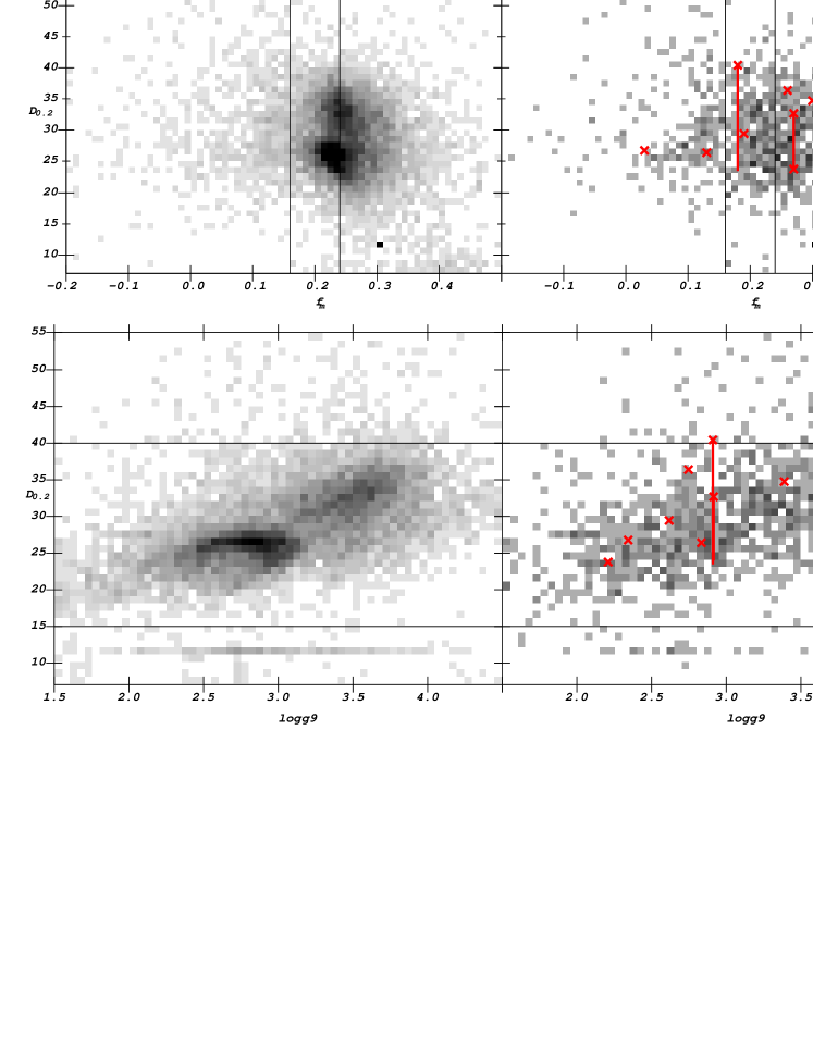
Figure 2: Luminosity separation of A colored stars into BHB and BS populations. Upper left panel reproduces the sample of 10,224 A colored stars from Xue et al. (2008), showing that BHBs have lower $H\delta$ $D_{0.2}$ widths than BSs. The upper right panel shows a low S/N subset of 1,176 stars ($7<\rm S/N<10$). The candidate stream members from Table 1, which all have S/N in this range, are indicated with (red) crosses. The single $D_{0.2}$ method appears to be a less effective discriminant at S/N $<10$. However, our independent measurement of $D_{0.2}$ for the moving group candidates resulted in significantly lower $H_{\delta}$ widths for two of the eight stars (indicated be the vertical line below two of the crosses), so the effectiveness of the $D_{0.2}$ may depend on how it’s measurement is implemented for low signal-to-noise. The lower left panel shows $D_{0.2}$ versus the 9^th SSPP method (logg9)for the same Xue et al. (2008) sample. Note that the logg9 surface gravity discriminant achieves similar results to the $D_{0.2}$ measure for bright stars. On the lower right, the lower S/N sample is shown. A cut at $\rm logg9<3.15$ maintains the $D_{0.2}$ separation into BHBs and BSs which appears effective even at S/N $<10$. In this paper, we use an even more conservative cut at logg9$<3.0$. Using this conservative selection criterion for BHB stars, 7/8 stream candidates (red crosses) are consistent with low surface gravity BHB stars.

Figure 3: Histograms showing gravity separation of data between the parallel lines in each panel of Figure 2. Upper left: We show $D_{0.2}$ for the subset of the Xue et al. (2008) sample with an $H\delta$ flux minimum (as fraction of continum) of $0.16<f_{m}<0.24$. Upper right: We show the same histogram for the lower ($7<\rm S/N<10$) signal-to-noise subsample. Stream candidates from Table 1 are indicated with a heavy curve. Note the two values at 40 Å and 33 Å should be moved lower (23 Å ) based on inspection of individual spectra. Lower Left: We show the distribution of logg9 for most of the Xue et al. (2008) sample. Lower Right: We show the lower S/N subsample. Note the positions of the stream candidates (dark line), which are consistent with the low surface gravity BHB population in 7/8 cases. Note the clear bimodality between BHBs (low $D_{0.2}$ or low logg9) and BSs (high $D_{0.2}$ or high logg9) for the full samples, and the absence of bimodality for the lower S/N samples.

5 Statistical Significance of the Moving Group

Given that we were searching through the data by eye and looking for clusters, it is important to verify that the clustering of stars is not a chance coincidence. In this section we will estimate an upper bound for the probability that this clump could be a random fluctuation in the number of stars in a a small region of angle in the sky, magnitude, and line-of-sight velocity.

Most of the sky that we searched for clumps was at high Galactic latitude; at low Galactic latitude the stellar population is different, the density of stars is higher, and the sky coverage is less uniform. So for statistical purposes we limited our sample to $b>35^{\circ}$. There are 2893 stars in our sample with $b>35^{\circ}$. The seven stars were discovered in a 19 square degree area of the sky (compared with 8800 square degrees above $b>35^{\circ}$), with the requirement that this sky area be rectangular in Galactic latitude and longitude ($61.8<l<69.7,45.7<b<49.2$). In comparison with the entire high latitude sample of BHB candidates, the seven stars in the clump span about 1/46^th of the entire longitude range of the input data, and 1/10^th of the latitude range of the data in an equal-area plot. From Figure 1, we find that the range of velocities in the clump includes $15\%$ of the sample stars, and the range of magnitudes in the clump is the same as $10\%$ of those in the high latitude sample.

Appendix A presents a statistical method to determine the significance of a “clump” of data points in a $d$-dimensional search space. In this case we have four dimensions: Galactic longitude, Galactic latitude, radial velocity, and apparent magnitude. The statistical method measures the probability that random data will produce a clump of seven or more points within a four-dimensional box of the measured size. By using percentiles, we account for the non-uniformity of the data in the radial velocity and apparent magnitude dimensions. We also adjust the statistics, as explained in Appendix A.4.2, for the periodic boundary condition in Galactic longitude. What is important for the calculation is that each of the dimensions be independent (separable, in the terms of Appendix A). In our case, the variables are not quite independent, especially Galactic coordinates. Because the density of A stars with SDSS spectra varies as a function of position in the sky, the relative percentiles in $(l,b)$ would be different if a clump of the same areal extent were discovered in a different part of the sky. We estimate that the local density in the region of the sky that the clump was found is 3.5 times higher than average. Therefore, following the prescription of Appendix A4.4, we multiplied the longitude width of the clump by a factor of 3.5.

It was not possible to account for every known peculiarity of the data. For instance, when we searched for clumps we divided the sky up into fixed $(l,b)$ boxes, so there are regions around the edge of each $(l,b)$ box that were not as thoroughly searched. However, it is possible that if nothing was found with these limits we would have adjusted the box sizes and positions, so this oversight (which would underestimate the significance of a clump) is probably justified.

Given the percentiles of the 4-D search space listed above, we expect 0.32 stars in a typical box with these dimensions. Using the algorithm in Appendix A, the number of clumps we should expect to find in this data that have seven or more stars in a 4-D box of these dimensions or smaller is 0.96. Since we found one clump, this is very close to random. If we eliminate one star from the sample that is an outlier in $(l,b)$, so that the area of sky is now $61.8^{\circ}<l<68.4^{\circ}$, $47.4<b<49.2^{\circ}$, then we calculate that the E-value for finding six or more stars in a 4-D box with these (smaller) dimensions is 0.18, so the probability of finding this moving group is not more than one in six. Using only these dimensions, the clump of stars is not a significant detection.

In order to claim a significant detection of the moving group represented by these seven stars, it is necessary to compare their metallicities with the metallicities of the background population. Only 30% of the stars in the sample have metallicities as low as those in the clump of seven stars. If we extend the statistical calculation to five dimensions, including metallicity, then the probability of finding seven stars in a region of this size and shape (or smaller), anywhere in the 5-D parameter space is not more than 1 in 244 (E-value of 0.004), and the probability of finding six stars in a smaller angular region in the sky (in 5-D) is not more than 1 in 490 (E-value=0.002). These are highly significant detections.

Since metallicity is critical to the detection of this substructure, we examine the SDSS DR7 metallicity measurements of these stars, and BHB stars in general, in the next two sections. In section 8, we use the information we have learned in the analysis of this moving group to re-select similar data from SDSS DR7, and make an even stronger argument for the statistical significance of our result.

6 Metallicities of the moving group stars

All seven of the candidate BHB stars in this moving group had unmeasured metallicities in SDSS DR6, but metallicities were assigned to these same spectra in the much improved SSPP pipeline of SDSS DR7 (Lee et al., 2008a, b). Our metallicities come from the DR7, which became public in October 2008. The SDSS DR7 tabulates many measures of the metallicities of stars, of which the most commonly used is FEHA, the “adopted” metallicity, which is derived from a comparison of all methods used to measure metallicity. In this paper we use instead the metallicity of Wilhelm, Beers, & Gray (1999), hereafter WBG, which is specifically designed to measure the metallicities of BHB stars. The WBG metallicities of the seven BHB stars in the moving group are given in Table 1 and are shown in Figure 4. The mean of the distribution is [Fe/H]$=-2.46\pm 0.14$, and the width is $\sigma=0.4$.

Figure 4: Metallicity distribution of the moving group. We selected all stars with spectra from SDSS DR7.1 which had the same photometric properties as the moving group BHB stars ($18.65<g_{0}<19.15$, $-0.3<g-r_{0}<0.0$, $0.8<(u-g)_{0}<1.5$, and split photometrically by likelihood of low surface gravity), with Galactic latitude $b>45^{\circ}$. The 298 stars selected are all likely spheroid BHB stars, of which 260 had measured metallicities. The distribution of metallicities of the spheroid BHB stars with similar photometric properties (thin lines) is shown along with the metallicities of the seven BHB stars in the moving group (thick lines). The moving group has a mean metallicity of $-2.5$, while the spheroid BHBs have a mean metallicity of $-1.69$.

We now show that the metallicities of the moving group stars are not consistent with being drawn at random from the stellar halo. We selected all stars in DR7 with the same photometric constraints as the stars in the moving group, and with $b>45^{\circ}$ so that the BHB stars are likely to come from the same component (the spheroid), and not be confused with disc populations of BHBs. To remove BHB stars in the Sagittarius dwarf tidal stream from the sample, we also eliminated stars with $\delta<5^{\circ}$. There were 298 stars with $18.65<g_{0}<19.15$, $-0.3<(g-r)_{0}<0.0$, $0.8<(u-g)_{0}<1.5$, and that passed the photometric low surface gravity cut. Of these, 260 had measured metallicities that are shown in Figure 4. The mean of the distribution is [Fe/H]$=-1.69\pm 0.04$, and the width is $\sigma=0.71$. Note that the error quoted here is a statistical error. Because very few of the SEGUE calibration stars are as blue as A stars, the systematic errors at this end are about $\pm 0.3$. The comparison stars are about 45 kpc from the Sun, and above $b=45^{\circ}$, so they come from the distant halo. The blue straggler contaminants are 10 to 28 kpc away, which is also fairly far from the disc at high Galactic latitudes.

A comparison of the stars in the moving group with the similarly selected stars in the spheroid with a t-test gives a probability of 1 in $10^{6}$ that the two groups of stars were selected from the same stellar population. The Mann-Whitney test (also known as the Wilcoxon rank sum test) gives a p-value of 0.00023, or a 2 in 10,000 probability that the two samples are drawn from the same population. This leads us to conclude that the moving group is real.

As a further test, we selected the other 8 stars in the lower panel of Figure 1 that have the same $V_{\mbox{\it gsr}}$ and apparent magnitude as the blue horizontal branch stars in the moving group, and find that they have a mean metallicity of $-1.87$ with a sigma of 0.86. The t-test (p=0.948) shows that this distribution is not distinguishable from the background population. (Performing the Mann-Whitney test for this sample is problematic since several of the stars are not part of our selected background distribution.)

7 Systematics of DR7 Metallicities of halo BHB stars

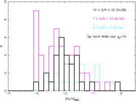
Figure 5: Measured metallicities of BHB star in the Sgr dwarf leading tidal tail, as a function of S/N. The metallicities of stars with S/N$>10$ are considered fairly reliable. The stars with $7<$S/N$<10$ have a similar distribution. Stars with $0<$S/N$<7$ have a significantly higher average metallicity. Therefore, we conclude that the metallicity measurements of BHB stars with S/N$<7$ are not reliable. Note that the excess of stars at [Fe/H]${}_{\rm WBG}=-3.0$ is due to edge effectes in the WBG estimation procedure, and does not represent a cluster of stars with identical metallicity.

In this section we explore the accuracies of the DR7 metallicity measurements of BHB stars as a function of S/N and in comparison with published metallicities for globular clusters. We also explore the metallicity of BHB stars in the halo as a function of apparent magnitude.

Since all of our moving group stars have low S/N, we need to test the accuracy of the metallicity measurements. We do this by selecting BHB stars in the leading tidal tail of the Sgr dwarf galaxy that are about the same distance from the Sun as the moving group. We selected all of the spectra from SDSS DR7 that had elodierverr$>0$ (if the radial velocity error when matching to the stellar templates is less than zero, that indicates that the object is not a star), $0.8<(u-g)_{0}<1.5$, $-0.3<(g-r)_{0}<0.0$, $320^{\circ}<l<350^{\circ}$, $30^{\circ}<b<70^{\circ}$, $-100<V_{gsr}<100$ km s^-1, logg9$<3.0$, and $18.5<g_{0}<19.6$. The 94 stars that are likely BHBs in the Sgr dwarf tidal stream were divided into three files based on S/N. There were 14 stars with $0.0<$S/N$<7$, 49 stars with $7<$S/N$<10$ (excluding three with unmeasured metallicities), and 28 with $10<$S/N$<25$. The metallicity distributions of these three S/N groups is shown in Figure 5.

The highest S/N group ($10<$S/N$<25$) has a mean [Fe/H]${}_{\rm WBG}=-1.94$, which is similar to the group with marginal S/N ($7<$S/N$<10$) which has a mean [Fe/H${}_{\rm WBG}=-2.13$. A Mann-Whittney test comparing these two samples gives a result of $U=818$, $z=-1.39$, and a p-value of 0.165. These distributions are not significantly different from each other. This gives us some confidence that the metallicities of the moving group stars, which have S/N measurements in this marginal range, are usefully measured.

In contrast, the lowest S/N group ($0<$S/N$<7$) has a mean of [Fe/H]${}_{\rm WBG}=-1.42$. A Mann-Whittney test comparing this sample with the highest S/N sample produces $U=275.5$, $z=-2.11$, and a p-value of 0.0349. This is a statistically significant difference, and metallicities of BHB stars measured by this technique are probably not accurate.

To understand the likely systematics in our metallicity determinations, we selected BHB stars from six globular clusters that had spectroscopic measurements of BHB stars in SDSS DR7. We selected stars that have the colors of BHB stars, are within half a degree of the centre of the globular cluster, and have radial velocities within 20 km s^-1 of the published value for the cluster. M2, M3, and M13 have metallicities very close to $-1.6$; M53 has metallicity of $-1.99$; and the two clusters M92 and NGC 5053 have metallicities very close to $-2.3$ (Harris, 1996). Because there were very few stars with spectroscopy in each globular cluster, we combined the data from clusters with similar metallicities before plotting the histograms in Figure 6. All of these globular clusters have horizontal branches near $g_{0}=16$ (the magnitude range for which we have the most complete sample of BHB stars), and thus the spectra have high $S/N$.

Figure 6: Metallicity measures of known clusters. We show the metallicity distribution of SDSS DR7 BHB stars, as measured by the Wilhelm, Beers, & Gray (1999) technique, for BHB stars selected from clusters of known metallicity. Uppermost panel: Stars in M2 ([Fe/H] = $-1.62$), M3 ([Fe/H] = $-1.57$), and M13 ([Fe/H] = $-1.54$). Second panel: Stars in M53 ([Fe/H] = $-1.99$). Third Panel: Stars in M92 ([Fe/H] = $-2.28$) and NGC 5053 ([Fe/H] = $-2.29$). Lowermost Panel: The seven Hercules stream BHBs. Note that the measured metallicities are compressed toward [Fe/H]=$-1.9$ (higher metallicity stars are measured systematically low, and lower metallicity stars are measured systematically high). Also note that the Hercules stream stars appear to be lower metallicity than M92 and NGC 5053.

Figure 6 shows that the SDSS DR7 WBG metallicities for BHB stars tend to push the metallicities toward [Fe/H]=$-1.9$. The measured metallicities are correlated with the published metallicities of the globular clusters; however, stars that have higher metallicities are measured with metallicities that are too low, and stars with lower metallicities are measured systematically too high.

We show for comparison the measured metallicities of the seven stream stars. The measured metallicity is lower than that of M92 and NGC 5053.

Because the validity of our stream detection depends on our ability to separate the stream from the stellar halo in metallicity, we need to show that the metallicities in our background population are accurate. We selected all of the stars with spectra in DR7 that have photometry consistent with being a BHB star, as explained in §2, $b>45^{\circ}$, and $\delta>5^{\circ}$. We further restricted the sample by insisting that the WBG estimate of $\log g$, as measured in DR7, was less than 3.75.

In Figure 7, we show the DR7 WBG metallicity as a function of apparent magnitude. We have spectra for stars with $14.5<g_{0}<19.15$, which span distances of 6 to 50 kpc from the Sun, all at high Galactic latitude. The metallicity distributions for all of the stars brighter than $g_{0}<18.5$ are similar, with a mean near [Fe/H]=$-1.9$ and a sigma of 0.45. In the faintest set of stars, which have apparent magnitudes similar to that of the newly detected stream, the distribution appears considerably broader, but with a similar mean. We attribute the increased width to the lower S/N in many of these spectra. The mean is somewhat lower in the last panel in Figure 7 than in Figure 4, probably due to a cleaner sample of BHB stars, with less contamination from BS, from the additional restriction in $\log g$.

Figure 7: Metallicity of the outer halo vs. distance. We show the metallicity distribution of SDSS DR7 BHB stars in several apparent magnitude ranges. The last panel shows the six Hercules stream BHBs (thick lines in lower left of diagram) that survive the additional cut in $\log g$. They are inconsistent with being drawn from the same distribution as the other stars in this panel. All of the stars have $ugr$ colors consistent with BHB stars, $b>45^{\circ}$, $\delta>5^{\circ}$, and $\log g<3.75$. The [Fe/H] and $\log g$ measurements are from the WBG (Wilhelm, Beers, & Gray, 1999) techniques, as implemented in the SSPP of DR7. A Gaussian with mean $-1.9$ and sigma 0.45, normalized to the number of stars in each panel, is shown for reference. The mean metallicity does not change as a function of distance from the Sun. The distribution is wider in the lowest panel because the signal-to-noise is lower here. If one selects only the highest S/N spectra in this bin, the width is similar to the four other panels.

We show for comparison the six stream stars that have $\log g<3.75$ in the last panel of Figure 7. The metallicity distribution of these stars is inconsistent with the distribution of the other stars in this figure at the 98% confidence level, as determined by the Mann-Whitney test.

The value that we find for the metallicity of the outer halo, as measured from SDSS BHB stars is on the low side of the distribution of previous measurements, but higher than the Carollo et al. (2007) metallicity measurement of [Fe/H]=$-2.2$. (We note, however that Carollo et al. 2007 distribution of BHB stars in their paper, and the BHB star distributions peak closer to [Fe/H]=$-2.0$.)

8 The Moving Group in DR7

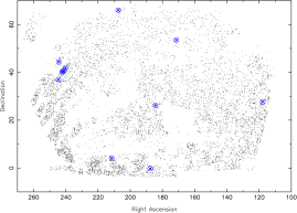
Figure 8: Projection of the moving group in equatorial coordinates, as detected in SDSS DR7. The small black dots show the positions of A stars with spectra that are not from SEGUE plates as selected from DR7. Only twelve of these stars (large cyan symbols) have surface gravities, metallicities, apparent magnitudes, and line-of-sight velocities that are consistent with the moving group, as detected in Figure 9. Of these twelve, four are very tightly clustered and a fifth is only a few degrees away and in line with the other four.

Figure 9: Detection of the moving group in SDSS DR7. This figure is similar to the upper right and lower left panels of Figure 1, with the additional restriction that the all the stars in these panels have $\rm[Fe/H]_{\rm WBG}<-1.95$. The significance of the group over background is enhanced with this metallicity cut.

The moving group was originally discovered by searching through data from SDSS DR6. In this section we show the moving group as selected from the now public SDSS DR7 databases, and using our knowledge of metallicity and surface gravity determination at low S/N, as learned in the production of this paper.

We selected from SDSS DR7 all of the spectra with elodierverr $>0$ (which selects stellar spectra), magnitude $15<g_{0}<23$, the colors of an A star [$0.8<(u-g)_{0}<1.5,-0.3<(g-r)_{0}<0.0$], and a flag that indicates the spectrum is not from a SEGUE plate. We did not select stars from SEGUE plates since most of them have not been searched for moving groups of A stars, and because their non-uniform sky coverage, different section criterion, and different exposure lengths make it difficult to use them in a statistical calculation. We show the distribution of SDSS DR7 A stars in equatorial coordinates in Figure 8.

We then selected the low surface gravity (logg9 $<3.0$) stars with $50^{\circ}<l<80^{\circ}$ and $40^{\circ}<b<55^{\circ}$, to match the region of the sky presented in Figure 1, and metallicity [Fe/H]${}_{\rm WBG}<-1.95$, since we know we are looking for a low metallicity moving group. Figure 9 shows plots like those used in the moving group discovery, but using data from this low metallicity DR7 dataset. From the upper panel, we identify a clump of stars with $-35<V_{gsr}<0.0$ km s^-1 and $18.8<g_{0}<18.9$. The lower panel shows the positions in Galactic coordinates of the same objects from the top panel, with filled circles showing the six objects that are clumped in line-of-sight velocity and apparent magnitude. Four of these objects are very tightly aligned in angular position on the sky.

To get a sense for how common a moving group with these characteristics is, we selected from our original DR7 dataset all of the stars with surface gravity, metallicity, line-of-sight velocity, and apparent magnitude that are similar to the stars in the clump. In the entire northern sky portion of the SDSS, there are twelve stars with these characteristics. Four of the stars are in a tight line on the sky, and a fifth is only a few degrees away from the clump along the same line. Because this fifth star is a candidate member of the moving group, and not included in the original list of seven, we have added it to the bottom of the list of candidate members in Table 1. The four highly probable members of the moving group, which were selected from both the DR6 and DR7 datasets, are marked in Table 1 with a footnote.

The four highly likely moving group members are a subset of the original seven, and have velocity and metallicity characteristics that are nearly identical to our previous results. The average $V_{gsr}$ is $-10\pm 3$ km s^-1, with a sigma of $6$ km s^-1. The average metallicity is [Fe/H]${}_{\rm WBG}=-2.4\pm 0.2$ with a sigma of 0.39.

Following a similar procedure to that used in Section 5, we now calculate the probability that this group of four stars is a random coincidence. There are 6118 stars with $b>35^{\circ}$ in the A star sample depicted in Figure 8. Of these stars, 3335 have $-9<{\rm logg9}<3.0$ (54.5%), 1171 have $-9<$ [Fe/H]${}_{\rm WBG}<-1.95$ (28.9%), 224 have $18.8<g_{0}<18.9$ (3.7%), and 487 have $-23<V_{gsr}<0$ km s^-1 (8.1%). The four stars in the clump have sky positions within $63.72^{\circ}<l<66.62^{\circ}$ (0.8% of longitude range) and $47.37^{\circ}<b<48.92^{\circ}$ (4.2% of area-corrected latitude range). Because the density of the stars in Figure 8 is not uniform, we need to use a multiplier on the fraction of stars in the longitude range, since that is fractionally the smallest dimension. In the 3.0 square degree area that contains the four stars, there are 8 stars in the original sample of 6118. So, in the region of the clump there are 2.7 stars per square degree, while there are $6118/8796=0.69$ stars per square degree in the whole sky region, a factor of 3.9. Using the procedure outlined in Appendix A, we calculate that we would expect 0.0038 stars in a 6-D region that instead has four stars. The expected number of clumps of four stars is 0.0238. The p-value is therefore less than 0.024 ($p<E=0.238$). Since $p<0.05$, this is a significant detection.

Note that this calculation is extremely conservative. First, the calculation assumed that we searched all 6118 stars for clumps, when in fact we only searched the ones that had low surface gravity, as determined by the photometric indices. Second, the four stars are not randomly distributed within the $(l,b)$ box, they are tightly constrained to a line, as one would expect for a tidally disrupted globular cluster; if our statistical analysis allowed a non-axis aligned region, the computed statistical significance would have been stronger. And third, when we calculated the density of stars in the region containing the moving group we included the moving group stars (half of the sample of eight) in the density calculation. This artificially inflates our Galactic latitude multiplier. To estimate the effect of just this third factor, we counted the number of A stars in a slightly larger region of the sky with $60^{\circ}<l<66.63^{\circ}$ and $47.37^{\circ}<b<48.92^{\circ}$ and found 16 stars, of which 4 are members of the moving group. This gives us a local density of $12/6.87=1.75$ stars per square degree, which is a factor of 2.5 times the average star density. Using this multiplier, we expect to find 0.0025 objects where we actually find four, and the expected fraction of the time a clump of four stars in this size region of 6-D space should be found in this size data set is not more than 0.0063.

9 Estimated luminosity of the progenitor

We estimate the properties of a progenitor of this moving group, making the assumption that it was a globular cluster, and that we have detected the majority of the BHB stars from what was the core of the star cluster. We expect the progenitor was a globular cluster because the stars are very well aligned in the sky, have a velocity dispersion consistent with instrumental errors, and there are very few stars identified. If the progenitor was a dwarf galaxy, so that it also has younger or more metal rich components, or if we have found only a knot of increased stellar density along a longer tidal debris stream, then the inferred size of the progenitor is larger.

We detected 4-8 BHB stars in the moving group. In the color-magnitude range in the vicinity of the moving group, we have spectra of 50 of the 73 candidate BHBs (68%). Therefore, we expect that there are $\sim 10$ BHBs in the moving group. Borissova et al. (1997) found five BHB stars in the globular cluster Pal 13 ([Fe/H]=$-1.74$, $M_{V}=-3.74$, Harris 1996). Yanny, Newberg et al. (2000) find at least five BHB stars in the globular cluster Pal 5 ([Fe/H]=$-1.41$, $M_{V}=-5.17$, Harris 1996). The moving group is consistent with a progenitor that is like one of the smaller globular clusters of the Milky Way, with a total integrated luminosity of about $M_{V}\sim-4$.

To understand why this moving group could not be identified from photometry alone, we estimated the number of red giant and subgiant branch stars in the moving group by comparison with NGC 2419. Note that at 50 kpc, turnoff stars are at $g_{0}\sim 22.7$, which is close to the limiting magnitude of the SDSS, so deeper photometry is required to clearly detect significant density enhancements expected from turnoff and main sequence stars fainter than these limits. We selected SDSS DR6 stars within about nine arcminutes of the centre of NGC 2419 (this does not include stars near the very centre of the GC, since individual stars are not resolved there). BHB stars were selected with $20.2<g_{0}<20.6$ and $-0.4<(g-r)_{0}<0.0$. Giant stars were selected within a parallelogram with vertices $[(g-r)_{0},g_{0}]=[0.5,20],[0.9,18],[0.7,20],[1.0,18]$. Subgiant stars were selected within a triangular area with vertices $[(g-r)_{0},g_{0}]=[0.5,21],[0.1,23],[0.6,23]$. We found 101 BHBs, 98 red giants, and 302 subgiants over background in the region of sky that was searched. Therefore, we expect about the same number of red giant stars as BHBs in our moving group, and about three times as many subgiants. We shifted the magnitudes of the color-magnitude boxes by 1.41 magnitudes (the difference in distance modulus between our moving group and NGC 2419) and counted the number of stars in $60^{\circ}<l<70^{\circ}$ and $45^{\circ}<b<50^{\circ}$. The moving group is expected to have 10 of 73 candidate BHB stars (1 sigma fluctuation), 10 of 2742 candidate giant stars (0.2 sigma), and 30 of 13,182 candidate subgiant stars (0.3 sigma). The background star counts are much too high for us to find this moving group in photometry alone.

10 Conclusions

We have detected a moving group of at least four BHB stars in the corner (“toe”) of the Hercules constellation spilling into Corona Borealis. These stars are coincident in angular position [$(l,b)=(65^{\circ},48^{\circ}$)], apparent magnitude ($g_{0}=18.9$), line-of-sight velocity ($V_{\mbox{\it gsr}}=-10$ km s^-1, $\sigma_{V_{\mbox{\it gsr}}}<10$ km s^-1, $\langle V_{r}\rangle=-157$ km s^-1), and metallicity ([Fe/H]=$-2.4$). We expect that the progenitor of this moving group was a low metallicity globular cluster, with a luminosity like that of one of the smaller globular clusters in the Milky Way halo.

We show that useful surface gravities and metallicities are measured for BHB stars with S/N$>7$ in SDSS DR7. The mean metallicity of BHB stars in the outer halo is similar to M53, which has a published metallicity of [Fe/H]=$-2.0$. The metallicity does not appear to change with distance from the Sun ($6<R<55$ kpc). Our measurement of the spheroid metallicity is slightly higher than claimed by Carollo et al. (2007) and somewhat lower than earlier studies of outer halo stars.

The Hercules moving group is one of many tidally disrupted stellar associations expected to comprise the spheroid of the Milky Way and could not have been identified from photometry alone; more complete spectroscopic surveys are required to identify the component spheroid moving groups, and determine the merger history of our galaxy. We present a statistical technique that allows us to estimate the significance of clumps discovered in multidimensional data.

Appendix A The Statistics of Clumpy Data

A.1 Introduction

For this paper, we needed to estimate the probability of finding seven BHB stars in a restricted portion of $l,b,V_{\mbox{\it gsr}},g_{0}$ parameter space. In this appendix, we present a solution to the more general problem of determining the probability of finding $K$ of $N$ data points in a small portion of a $d$-dimensional space.

Suppose one analyses of a set of $N$ data points in a large $d$-dimensional hypercube $[A_{1},B_{1}]\times\ldots\times[A_{d},B_{d}]$, and finds a small, axis-aligned, $d$-dimensional hypercube $[a_{1},b_{1}]\times\ldots\times[a_{d},b_{d}]$ that has $K\geq 2$ data points in it. The natural question is whether this “clump” of $K$ data points is statistically significant, or whether even random data would yield such a clump. Here we precisely estimate an $E$-value for the expected number of clumps, thus providing an upper bound to the probability that random data would somewhere have $K$ or more data points within an axis-aligned, $d$-dimensional hypercube with dimensions $(w_{1},\ldots,w_{d})=(b_{1}-a_{1},\ldots,b_{d}-a_{d})$.

A.2 Theory

We start with the simple case where a full data set of $N$ points lies within a $d$-dimensional unit hypercube $[0,1]^{d}$. We further assume that a random (or null) model would distribute these $N$ points uniformly within the hypercube. Additionally, we assume that the hypercube is not periodic/toroidal. We relax these simplifying assumptions in subsequent sections.

We say that an axis-aligned, $d$-dimensional hypercube contained within $[0,1]^{d}$ is a box. We say that a set of $K\geq 2$ of the $N$ points is a $K$-boxed set if there exists a box that contains the $K$ points without containing any of the remaining $N-K$ points. We define the minimal box for a $K$-boxed set as the intersection of all boxes that contain the $K$ points.

A box of dimensions $(w_{1},\ldots,w_{d})$ or smaller with $K$ or more points exists only if there is a $K$-boxed set that has a minimal box with dimensions not greater than $(w_{1},\ldots,w_{d})$. Thus, we aim to compute the expected number of the latter. We use as an integrand the probability density that a box will be a minimal box for a set of $K$ points, and we integrate over all applicable boxes.

Consider a box $[f_{1},g_{1}]\times\ldots\times[f_{d},g_{d}]$ with dimensions $(l_{1},\ldots,l_{d})=(f_{1}-g_{1},\ldots,f_{d}-g_{d})$ and hypervolume

$$V=\prod_{i=1}^{d}l_{i}\mbox{~{}.}$$ (1)

It will be a (non-minimal) box indicating that a set of $K$ points is a $K$-boxed set if exactly $K$ points fall within it. Thus the probability that it indicates a $K$-boxed set is

$$\left(\!\!\!\!\begin{array}[]{c}N\\ K\end{array}\!\!\!\!\right)V^{K}(1-V)^{N-K}\mbox{~{}.}$$ (2)

However, it is our goal to calculate the probability density for a minimal box for $K$ points. This box is minimal only if, for every dimension index $i$, we have that $f_{i}$ is the minimum of the $K$ points’ $i$th coordinate values and $g_{i}$ is the maximum of these coordinate values. Thus, for each dimension, we must have one of the $K$ points achieve the minimum and one of the remaining $K-1$ points achieve the maximum. The remaining $K-2$ coordinate values can be anywhere in the range $(f_{i},g_{i})$. (Note that the possibility of having multiple points exactly achieve the minimum or maximum is an event that has a probability density of zero and thus is safely ignored.) Thus, the $i$th dimension contributes a factor of $K(K-1){l_{i}}^{K-2}$ to the probability density. The probability density for the event that the box is a minimal box for a $K$-boxed set is

$$\Pr[K|l_{1},\ldots,l_{d}]=\left(\!\!\!\!\begin{array}[]{c}N\\ K\end{array}\!\!\!\!\right)K^{d}(K-1)^{d}V^{K-2}(1-V)^{N-K}\mbox{~{}.}$$ (3)

We note that a box with dimensions $(l_{1},\ldots,l_{d})$ can have its minimum corner $(f_{1},\ldots,f_{d})$ anywhere in $[0,1-l_{1}]\times\ldots\times[0,1-l_{d}]$. When we restrict attention to minimal boxes with dimensions not greater than $(w_{1},\ldots,w_{d})$ the expected number of $K$-boxed sets is

$$E(K,w_{1},\ldots,w_{d})=$$ (4)

$$\int_{0}^{w_{1}}dl_{1}\ldots\int_{0}^{w_{d}}dl_{d}\left(\prod_{i=1}^{d}(1-l_{i})\right)\Pr[K|l_{1},\ldots,l_{d}].\mbox{~{}.}$$

Equation 4 provides an upper bound to the probability that random data will exhibit a clump of $K$ or more points in a box of dimensions $(w_{1},\ldots,w_{d})$ or smaller, because such a box exists only if there is a $K$-boxed set that has a minimal box with dimensions not greater than $(w_{1},\ldots,w_{d})$. Under many circumstances, when $E\ll 1$ the probability of multiple $K$-boxed sets is small and the bound is quite tight.

A.3 Implementation

We observe that

$$(1-V)^{N-K}=\sum_{m=0}^{N-K}\left(\!\!\!\!\begin{array}[]{c}N-K\\ m\end{array}\!\!\!\!\right)(-V)^{m}\mbox{~{},}$$ (5)

and, to speed the integration using Maple 7, we seek a way to truncate the sum at significantly fewer terms. We observe that $\left(\!\!\!\!\begin{array}[]{c}N-K\\ m\end{array}\!\!\!\!\right)V^{m}$ is roughly a bell curve as a function of $m$. The bell curve has mean and standard deviation given by

$$\mu = \frac{(N-K)V}{1+V}\leq NV\leq K$$ (6)

$$\sigma = \sqrt{\frac{(N-K)V}{(1+V)^{2}}}\leq\sqrt{NV}\leq\sqrt{K}\mbox{~{},}$$ (7)

where we have assumed that $K\geq NV$, i.e., that a clump is under consideration only when the number of points it contains is more than the expected number.

Thus, we can include all terms of $(1-V)^{N-K}$ out to $z=10$ standard deviations with $m^{*}=\max(\lceil\mu+z\sigma\rceil,25)$ and the precise approximation

$$(1-V)^{N-K}\approx\sum_{m=0}^{m^{*}}\left(\!\!\!\!\begin{array}[]{c}N-K\\ m\end{array}\!\!\!\!\right)(-V)^{m}\mbox{~{}.}$$ (8)

We use this approximation in Equation 4 and we evaluate the integral with Maple 7.

A.4 Variations

A.4.1 Non-Unit Hypercubes and Non-Uniform Random Distributions

In many circumstances, including the case presented in this paper, the set of $N$ data points does not fall uniformly into the unit hypercube under the random/null model. For instance, one does not expect the radial velocities of spheroid stars to be uniformly distributed in any velocity range, and they are certainly not limited to the range $[0,1]$.

We say that the density is separable if it can be written as the product of functions, each of which depends on a single dimension $\Pr(\vec{x})\propto\prod_{i=1}^{d}h_{i}(x_{i})$. For instance, the uniform spherical density,

$$\Pr(r,\theta,\phi)=\frac{1}{4\pi R^{3}/3}r^{2}\sin(\theta)\,dr\,d\theta\,d\phi\mbox{~{}.}$$ (9)

is separable. When a probability density for a coordinate vector $\vec{x}\in[A_{i},B_{i}]\times\ldots\times[A_{d},B_{d}]$ is separable, we can perform a coordinate transformation to a coordinate vector $\vec{y}$ that is uniformly distributed in the unit hypercube and which preserves axis-aligned hypercubes:

$$y_{i}=\frac{\int_{A_{i}}^{x_{i}}h_{i}(x^{\prime}_{i})\,dx^{\prime}_{i}}{\int_{A_{i}}^{B_{i}}h_{i}(x^{\prime}_{i})\,dx^{\prime}_{i}}\mbox{~{}.}$$ (10)

The clumping question then becomes one of percentiles, i.e., what is the probability that random data will show $K$ or more points in a axis-aligned hypercube with dimensions that do not exceed $w_{i}$ percentiles $\times\ldots\times w_{d}$ percentiles. In this paper, the radial velocities of the stars and the apparent $g_{0}$ magnitudes were treated as separable dimensions.

A.4.2 Periodic or Toroidal Boundary Conditions

In many circumstances, it is desirable to allow $K$-boxed sets to wrap around the boundaries in one or more dimensions. In this paper, it was desirable to allow a box to span the prime meridian in a longitude coordinate. In such situations the restriction that the minimum corner $(f_{1},\ldots,f_{d})$ fall in $[0,1-l_{1}]\times\ldots\times[0,1-l_{d}]$ is relaxed. When the $i$th coordinate is periodic, $f_{i}$ can be any value in $[0,1]$. Equation 4 is thus modified by removal of the $(1-l_{i})$ factor for each periodic dimension $i$.

A.4.3 Poisson Distributions

In many circumstances, it is desirable to have the random/null model be Poisson; instead of requiring exactly $N$ points in the unit hypercube, the number of points $n$ is selected using a Poisson distribution with mean $N$:

$$\Pr[n|N]=e^{-N}\frac{N^{n}}{n!}\mbox{~{}.}$$ (11)

In our example, the Poisson distribution applies if there are an average of 4149 BHB stars with spectra in the region $b>45^{\circ}$, whereas the uniformly random model would put exactly 4149 BHB stars with spectra in that same region.

In the Poisson case, Expression 2 becomes

$$\frac{N^{K}}{K!}V^{K}e^{-NV}\mbox{~{},}$$ (12)

Equation 3 becomes

$$\Pr[K|l_{1},\ldots,l_{d}]=\frac{N^{K}}{K!}K^{d}(K-1)^{d}V^{K-2}e^{-NV}\mbox{~{},}$$ (13)

and Equation 4 is unmodified, except that it incorporates Equation 13 instead of Equation 3.

For integration, instead of truncating the series for $(1-V)^{N-K}$, we truncate the series for

$$e^{-NV}=\sum_{m=0}^{\infty}\frac{(-NV)^{m}}{m!}\mbox{~{}.}$$ (14)

We observe that $(NV)^{m}/m!$ is roughly a bell curve as a function of $m$. The bell curve has mean and standard deviation given by

$$\mu = NV\leq K$$ (15)

$$\sigma = \sqrt{NV}\leq\sqrt{K}\mbox{~{}.}$$ (16)

Thus, we can include all terms of $\exp(-NV)$ out to $z$ standard deviations with $m^{*}=\max(\lceil\mu+z\sigma\rceil,25)$ and the precise approximation

$$e^{-NV}\approx\sum_{m=0}^{m^{*}}\frac{(-NV)^{m}}{m!}\mbox{~{}.}$$ (17)

We use this approximation in Equation 13 and we evaluate the integral of Equation 4 with Maple 7. We determined that for this paper the distinction between random and Poisson distributions was unimportant.

A.4.4 Non-Separability

When the dimensions are not separable, the assumption that the joint density function is the product of the individual dimension’s density functions does not hold. However, if there is a set of individual density functions for which the assumption is approximately true, we define the overdensity to be the ratio of joint density function to the value implied by multiplying the approximating density functions together. The calculations for the separable case make a good approximation for the non-separable case if the percentile widths $(w_{1},\ldots,w_{d})$ are adjusted by factors whose product is the overdensity. When the overdensity is greater than 1.0, a conservative approach is to multiply the smallest of the widths of the non-separable dimensions by the overdensity.

References

- Abazajian et al. (2003) Abazajian K. et al., 2003, AJ, 126, 2081
- Adelman-McCarthy et al. (2008) Adelman-McCarthy J. K. et al., 2008, ApJS, 175, 297
- Allende Prieto et al. (2006) Allende Prieto, C. et al. 2006, ApJ, 636, 804
- An et al. (2009) An, D., et al. 2009, ApJL, 707, L64
- Belokurov et al. (2009) Belokurov, V., et al. 2009, MNRAS, 397, 1748
- Belokurov et al. (2007) Belokurov V. et al., 2007, ApJL, 657, L89
- Belokurov et al. (2007) Belokurov V. et al., 2007, ApJ, 654, 897
- Belokurov et al. (2006) Belokurov V. et al., 2006, ApJL, 647, L111
- Belokurov et al. (2006) Belokurov V. et al., 2006, ApJL, 642, L137
- Boc (1934) Bok B. J., 1934, Harvard College Observatory Circular, 384, 1
- Borissova et al. (1997) Borissova J., Markov H., & Spassova N., 1997, A&AS, 121, 499
- Carney et al. (1990) Carney B. W., Aguilar L., Latham D. W., & Laird J. B., 1990, AJ, 99, 201
- Carollo et al. (2010) Carollo, D. et al. 2010, ApJ, in press, arXiv:0909.3019
- Carollo et al. (2007) Carollo D. et al., 2007, Nature, 450, 1020
- Clewley & Kinman (2006) Clewley L., & Kinman T. D., 2006, MNRAS, 371, L11
- Dehnen & Binney (1998) Dehnen W. & Binney J.J., 1998, MNRAS, 298, 387
- Eggen (1958) Eggen O. J., 1958, MNRAS, 118, 65
- Famaey et al. (2008) Famaey B., Siebert A., & Jorissen A., 2008, A&A, 483, 453
- Freeman (1987) Freeman K. C., 1987, ARA&A, 25, 603
- Fukugita et al. (1996) Fukugita M., Ichikawa T., Gunn J. E., Doi M., Shimasaku K., & Schneider D. P., 1996, AJ, 111, 1748
- Gilmore, Wyse, & Kuijken (1989) Gilmore G., Wyse R. F. G. & Kuijken K., 1989, ARA&A 27, 555
- Grillmair (2006) Grillmair C. J., 2006, ApJL, 645, L37
- Grillmair & Dionatos (2006) Grillmair C. J., & Dionatos O., 2006, ApJL, 643, L17
- Grillmair & Johnson (2006) Grillmair C. J., & Johnson R., 2006, ApJL, 639, L17
- Gunn et al. (1998) Gunn J. E. et al., 1998, AJ, 116, 3040
- Gunn et al. (2006) Gunn J. E. et al., 2006, AJ, 131, 2332
- Harris (1996) Harris W. E., 1996, AJ, 112, 1487
- Helmi et al. (2003) Helmi A., White S. D. M., & Springel V., 2003, MNRAS, 339, 834
- Hogg et al. (2001) Hogg D.W., Finkbeiner D.P., Schlegel D.J., & Gunn J.E., 2001, AJ, 122, 2129
- Irwin et al. (2007) Irwin M. J. et al., 2007, ApJL, 656, L13
- Ivezić et al. (2004) Ivezić Ž. et al., 2004, Astronomische Nachrichten, 325, 583
- Jurić et al. (2008) Jurić M. et al., 2008, ApJ, 673, 864
- Koposov et al. (2009) Koposov S. E., Yoo J., Rix H.-W., Weinberg D. H., Macciò A. V., & Escudé J. M., 2009, ApJ, 696, 2179
- Klement et al. (2009) Klement, R., et al. 2009, ApJ, 698, 865
- Kurucz (1993) Kurucz, R. L. 1993, Kurucz CD-ROM 13, ATLAS9 Stellar Atmosphere Programs and 2 km/s grid (Cambridge, MA: SAO)
- Lee et al. (2008b) Lee, Y. S. et al. 2008, AJ, 136, 2050
- Lee et al. (2008a) Lee, Y. S. et al. 2008, AJ, 136, 2022
- Majewski et al. (2003) Majewski S. R., Skrutskie M. F., Weinberg M. D., & Ostheimer J. C., 2003, ApJ, 599, 1082
- Majewski et al. (2004) Majewski S. R., Ostheimer J. C., Rocha-Pinto H. J., Patterson R. J., Guhathakurta P., & Reitzel D., 2004, ApJ, 615, 738
- Majewski et al. (1996) Majewski S. R., Munn J. A. & Hawley S. L., 1996, ApJL, 459, L73
- Morrison et al. (2003) Morrison H. L. et al., 2003, AJ, 125, 2502
- Newberg et al. (2009) Newberg, H. J., Yanny, B., & Willett, B. A. 2009, ApJL, 700, L61
- Newberg et al. (2007) Newberg, H. J., Yanny, B., Cole, N., Beers, T. C., Re Fiorentin, P., Schneider, D. P., & Wilhelm, R. 2007, ApJ, 668, 221
- Newberg & Yanny (2005) Newberg H. J., & Yanny B., 2005, Astrometry in the Age of the Next Generation of Large Telescopes, ASP Conf. Ser., 338, 210
- Newberg et al. (2002) Newberg H. J. et al., 2002, ApJ, 569, 245
- Norris (1986) Norris J., 1986, ApJS, 61, 667
- Odenkirchen et al. (2003) Odenkirchen M. et al., 2003, AJ, 126, 2385
- Padmanabhan et al. (2008) Padmanabhan N. et al., 2008, ApJ, 674, 1217
- Pier et al. (2003) Pier J. R., Munn J. A., Hindsley R. B., Hennessy G. S., Kent S. M., Lupton R. H., & Ivezić Ž., 2003, AJ, 125, 1559
- Pier (1983) Pier, J. R. 1983, ApJS, 53, 791
- Robin et al. (2000) Robin A. C., Reylé C., & Crézé M., 2000, A&A, 359, 103
- Saha (1985) Saha A., 1985, ApJ, 289, 310
- Schlaufman et al. (2009) Schlaufman K. C. et al., 2009, ApJ, in preparation
- Schlegel et al. (1998) Schlegel D. J., Finkbeiner D. P., & Davis M., 1998, ApJ, 500, 525
- Searle & Zinn (1978) Searle L., & Zinn R., 1978, ApJ, 225, 357
- Sirko et al. (2004) Sirko E. et al., 2004, AJ, 127, 899
- Smith et al. (2009) Smith, M. C., et al. 2009, MNRAS, 399, 1223
- Smith et al. (2002) Smith J. A. et al., 2002, AJ, 123, 2121
- Stoughton et al. (2002) Stoughton C. et al., 2002, AJ, 123, 485
- Suntzeff et al. (1991) Suntzeff N. B., Kinman T. D., & Kraft R. P., 1991, ApJ, 367, 528
- Tucker et al. (2006) Tucker D. L. et al., 2006, Astronomische Nachrichten, 327, 821
- Vivas et al. (2001) Vivas A. K. et al., 2001, ApJL, 554, L33
- Walsh, Jerjen, & Willman (2007) Walsh, S. M., Jerjen, H., & Willman, B. 2007, ApJL, 662, L83
- Wilhelm, Beers, & Gray (1999) Wilhelm R., Beers T. C., & Gray R. O., 1999, AJ, 117, 2308 (WBG).
- Willman et al. (2005b) Willman B. et al., 2005, ApJL, 626, L85
- Willman et al. (2005a) Willman B. et al., 2005, AJ, 129, 2692
- Xue et al. (2008) Xue, X. X., et al. 2008, ApJ, 684, 1143
- Yanny et al. (2009) Yanny B. et al., 2009, AJ, 137, 4377
- Yanny et al. (2003) Yanny B. et al., 2003, ApJ, 588, 824
- Yanny, Newberg et al. (2000) Yanny B., Newberg H. J., et al., 2000, ApJ, 540, 825
- York et al. (2000) York D. G. et al., 2000, AJ, 120, 1579
- Zinn (1985) Zinn R., 1985, ApJ, 293, 424
- Zucker et al. (2006b) Zucker D. B. et al., 2006, ApJL, 650, L41
- Zucker et al. (2006a) Zucker D. B. et al., 2006, ApJL, 643, L103