Privacy-Preserving Protocols
for Eigenvector Computation

Abstract

In this paper, we present a protocol for computing the principal eigenvector of a collection of data matrices belonging to multiple semi-honest parties with privacy constraints. Our proposed protocol is based on secure multi-party computation with a semi-honest arbitrator who deals with data encrypted by the other parties using an additive homomorphic cryptosystem. We augment the protocol with randomization and obfuscation to make it difficult for any party to estimate properties of the data belonging to other parties from the intermediate steps. The previous approaches towards this problem were based on expensive QR decomposition of correlation matrices, we present an efficient algorithm using the power iteration method. We analyze the protocol for correctness, security, and efficiency.

1 Introduction

Eigenvector computation is one of the most basic tools of data analysis. In any multivariate dataset, the eigenvectors provide information about key trends in the data, as well as the relative importance of the different variables. These find use in a diverse set of applications, including principal component analysis [7], collaborative filtering [4] and PageRank [8]. Not all eigenvectors of the data are equally important; only those corresponding to the highest eigenvalues are used as representations of trends in the data. The most important eigenvector is the principal eigenvector corresponding to the maximum eigenvalue.

In many scenarios, the entity that actually computes the eigenvectors is different from the entities that possess the data. For instance, a data mining agency may desire to compute the eigenvectors of a distributed set of records, or an enterprise providing recommendations may want to compute eigenvectors from the personal ratings of subscribers to facilitate making recommendations to new customers. We will refer to such entities as arbitrators. Computation of eigenvectors requires the knowledge of either the data from the individual parties or the correlation matrix derived from it. The parties that hold the data may however consider them private and be unwilling to expose any aspect of their individual data to either the arbitrator or to other parties, while being agreeable, in principle, to contribute to the computation of a global trend. As a result, we require a privacy preserving algorithm that can compute the eigenvectors of the aggregate data while maintaining the necessary privacy of the individual data providers.

The common approach to this type of problem is to obfuscate individual data through controlled randomization [3]. However, since we desire our estimates to be exact, simple randomization methods that merely ensure accuracy in the mean cannot be employed. Han, et al. [6] address the problem by computing the complete QR decomposition [5] of privately shared data using cryptographic primitives. This enables all parties to collaboratively compute the complete set of global eigenvectors but does not truly hide the data from individual sources. Given the complete set of eigenvectors and eigenvalues provided by the QR decomposition, any party can reverse engineer the correlation matrix for the data from the remaining parties and compute trends among them. Canny [2] present a different distributed approach that does employ an arbitrator, in their case a blackboard, however although individual data instances are hidden, both the arbitrator and individual parties have access to all aggregated individual stages of the computation and the final result is public, which is much less stringent than our privacy constraints.

In this paper, we propose a new privacy-preserving protocol for shared computation of the principal eigenvector of a distributed collection of privately held data. The algorithm is designed such that the individual parties, whom we will refer to as “Alice” and “Bob” learn nothing about each others’ data, and only learn the degree to which their own data follow the global trend indicated by the principal eigenvector. The arbitrator, who we call “Trent”, coordinates the computation but learns nothing about the data of the individual parties besides the principal eigenvector which he receives at the end of the computation. In our presentation, for simplicity, we initially consider two parties each having an individual data matrix. Later we show that the protocol can be naturally generalized to $N$ parties. As the $N$ parties communicate only with Trent in a star network topology with $O(N)$ data transmissions, this is much more efficient than the $O(N^{2})$ data transmission cost if all parties communicated with each other in a fully connected network. The data may be split in two possible ways: along data instances or features. In this work, we principally consider the data-split case. However, our algorithm is easily applied to feature split data as well.

We use the power iteration method [5] to compute the principal eigenvector. The arbitrator Trent introduces a combination of homomorphic encryption [9], randomization, and obfuscation to ensure that the computation preserves privacy. The algorithm assumes the parties to be semi-honest. While they are assumed to follow the protocol correctly and refrain from using falsified data as input, they may record and analyze the intermediate results obtained while following the protocol in order to to gain as much information as possible. It is required that no party colludes with Trent as this will compromise the privacy of the protocol.

The computational requirements of the algorithm are the same as that of the power iteration method. In addition, each iteration requires the encryption and decryption of two $k$ dimensional vectors, where $k$ is the dimensionality of the data, as well as transmission of the encrypted vectors to and from Trent. Nevertheless, the encryption and transmission overhead, which is linear in $k$, may be expected to be significantly lower than the calculating the QR decomposition or similar methods which require repeated transmission of entire matrices. In general, the computational cost of the protocol is dependent on the degree of security we desire as required by the application.

2 Preliminaries

2.1 Power Iteration Method

The power iteration method [5] is an algorithm to find the principal eigenvector and its associated eigenvalue for square matrices. To simplify explanation, we assume that the matrix is diagonalizable with real eigenvalues, although the algorithm is applicable to general square matrices as well [11]. Let $A$ be a size $N\times N$ matrix whose eigenvalues are $\lambda_{1},\ldots,\lambda_{N}$.

The power iteration method computes the principal eigenvector of $A$ through the iteration

$$x_{n+1}\leftarrow\frac{Ax_{n}}{\|Ax_{n}\|},$$

where $x_{n}$ is a $N$ dimensional vector. If the principal eigenvalue is unique, the series $\omega_{n}=A^{n}x_{0}$ is guaranteed to converge to a scaling of the principal eigenvector. In the standard algorithm, $\ell_{2}$ normalization is used to prevent the magnitude of the vector from overflow and underflow. Other normalization factors can also be used if they do not change the limit of the series.

We assume wlog that $|\lambda_{1}|\geq\cdots\geq|\lambda_{N}|\geq 0$. Let $v_{i}$ be the normalized eigenvector corresponding to $\lambda_{i}$. Since $A$ is assumed to be diagonalizable, the eigenvectors $\{v_{1},\ldots,v_{N}\}$ create a basis for $\mathbb{R}^{N}$. For unique values of $c_{i}\in\mathbb{R}^{N}$, any vector $x_{0}\in\mathbb{R}^{N}$ can be written as $x_{0}=\sum_{i=1}^{N}c_{i}v_{i}$. It can be shown that $\frac{1}{|\lambda_{1}|^{n}}A^{n}x_{0}$ is asymptotically equal to $c_{1}v_{1}$ which forms the basis of the power iteration method and the convergence rate of the algorithm is $\left|\frac{\lambda_{2}}{\lambda_{1}}\right|$. The algorithm converges quickly when there is no eigenvalue close in magnitude to the principal eigenvalue.

2.2 Homomorphic Encryption

A homomorphic encryption algorithm allows for operations to be perform on the encrypted data without requiring to know the unencrypted values. If $\cdot$ and $+$ are two operators and $x$ and $y$ are two plaintext elements, a homomorphic encryption function $E$ satisfies

$$E[x]\cdot E[y]=E[x+y].$$

In this work, we use the additive homomorphic Paillier asymmetric key cryptosystem [9].

3 Privacy Preserving Protocol

3.1 Data Setup and Privacy Requirements

We formally define the problem, in which multiple parties, try to compute the principal eigenvector over their collectively held datasets without disclosing any information to each other. For simplicity, we describe the problem with two parties, Alice and Bob; and later show that the algorithm is easily extended to multiple parties.

The parties Alice and Bob are assumed to be semi-honest which means that the parties will follow the steps of the protocol correctly and will not try to cheat by passing falsified data aimed at extracting information about other parties. The parties are assumed to be curious in the sense that they may record the outcomes of all intermediate steps of the protocol to extract any possible information. The protocol is coordinated by the semi-honest arbitrator Trent. Alice and Bob communicate directly with Trent rather than each other. Trent performs all the intermediate computations and transfers the results to each party. Although Trent is trusted not to collude with other parties, it is important to note that the parties do not trust Trent with their data and intend to prevent him from being able to see it. Alice and Bob hide information by using a shared key cryptosystem to send only encrypted data to Trent.

We assume that both the datasets can be represented as matrices in which columns and rows correspond to the data samples and the features, respectively. For instance, the individual email collections of Alice and Bob are represented as matrices $A$ and $B$ respectively, in which the columns correspond to the emails, and the rows correspond to the words. The entries of these matrices represent the frequency of occurrence of a given word in a given email. The combined dataset may be split between Alice and Bob in two possible ways. In a data split, both Alice and Bob have a disjoint set of data samples with the same features. The aggregate dataset is obtained by concatenating columns given by the data matrix $M=\begin{bmatrix}A&B\end{bmatrix}$ and correlation matrix $M^{T}M$. In a feature split, Alice and Bob have different features of the same data. The aggregate data matrix $M$ is obtained by concatenating rows given by the data matrix $M=\begin{bmatrix}A\\ B\end{bmatrix}$ and correlation matrix $MM^{T}$. If $v$ is an eigenvector of $M^{T}M$ with a non-zero eigenvalue $\lambda$, we have

$$M^{T}Mv=\lambda v~{}\Rightarrow~{}MM^{T}Mv=\lambda Mv.$$

Therefore, $Mv\neq 0$ is the eigenvector of $MM^{T}$ with eigenvalue $\lambda$. Similarly, any eigenvector of horizontally split data $MM^{T}$ associated with a non-zero eigenvalue is an eigenvector of vertically split data $M^{T}M$ corresponding to the same eigenvalue. Hence, we mainly deal with calculating the principal eigenvector of the vertically split data. In practice the correlation matrix that has the smaller size should be used to reduce the computational cost of eigen-decomposition algorithms.

For vertical data split, if Alice’s data $A$ is of size $k\times m$ and Bob’s data $B$ is of size $k\times n$, the combined data matrix will be $M_{k\times(m+n)}$. The correlation matrix of size $(m+n)\times(m+n)$ is given by

$$M^{T}M=\begin{bmatrix}A^{T}A~{}&~{}A^{T}B\\ B^{T}A~{}&~{}B^{T}B\end{bmatrix}.$$

3.2 The Basic Protocol

The power iteration algorithm computes the principal eigenvector of $M^{T}M$ by updating and normalizing the vector $x_{t}$ until convergence. Starting with a random vector $x_{0}$, we calculate

$$x_{i+1}=\frac{M^{T}M~{}x_{i}}{\|M^{T}M~{}x_{i}\|}.$$

For privacy, we split the vector $x_{i}$ into two parts, $\alpha_{i}$ and $\beta_{i}$. $\alpha_{i}$ corresponds to the first $m$ components of $x_{i}$ and $\beta_{i}$ corresponds to the remaining $n$ components. In each iteration, we need to securely compute

$$M^{T}Mx_{i} =\begin{bmatrix}A^{T}A~{}&~{}A^{T}B\\ B^{T}A~{}&~{}B^{T}B\end{bmatrix}\begin{bmatrix}\alpha_{i}\\ \beta_{i}\end{bmatrix}=\begin{bmatrix}A^{T}(A\alpha_{i}+B\beta_{i})\\ B^{T}(A\alpha_{i}+B\beta_{i})\end{bmatrix}=\begin{bmatrix}A^{T}u_{i}\\ B^{T}u_{i}\end{bmatrix}$$ (1)

where $u_{i}=A\alpha_{i}+B\beta_{i}.$ After convergence, $\alpha_{i}$ and $\beta_{i}$ will represent shares held by Alice and Bob of the principal eigenvector of $M^{T}M$.

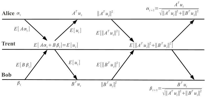
Figure 1: Visual description of the protocol.

This now lays the groundwork for us to define a distributed protocol in which Alice and Bob work only on their portions of the data, while computing the principal eigenvector of the combined data in collaboration with a third party Trent. An iteration of the algorithm proceeds as illustrated in Fig. 1. At the outset Alice and Bob randomly generate component vectors $\alpha_{0}$ and $\beta_{0}$ respectively. At the beginning of the $i^{\rm th}$ iteration, Alice and Bob possess component vectors $\alpha_{i}$ and $\beta_{i}$ respectively. They compute the product of their data and their corresponding component vectors as $A\alpha_{i}$ and $B\beta_{i}$. To compute $u_{i}$, Alice and Bob individually transfer these products to Trent. Trent adds the contributions from Alice and Bob by computing

$$u_{i}=A\alpha_{i}+B\beta_{i}.$$

He then transfers $u_{i}$ back to Alice and Bob, who then individually compute $A^{T}u_{i}$ and $B^{T}u_{i}$, without requiring data from one other. For normalization, Alice and Bob also need to securely compute the term

$$\|M^{T}M~{}x_{i}\|=\sqrt{\|A^{T}u_{i}\|^{2}+\|B^{T}u_{i}\|^{2}}.$$ (2)

Again, Alice and Bob compute the individual terms $\|A^{T}u_{i}\|^{2}$ and $\|B^{T}u_{i}\|^{2}$ respectively and transfer it to Trent. As earlier, Trent computes the sum

$$\|A^{T}u_{i}\|^{2}+\|B^{T}u_{i}\|^{2}$$

and transfers it back to Alice and Bob. Finally, Alice and Bob respectively update $\alpha$ and $\beta$ vectors as

$$u_{i}=A\alpha_{i}+B\beta_{i},$$

$$\alpha_{i+1}=\frac{A^{T}u_{i}}{\sqrt{\|A^{T}u_{i}\|^{2}+\|B^{T}u_{i}\|^{2}}},$$

$$\beta_{i+1}=\frac{B^{T}u_{i}}{\sqrt{\|A^{T}u_{i}\|^{2}+\|B^{T}u_{i}\|^{2}}}.$$ (3)

The algorithm terminates when the $\alpha$ and $\beta$ vectors converge.

3.3 Making the Protocol More Secure

The basic protocol described above is provably correct. After convergence, Alice and Bob end up with the principal eigenvector of the row space of the combined data, as well as concatenative shares of the column space which Trent can gather to compute the principal eigenvector. However the protocol is not secure; Alice and Bob obtain sufficient information about properties of each others’ data matrices, such as their column spaces, null spaces, and correlation matrices. We present a series of modifications to the basic protocol so that such information is not revealed.

3.3.1 Homomorphic Encryption: Securing the data from Trent.

The central objective of the protocol is to prevent Trent from learning anything about either the individual data sets or the combined data other than the principal eigenvector of the combined data. Trent receives a series of partial results of the form $AA^{T}u$, $BB^{T}u$ and $MM^{T}u$. By analyzing these results, he can potentially determine the entire column spaces of Alice and Bob as well as the combined data. To prevent this, we employ an additive homomorphic cryptosystem introduced in Section 2.2.

At the beginning of the protocol, Alice and Bob obtain a shared public key/private key pair for an additive homomorphic cryptosystem from an authenticating authority. The public key is also known to Trent who, however, does not know the private key; While he can encrypt data, he cannot decrypt it. Alice and Bob encrypt all transmissions to Trent, at the first transmission step of each iteration Trent receives the encrypted inputs $E[A\alpha_{i}]$ and $E[B\beta_{i}]$. He multiplies the two element by element to compute $E[A\alpha_{i}]\cdot E[B\beta_{i}]=E[A\alpha_{i}+B\beta_{i}]=E[u_{i}]$. He returns $E[u_{i}]$ to both Alice and Bob who decrypt it with their private key to obtain $u_{i}$. In the second transmission step of each iteration, Alice and Bob send $E[\|A^{T}u_{i}\|^{2}]$ and $E[\|B^{T}u_{i}\|^{2}]$ respectively to Trent, who computes the encrypted sum

$$E\left[\|A^{T}u_{i}\|^{2}\right]\cdot E\left[\|B^{T}u_{i}\|^{2}\right]=E\left[\|A^{T}u_{i}\|^{2}+\|B^{T}u_{i}\|^{2}\right]$$

and transfers it back to Alice and Bob, who then decrypt it to obtain $\|A^{T}u_{i}\|^{2}+\|B^{T}u_{i}\|^{2}$, which is required for normalization.

This modification does not change the actual computation of the power iterations in any manner. Thus the procedure remains as correct as before, except that Trent now no longer has any access to any of the intermediate computations. At the termination of the algorithm he can now receive the converged values of $\alpha$ and $\beta$ from Alice and Bob, who will send it in clear text.

3.3.2 Random Scaling: Securing the Column Spaces.

After Alice and Bob receive $u_{i}=A\alpha_{i}+B\beta_{i}$ from Trent, Alice can calculate $u_{i}-A\alpha_{i}=B\beta_{i}$ and Bob can calculate $u_{i}-B\beta_{i}=A\alpha_{i}$. After a sufficient number of iterations, particularly in the early stages of the computation (when $u_{i}$ has not yet converged) Alice can find the column space of $B$ and Bob can find the column space of $A$. Similarly, by subtracting their share from the normalization term returned by Trent, Alice and Bob are able to find $\|B^{T}u_{i}\|^{2}$ and $\|A^{T}u_{i}\|^{2}$ respectively.

In order to prevent this, Trent multiplies $u_{i}$ with a randomly generated scaling term $r_{i}$ that he does not share with anyone. Trent computes

$$\left(E[A\alpha_{i}]\cdot E[B\beta_{i}]\right)^{r_{i}}=E[r_{i}(A\alpha_{i}+B\beta_{i})]=E[r_{i}u_{i}]$$

by performing element-wise exponentiation of the encrypted vector by $r_{i}$ and transfers $r_{i}u_{i}$ to Alice and Bob. By using a different value of $r_{i}$ at each iteration, Trent ensures that Alice and Bob are not able to calculate $B\beta_{i}$ and $A\alpha_{i}$ respectively. In the second step, Trent scales the normalization constant by $r_{i}^{2}$,

$$\left(E\left[\|A^{T}u_{i}\|^{2}\right]\cdot E\left[\|B^{T}u_{i}\|^{2}\right]\right)^{r_{i}^{2}}=E\left[r_{i}^{2}\left(\|A_{i}^{T}u\|^{2}+\|B_{i}^{T}u\|^{2}\right)\right].$$

Normalization causes the $r_{i}$ factor to cancel out and the update rules remain unchanged.

$$u_{i}=A\alpha_{i}+B\beta_{i},$$

$$\alpha_{i+1}=\frac{r_{i}A^{T}u_{i}}{\sqrt{r_{i}^{2}\left(\|A^{T}u_{i}\|^{2}+\|B^{T}u_{i}\|^{2}\right)}}=\frac{A^{T}u_{i}}{\sqrt{\|A^{T}u_{i}\|^{2}+\|B^{T}u_{i}\|^{2}}},$$

$$\beta_{i+1}=\frac{r_{i}B^{T}u_{i}}{\sqrt{r_{i}^{2}\left(\|A^{T}u_{i}\|^{2}+\|B^{T}u_{i}\|^{2}\right)}}=\frac{B^{T}u_{i}}{\sqrt{\|A^{T}u_{i}\|^{2}+\|B^{T}u_{i}\|^{2}}}.$$ (4)

The random scaling does not affect the final outcome of the computation, and the algorithm remains correct as before.

3.3.3 Data Padding: Securing null spaces.

In each iteration, Alice observes one vector $r_{i}u_{i}=r_{i}(A\alpha_{i}+B\beta_{i})$ in the column space of $M=[A~{}B]$. Alice can calculate the null space $H(A)$ of $A$, given by

$$H(A)=\{x\in\mathbb{R}^{m}|Ax=0\}$$

and pre-multiply a non-zero vector $x\in H(A)$ with $r_{i}u_{i}$ to calculate

$$xr_{i}u_{i}=r_{i}x(A\alpha_{i}+B\beta_{i})=r_{i}xB\beta_{i}.$$

This is a projection of $B\beta_{i}$, a vector in the column space of $B$ into the null space $H(A)$. Similarly, Bob can find projections of $A\alpha_{i}$ in the null space $H(B)$. While considering the projected vectors separately will not give away much information, after several iterations Alice will have a projection of the column space of $B$ on the null space of $A$, thereby learning about the component’s of Bob’s data that lie in her null space. Bob can similarly learn about the component’s of Alice’s data that lie in his null space.

In order to prevent this, Alice participates in the protocol with a padded matrix $\begin{bmatrix}A&P_{a}\end{bmatrix}$ as input created by concatenating her data matrix $A$ with a random matrix $P_{a}=r_{a}I_{k\times k}$, where $r_{a}$ is a positive scalar chosen by Alice. Similarly, Bob uses a padded matrix $\begin{bmatrix}B&P_{b}\end{bmatrix}$ created by concatenating his data matrix $B$ with $P_{b}=r_{b}I_{k\times k}$, where $r_{b}$ is a different positive scalar chosen by Bob. This has the effect of hiding the null spaces in both their data sets. The following lemma shows that the eigenvectors of the combined data do not change when using padded matrices. Please refer to appendix for the proof.

Lemma 1

Let $\bar{M}=\begin{bmatrix}M&P\end{bmatrix}$ where $M$ is a $s\times t$ matrix, and $P$ is a $s\times s$ orthogonal matrix. If $\bar{v}=\begin{bmatrix}v_{t\times 1}\\ v^{\prime}_{s\times 1}\end{bmatrix}$ is an eigenvector of $\bar{M}^{T}\bar{M}$ corresponding to an eigenvalue $\lambda$, then $v$ is an eigenvector of $M^{T}M$.

While the random factors $r_{a}$ and $r_{b}$ prevent Alice and Bob from estimating the eigenvalues of the data, the computation of principal eigenvector remains correct as before.

3.3.4 Obfuscation: Securing Krylov spaces.

For a constant $c$, we can show that the vector $u_{i}=A\alpha_{i}+B\beta_{i}$ is equal to $cMM^{T}u_{i-1}$. The sequence of vectors $U=\{u_{1}$, $u_{2}$, $u_{3}$, $\ldots\}$ form the Krylov subspace $(MM^{T})^{n}u_{1}$ of the matrix $MM^{T}$. Knowledge of this series of vectors can reveal all eigenvectors of $MM^{T}$. Consider $u_{0}=c_{1}v_{1}+c_{2}v_{2}+\cdots$, where $v_{i}$ is the $i^{\rm th}$ eigenvector. If $\lambda_{j}$ is the $j^{\rm th}$ eigenvalue, we have $u_{i}=c_{1}\lambda_{1}v_{1}+c_{2}\lambda_{2}v_{2}+\cdots$. We assume wlog that the eigenvalues $\lambda$ are in a descending order, i.e., $\lambda_{j}\geq\lambda_{k}$ for $j<k$. Let $u_{conv}$ be the normalized converged value of $u_{i}$ which is equal to the normalized principal eigenvector $v_{1}$.

Let $w_{i}=u_{i}-(u_{i}\cdot u_{conv})u_{i}$ which can be shown to be equal to $c_{2}\lambda_{2}v_{2}+c_{3}\lambda_{3}v_{3}+\cdots$, i.e., a vector with no component along $v_{1}$. If we perform power iterations with initial vector $w_{1}$, the converged vector $w_{conv}$ will be equal to the eigenvector corresponding to the second largest eigenvalue. Hence, once Alice has the converged value, $u_{conv}$, she can subtract it out of all the stored $u_{i}$ values and determine the second principal eigenvector of $MM^{T}$. She can repeat the process iteratively to obtain all eigenvectors of $MM^{T}$, although in practice the estimates become noisy very quickly. As we will show in Section 4, the following modification prevents Alice and Bob from identifying the Krylov space with any certainty and they are thereby unable to compute the additional eigenvectors of the combined data.

We introduce a form of obfuscation; we assume that Trent stores the encrypted results of intermediate steps at every iteration. After computing $E[r_{i}u_{i}]$, Trent either sends this quantity to Alice and Bob with a probability $p$ or sends a random vector $E[u_{i}^{\prime}]$ of the same size ($k\times 1$) with probability $1-p$. As the encryption key of the cryptosystem is publicly known, Trent can encrypt the vector $u_{i}^{\prime}$. Alice and Bob do not know whether they are receiving $r_{i}u_{i}$ or $u_{i}^{\prime}$. If a random vector is sent, Trent continues with the protocol, but ignores the terms Alice and Bob return in the next iteration, $E[A\alpha_{i+1}]$ and $E[B\beta_{i+1}]$. Instead, he sends the result of a the last non-random iteration $j$, $E[r_{j}u_{j}]$, thereby restarting that iteration.

This sequence of data sent by Trent is an example of a Bernoulli Process [10]. An illustrative example of the protocol is shown in Fig. 2. In the first two iterations, Trent sends valid vectors $r_{1}u_{1}$ and $r_{2}u_{2}$ back to Alice and Bob. In the beginning of the third iteration, Trent receives and computes $E[r_{3}u_{3}]$ but sends a random vector $u_{3}^{\prime}$. He ignores what Alice and Bob send him in the fourth iteration and sends back $E[r_{3}u_{3}]$ instead. Trent then stores the vector $E[r_{4}u_{4}]$ sent by Alice and Bob in the fifth iteration and sends a random vector $u_{2}^{\prime}$. Similarly, he ignores the computed vector of the sixth iteration and sends $u_{3}^{\prime}$. Finally, he ignores the computed vector of the seventh iteration and sends $E[r_{4}u_{4}]$.

Figure 2: An example of the protocol execution with obfuscation.

This modification has two effects – firstly it prevents Alice and Bob from identifying the Krylov space with certainty. As a result, they are now unable to obtain additional eigenvectors from the data. Secondly, the protocol essentially obfuscates the projection of the column space of $B$ on to the null space of $A$ for Alice, and analogously for Bob by introducing random vectors. As Alice and Bob do not know which vectors are random, they cannot completely calculate the true projection of each others data on the null spaces. This is rendered less important if Alice and Bob pad their data as suggested in the previous subsection.

Alice and Bob can store the vectors they receive from Trent in each iteration. By analyzing the distribution of the normalized vectors, Alice and Bob can identify the random vectors using a simple outlier detection technique. To prevent this, one possible solution is for Trent to pick a previously computed value of $r_{j}u_{j}$ and add zero mean noise $e_{i}$, for instance, sampled from the Gaussian distribution.

$$u_{i}^{\prime}=r_{j}u_{j}+e_{i},~{}~{}e_{i}\sim\mathcal{N}(0,\sigma^{2}).$$

Instead of transmitting a perturbation of a previous vector, Trent can also use perturbed mean of a few previous $r_{j}u_{j}$ with noise. Doing this will create a random vector with the same distributional properties as the real vectors. The noise variance parameter $\sigma$ controls the error in identifying the random vector from the valid vectors and how much error do we want to introduce in the projected column space.

obfuscation has the effect of increasing the total computation as every iteration in which Trent sends a random vector is wasted. In any secure multi-party computation, there is an inherent trade-off between computation time and the degree of security. The parameter $p$ which is the probability of Trent sending a non-random vector allows us to control this at a fine level based on the application requirements. As before, introducing obfuscation does not affect the correctness of the computation – it does not modify the values of the non-random vectors $u_{i}$.

3.4 Extension to Multiple Parties

As we mentioned before, the protocol can be naturally extended to multiple parties. Let us consider the case of $N$ parties: $P_{1},\ldots,P_{N}$ each having data $A_{1},\ldots,A_{N}$ of sizes $k\times n_{1},\ldots,k\times n_{N}$ respectively. The parties are interested in computing the principal eigenvector of the combined data without disclosing anything about their data. We make the same assumption about the parties and the arbitrator Trent being semi-honest. All the parties except Trent share the decryption key to the additive homomorphic encryption scheme and the encryption key is public.

In case of a data split, for the combined data matrix $M=\begin{bmatrix}A_{1}&A_{2}&\cdots&A_{N}\end{bmatrix}$, the correlation matrix is

$$M^{T}M=\begin{bmatrix}A_{1}^{T}A_{1}&\cdots&A_{1}^{T}A_{N}\\ \vdots&\ddots&\vdots\\ A_{N}^{T}A_{1}&\cdots&A_{N}^{T}A_{N}\\ \end{bmatrix}.$$

We split the eigenvector into $N$ parts, $\alpha_{1},\ldots,\alpha_{N}$ of size $n_{1},\ldots,n_{N}$ respectively, each corresponding to one party. For simplicity, we describe the basic protocol with homomorphic encryption; randomization and obfuscation can be easily added by making the same modifications as we saw in Sections 3.3. One iteration of the protocol starts with the $i^{\rm th}$ party computing $A_{i}\alpha_{i}$ and transferring to Trent the encrypted vector $E[A_{i}\alpha_{i}]$. Trent receives this from each party and computes

$$\prod_{i}E\left[A_{i}\alpha_{i}\right]=E\left[\sum_{i}A_{i}\alpha_{i}\right]=E[u]$$

where $u=\sum_{i}A_{i}\alpha_{i}$, and product is an element-wise operation. Trent sends the encrypted vector $E[u]$ back to $P_{1},\ldots,P_{N}$ who decrypt it and individually compute $A_{i}^{T}u$. The parties individually compute $\|A_{i}^{T}u\|^{2}$ and send its encrypted value to Trent. Trent receives $N$ encrypted scalars $E\left[\|A_{i}^{T}u\|^{2}\right]$ and calculates the normalization term

$$\prod_{i}E\left[\|A_{i}^{T}u\|^{2}\right]=E\left[\sum_{i}\|A_{i}^{T}u\|^{2}\right]$$

and sends it back to the parties. At the end of the iteration, the party $P_{i}$ updates $\alpha_{i}$ as

$$u=\sum_{i}A_{i}\alpha_{i}^{(old)},$$

$$\alpha_{i}^{(new)}=\frac{A_{i}^{T}u}{\sqrt{\sum_{i}\|A_{i}^{T}u\|^{2}}}.$$ (5)

The algorithm terminates when any one party $P_{i}$ converges on $\alpha_{i}$.

4 Analysis

4.1 Correctness

The protocol outlined in Section 3.2 is provably correct. The steps introduced in Section 3.3 do not modify the operation and hence the accuracy of the protocol in any manner.

4.2 Security

As a consequence of the procedures introduced in Section 3.3.2 the row spaces and null spaces of the parties are hidden from each another. In the multiparty scenario, the protocol is also robust to collusion between parties with data, although not to collusion between Trent and any of the other parties. If two parties out of $N$ collude, they will find information about each other, but will not learn anything about the data of the remaining $N-2$ parties.

What remains is the information which can be obtained from the sequence of $u_{i}$ vectors. Alice receives the following two sets of matrices:

$$U=\{u_{1},u_{2},u_{3},\ldots\},~{}~{}U^{\prime}=\{u^{\prime}_{1},u^{\prime}_{2},\ldots\}$$

representing the outcomes of valid iterations and the random vectors respectively. In the absence of the random data $U^{\prime}$, Alice only receives $U$. As mentioned in Section 3.3.4, $u_{i}=(MM^{T})^{i}u_{0}$ which is a sequence of vectors from the Krylov space of the matrix $AA^{T}+BB^{T}$ sufficient to determine all eigenvectors of $MM^{T}$. For $k$-dimensional data, it is sufficient to have any sequence of $k$ vectors in $U$ to determine $MM^{T}$. Hence, if the vectors in $U$ were not interspersed with the vectors in $U^{\prime}$, the algorithm essentially reveals information about all eigenvectors to all parties. Furthermore, given a sequence $u_{i},u_{i+1},u_{i+2},\ldots,u_{i+k-1}$ vectors from $U$, Alice can verify that they are indeed from the Krylov space. Introducing random scaling $r_{i}u_{i}$ makes it harder still to verify Krylov space. While solving for $k$ vectors, Alice and Bob need to solve for another $k$ parameters $r_{1},\ldots,r_{k}$.

Security is obtained from the following observation: although Alice can verify that a given set of vectors forms a sequence in the Krylov space, she cannot select them from a larger set without exhaustive evaluation of all $k$ sets of vectors. If the shortest sequence of $k$ vectors from the Krylov space is embedded in a longer sequence of $N$ vectors, Alice needs $N\choose k$ checks to find the Krylov space, which is a combinatorial problem.

4.3 Efficiency

First we analyze the computational time complexity of the protocol. As the total the number of iterations is data dependent and proportional to $\left|\frac{\lambda_{1}}{\lambda_{2}}\right|$, we analyze the cost per iteration. The computation is performed by the individual parties in parallel, though synchronized and the parties also spend time waiting for intermediate results from other parties. Obfuscation introduces extra iterations with random data, on average the number of iterations needed for convergence increase by a factor of $\frac{1}{p}$, where $p$ is the probability of Trent sending a non-random vector. As the same operations are performed in an iteration with a random vector, its the time complexity would be the same as an iteration with a non-random vector.

In the $i^{\rm th}$ iteration, Alice and Bob individually need to perform two matrix multiplications: $A\alpha_{i}$ and $A^{T}(A\alpha_{i}+B\beta_{i})$, $B\beta_{i}$ and $B^{T}(A\alpha_{i}+B\beta_{i})$ respectively. The first part involves multiplication of a $k\times m$ matrix by a $m$ dimensional vector which is $O(km)$ operations for Alice and $O(kn)$ for Bob. The second part involves multiplication of a $m\times k$ matrix by a $k$ dimensional vector which is $O(km)$ operations for Alice and $O(kn)$ for Bob. Calculating $\|A^{T}(A\alpha_{i}+B\beta_{i})\|^{2}$ involves $O(m)$ operations for Alice and analogously $O(n)$ operations for Bob. The final step involves only a normalization by a scalar and can be again done in linear time, $O(m)$ for Alice and $O(n)$ for Bob. Therefore, total time complexity of computations performed by Alice and Bob is $O(km)+O(m)=O(km)$ and $O(kn)+O(n)=O(kn)$ operations respectively. Trent computes an element-wise product of two $k$ dimensional vectors $A\alpha_{i}$ and $B\beta_{i}$ which is $O(k)$ operations. The multiplication of two encrypted scalar requires only one operation, making Trent’s total time complexity $O(k)$.

In each iteration, Alice and Bob encrypt and decrypt two vectors and two scalar normalization terms which is equivalent to performing $k+1$ encryptions and $k+1$ decryptions individually, which is $O(k)$ encryptions and decryptions.

In the $i^{th}$ iteration, Alice and Bob each need to transmit $k$ dimensional vectors to Trent who computes $E(A\alpha_{i}+B\beta_{i})$ and transmits it back: involving the transfer of $4k$ elements. Similarly, Alice and Bob each transmit one scalar norm value to Trent who sends back another scalar value involving in all the transfer of 4 elements. In total, each iteration requires the transmission of $4k+4=O(k)$ data elements.

To summarize, the time complexity of the protocol per iteration is $O(km)$ or $O(kn)$ operations whichever is larger, $O(k)$ encryptions and decryptions, and $O(k)$ transmissions. In practice, each individual encryption/decryption and data transmission take much longer than performing computation operation.

5 Conclusion

In this paper, we proposed a protocol for computing the principal eigenvector of the combined data shared by multiple parties coordinated by a semi-honest arbitrator Trent. The data matrices belonging to individual parties and correlation matrix of the combined data is protected and cannot be reconstructed. We used randomization, data padding, and obfuscation to hide the information which the parties can learn from the intermediate results. The computational cost for each party is $O(km)$ where $k$ is the number of features and $m$ data instances along with $O(k)$ encryption and decryption operations and $O(k)$ data transfer operations.

Potential future work include extending the protocol to finding the complete singular value decomposition, particularly with efficient algorithms like thin SVD [1]. Some of the techniques such as data padding and obfuscation can be applied to other problems as well. We are working towards a unified theoretical model for applying and analyzing these techniques in general.

6 Appendix

Proof (Lemma 1)

We have,

$$\bar{M}^{T}\bar{M}=\begin{bmatrix}M^{T}M~{}&~{}M^{T}P\\ P^{T}M~{}&~{}I\end{bmatrix}.$$

Multiplying by the eigenvector $\bar{v}=\begin{bmatrix}v_{t\times 1}\\ v^{\prime}_{s\times 1}\end{bmatrix}$ gives us

$$\bar{M}^{T}\bar{M}\begin{bmatrix}v\\ v^{\prime}\end{bmatrix}=\begin{bmatrix}M^{T}Mv+M^{T}Pv^{\prime}\\ P^{T}Mv+v^{\prime}\end{bmatrix}=\lambda\begin{bmatrix}v\\ v^{\prime}\end{bmatrix}.$$

Therefore,

$$M^{T}Mv+M^{T}Pv^{\prime} =\lambda v,$$ (6)

$$P^{T}Mv+v^{\prime} =\lambda v^{\prime}.$$ (7)

Since $\lambda\neq 1$, Equation (7) implies $v^{\prime}=\frac{1}{\lambda-1}P^{T}Mv$. Substituting this into Equation (6) and the orthogonality of $P$ gives us

$$M^{T}Mv+\frac{1}{\lambda-1}M^{T}PP^{T}Mv=\frac{\lambda}{\lambda-1}M^{T}Mv=\lambda v.$$

Hence, $M^{T}Mv=(\lambda-1)v$.
∎

References

- [1] M. Brand. Fast low-rank modifications of the thin singular value decomposition. Linear Algebra and its Applications, 415(1):20–30, 2006.
- [2] J. Canny. Collaborative filtering with privacy. In IEEE Symposium on Security and Privacy, 2002.
- [3] A. V. Evfimievski. Randomization in privacy-preserving data mining. SIGKDD Explorations, 4(2):43–48, 2002.
- [4] K. Goldberg, T. Roeder, D. Gupta, and C. Perkins. Eigentaste: A constant time collaborative filtering algorithm. Information Retrieval, 4(2):133–151, 2001.
- [5] G. H. Golub and C. F. Van Loan. Matrix Computations. The Johns Hopkins University Press, second edition, 1989.
- [6] S. Han, W. K. Ng, and P. S. Yu. Privacy-preserving singular value decomposition. In IEEE International Conference on Data Engineering, pages 1267–1270, 2009.
- [7] W. F. Massy. Principal component analysis in exploratory data research. Journal of the American Statistical Association, 60:234–256, 1965.
- [8] L. Page, S. Brin, R. Motwani, and T. Winograd. The pagerank citation ranking: Bringing order to the web. Technical report, Stanford University, Stanford, CA, 1998.
- [9] P. Paillier. Public-key cryptosystems based on composite degree residuosity classes. In EUROCRYPT, 1999.
- [10] A. Papoulis. Probability, Random Variables, and Stochastic Processes. McGraw-Hill, second edition, 1984.
- [11] G. Sewell. Computational Methods of Linear Algebra. Wiley-Interscience, second edition, 2005.