Energy scales and the non-Fermi liquid behavior in $\rm\bf YbRh_{2}Si_{2}$

Abstract

Multiple energy scales are detected in measurements of the thermodynamic and transport properties in heavy fermion metals. We demonstrate that the experimental data on the energy scales can be well described by the scaling behavior of the effective mass at the fermion condensation quantum phase transition, and show that the dependence of the effective mass on temperature and applied magnetic fields gives rise to the non-Fermi liquid behavior. Our analysis is placed in the context of recent salient experimental results. Our calculations of the non-Fermi liquid behavior, of the scales and thermodynamic and transport properties are in good agreement with the heat capacity, magnetization, longitudinal magnetoresistance and magnetic entropy obtained in remarkable measurements on the heavy fermion metal $\rm YbRh_{2}Si_{2}$.

An explanation of the rich and striking behavior of strongly correlated electron ensemble in heavy fermion (HF) metals in the vicinity of a quantum phase transition is, as years before, among the main problems of the condensed matter physics. It is common wisdom that low-temperature and quantum fluctuations at quantum phase transitions form the specific heat, magnetization, magnetoresistance etc. which are drastically different from those of ordinary metals senth ; col ; lohneysen ; si ; sach . Conventional arguments that quasiparticles in strongly correlated Fermi liquids ”get heavy and die” at the QCP commonly employ the well-known formula basing on assumptions that the $z$-factor (the quasiparticle weight in the single-particle state) vanishes at the points of second-order phase transitions col1 . However, it has been shown this scenario is problematic khodz . On the other hand, facts collected on HF metals demonstrate that the effective mass strongly depends on temperature $T$, doping (or the number density) $x$ and applied magnetic fields $B$, while the effective mass $M^{*}$ itself can reach very high values or even diverge, see e.g. lohneysen ; si . Such a behavior is so unusual that the traditional Landau quasiparticles paradigm does not apply to it. The paradigm says that elementary excitations determine the physics at low temperatures. These behave as Fermi quasiparticles and have a certain effective mass $M^{*}$ which is independent of $T$, $x$, and $B$ and is a parameter of the theory land .

A concept of fermion condensation quantum phase transition (FCQPT) preserving quasiparticles and intimately related to the unlimited growth of $M^{*}$, had been suggested khs ; ams ; volovik . Studies show that it is capable to deliver an adequate theoretical explanation of vast majority of experimental results in different HF metals obz ; khodb . In contrast to the Landau paradigm based on the assumption that $M^{*}$ is a constant, in FCQPT approach $M^{*}$ strongly depends on $T$, $x$, $B$ etc. Therefore, in accord with numerous experimental facts the extended quasiparticles paradigm is to be introduced. The main point here is that the well-defined quasiparticles determine as before the thermodynamic and transport properties of strongly correlated Fermi-systems, $M^{*}$ becomes a function of $T$, $x$, $B$, while the dependence of the effective mass on $T$, $x$, $B$ gives rise to the non-Fermi liquid (NFL) behavior obz ; khodb ; zph ; ckz ; plaq .

In this letter, we analyze the NFL behavior of strongly correlated Fermi systems and show that this is generated by the dependence of the effective mass on temperature, number density and magnetic field at FCQPT. We demonstrate that the NFL behavior observed in the transport and thermodynamic properties of HF metals can be described in terms of the scaling behavior of the normalized effective mass. This allows us to construct the scaled thermodynamic and transport properties extracted from experimental facts in wide range of the variation of scaled variable. We show that ”peculiar points” of the normalized effective mass give rise to the energy scales observed in the thermodynamic and transport properties of HF metals. Our calculations of the thermodynamic and transport properties are in good agreement with the heat capacity, magnetization, longitudinal magnetoresistance and magnetic entropy obtained in remarkable measurements on the heavy fermion metal $\rm YbRh_{2}Si_{2}$ steg1 ; oes ; steg ; geg . For $\rm YbRh_{2}Si_{2}$ the constructed thermodynamic and transport functions extracted from experimental facts show the scaling over three decades in the variable.

To avoid difficulties associated with the anisotropy generated by the crystal lattice of solids, we study the universal behavior of heavy-fermion metals using the model of the homogeneous heavy-electron (fermion) liquid plaq ; shag1 ; shag2 .

We start with visualizing the main properties of FCQPT. To this end, consider the density functional theory for superconductors (SCDFT) gross . SCDFT states that at fixed temperature $T$ the thermodynamic potential $\Phi$ is a universal functional of the number density $n({\bf r})$ and the anomalous density (or the order parameter) $\kappa({\bf r},{\bf r}_{1})$ and provides a variational principle to determine the densities gross . At the superconducting transition temperature $T_{c}$ a superconducting state undergoes the second order phase transition. Our goal now is to construct a quantum phase transition which evolves from the superconducting one. In that case, the superconducting state takes place at $T=0$ while at finite temperatures there is a normal state. This means that in this state the anomalous density is finite while the superconducting gap vanishes. For the sake of simplicity, we consider a homogeneous Fermi (electron) system. Then, the thermodynamic potential reduces to the ground state energy $E$ which turns out to be a functional of the occupation number $n({\bf p})$ since $\kappa=\sqrt{n(1-n)}$ dft ; gross ; yakov ; plaq . Upon minimizing $E$ with respect to $n({\bf p})$, we obtain

$$\frac{\delta E}{\delta n({\bf p})}=\varepsilon({\bf p})=\mu,$$ (1)

where $\mu$ is the chemical potential. It is seen from Eq. (1) that instead of the Fermi step, we have $0<n(p)<1$ in certain range of momenta $p_{i}\leq p\leq p_{f}$ with $\kappa$ is finite in this range. Thus, the step-like Fermi filling inevitably undergoes restructuring and formes the fermion condensate (FC) as soon as Eq. (1) possesses not-trivial solutions at some point $x=x_{c}$ when $p_{i}=p_{f}=p_{F}$ khs ; obz ; khodb . Here $p_{F}$ is the Fermi momentum and $x=p_{F}^{3}/3\pi^{2}$.

At any small but finite temperature the anomalous density $\kappa$ (or the order parameter) decays and this state undergoes the first order phase transition and converts into a normal state characterized by the thermodynamic potential $\Phi_{0}$. At $T\to 0$, the entropy $S=-\partial\Phi_{0}/\partial T$ of the normal state is given by the well-known relation land

$$S_{0}=-2\int[n({\bf p})\ln(n({\bf p}))+(1-n({\bf p})\ln(1-n({\bf p}))]\frac{d{\bf p}}{(2\pi)^{3}},$$ (2)

which follows from combinatorial reasoning. Since the entropy of the superconducting ground state is zero, it follows from Eq. (2) that the entropy is discontinuous at the phase transition point, with its discontinuity $\Delta S=S_{0}$. The latent heat $q$ of transition from the asymmetrical to the symmetrical phase is $q=T_{c}S_{0}=0$ since $T_{c}=0$. Because of the stability condition at the point of the first order phase transition, we have $\Phi_{0}[n({\bf p})]=\Phi[\kappa({\bf p})]$. Obviously the condition is satisfied since $q=0$.

At $T=0$, a quantum phase transition is driven by a nonthermal control parameter, e.g. the number density $x$. To clarify the role of $x$, consider the effective mass $M^{*}$ which is related to the bare electron mass $m$ by the well-known Landau equation land which is valid when $M^{*}$ strongly depends on $B$, $T$ or $x$ plaq

$$\frac{1}{M^{*}}=\frac{1}{m}+\int\frac{{\bf p}_{F}{\bf p_{1}}}{p_{F}^{3}}F({\bf p_{F}},{\bf p}_{1})\frac{\partial n(p_{1},T)}{\partial p_{1}}\frac{d{\bf p}_{1}}{(2\pi)^{3}}.$$ (3)

Here we omit the spin indices for simplicity, $n({\bf p},T)$ is quasiparticle occupation number, and $F$ is the Landau amplitude. At $T=0$, Eq. (3) reads pfit ; pfit1

$$\frac{M^{*}}{m}=\frac{1}{1-N_{0}F^{1}(x)/3}.$$ (4)

Here $N_{0}$ is the density of states of free electron gas and $F^{1}(x)$ is the $p$-wave component of Landau interaction amplitude $F$. When at some critical point $x=x_{c}$, $F^{1}(x)$ achieves certain threshold value, the denominator in Eq. (4) tends to zero so that the effective mass diverges at $T=0$ pfit ; pfit1 ; shag3 . It follows from Eq. (4) that beyond the quantum critical point (QCP) $x_{c}$, the effective mass becomes negative. To avoid unstable and physically meaningless state with a negative effective mass, the system must undergo a quantum phase transition at QCP $x=x_{c}$ khs ; ams ; obz ; khodb .

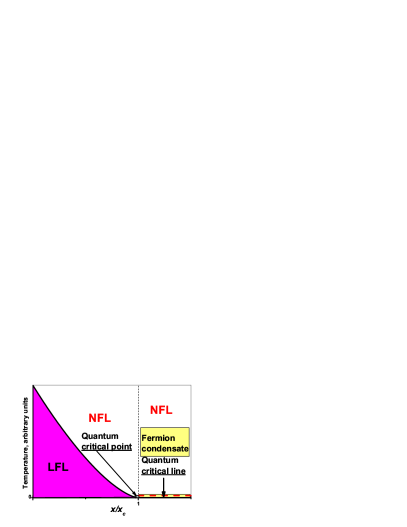
Figure 1: Schematic phase diagram of the system driven to the FC state. The number density $x$ is taken as the control parameter and depicted as $x/x_{c}$. The quantum critical point (QCP), $x/x_{c}=1$, of FCQPT is shown by the arrow. At $x/x_{c}<1$ and sufficiently low temperatures, the system is in the Landau Fermi liquid (LFL) state as shown by the shadow area. At $T=0$ and beyond QCP, $x/x_{c}>1$, the system is at the quantum critical line depicted by the dash line and shown by the vertical arrow. The critical line is characterized by the FC state with finite superconducting order parameter $\kappa$. At $T_{c}=0$, the order parameter $\kappa$ is destroyed, the system undergoes the first order phase transition and exhibits the NFL behavior at $T>0$.

Schematic phase diagram of the system which is driven to FC by variation of $x$ is reported in Fig. 1. Upon approaching the critical density $x_{c}$ the system remains in LFL region at sufficiently low temperatures khodb ; obz , that is shown by the shadow area. At QCP $x_{c}$ shown by the arrow in Fig. 1, the system demonstrates the NFL behavior down to the lowest temperatures. Beyond QCP at finite temperatures the behavior is remaining the NFL one and is determined by the temperature-independent entropy $S_{0}$ yakov . In that case at $T\to 0$, the system is approaching a quantum critical line (shown by the vertical arrow and the dashed line in Fig. 1) rather than a quantum critical point. Upon reaching the quantum critical line from the above at $T\to 0$ the system undergoes the first order quantum phase transition, which is FCQPT taking place at $T_{c}=0$.

At $T>0$ the NFL state above the critical line, see Fig. 1, is strongly degenerated, therefore it is captured by the other states such as superconducting (for example, by the superconducting state in $\rm CeCoIn_{5}$ shag1 ; shag2 ; yakov ) or by AF state (e.g. AF one in $\rm YbRh_{2}Si_{2}$ plaq ) lifting the degeneracy. The application of magnetic field $B>B_{c0}$ restores the LFL behavior, where $B_{c0}$ is a critical magnetic field, such that at $B>B_{c0}$ the system is driven towards its Landau Fermi liquid (LFL) regime shag2 . In some cases, for example in HF metal $\rm CeRu_{2}Si_{2}$, $B_{c0}=0$, see e.g. takah , while in $\rm YbRh_{2}Si_{2}$, $B_{c0}\simeq 0.06$ T geg . In our simple model $B_{c0}$ is taken as a parameter.

Schematic phase diagram of the HF metal $\rm YbRh_{2}Si_{2}$ is reported in Fig. 2. Magnetic field $B$ is taken as the control parameter. The FC state and the region lying at $x/x_{c}\geq 1$, see Fig. 1, can be captured by the superconducting, ferromagnetic, antiferromagnetic (AF) etc. states lifting the degeneracy obz ; khodb . Since we consider the HF metal $\rm YbRh_{2}Si_{2}$ the AF state takes place geg as shown in Fig. 2. As seen from Fig. 2, at elevated temperatures and fixed magnetic field the NFL regime occurs, while rising $B$ again drives the system from NFL region to LFL one. Below we consider the transition region when at rising $B$ the system moves from NFL regime to LFL one along the dash-dot horizontal arrow, and at elevated $T$ it moves from LFL regime to NFL one along the solid vertical arrow.

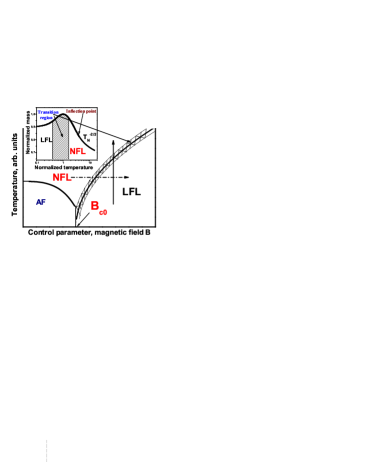
Figure 2: Schematic phase diagram of the HF metal $\rm YbRh_{2}Si_{2}$. $B_{c0}$ is magnetic field at which the effective mass diverges. $\rm{AF}$ denotes antiferromagnetic (AF) state. At $B<B_{c0}$ the system is in AF state. The vertical arrow shows the transition from the LFL regime to the NFL one at fixed $B$ along $T$ with $M^{*}$ depending on $T$. The dash-dot horizontal arrow illustrates the system moving from NFL regime to LFL one along $B$ at fixed $T$. The inset shows a schematic plot of the scaling behavior of the normalized effective mass versus the normalized temperature. Transition regime, where $M^{*}_{N}$ reaches its maximum value $M^{*}_{M}$ at $T=T_{M}$, is shown by the hatched area both in the main panel and in the inset. The arrows mark the position of inflection point in $M^{*}_{N}$ and the transition region.

To explore a scaling behavior of $M^{*}$, we write the quasiparticle distribution function as $n_{1}({\bf p})=n({\bf p},T)-n({\bf p})$, with $n({\bf p})$ is the step function, and Eq. (3) then becomes

$$\frac{1}{M^{*}(T)}=\frac{1}{M^{*}}+\int\frac{{\bf p}_{F}{\bf p_{1}}}{p_{F}^{3}}F({\bf p_{F}},{\bf p}_{1})\frac{\partial n_{1}(p_{1},T)}{\partial p_{1}}\frac{d{\bf p}_{1}}{(2\pi)^{3}}.$$ (5)

At QCP the effective mass $M^{*}$ diverges and Eq. (5) becomes homogeneous determining $M^{*}$ as a function of temperature

$$M^{*}(T)\propto T^{-2/3},$$ (6)

while the system exhibits the NFL behavior ckz ; obz . If the system is located before QCP, $M^{*}$ is finite, at low temperatures the system demonstrates the LFL behavior that is $M^{*}(T)\simeq M^{*}+a_{1}T^{2}$, with $a_{1}$ is a constant, see the inset to Fig. 2. Obviously, the LFL behavior takes place when the second term on the right hand side of Eq. (5) is small in comparison with the first one. Then, at rising temperatures the system enters the transition regime: $M^{*}$ grows, reaching its maximum $M^{*}_{M}$ at $T=T_{M}$, with subsequent diminishing. Near temperatures $T\geq T_{M}$ the last ”traces” of LFL regime disappear, the second term starts to dominate, and again Eq. (5) becomes homogeneous, and the NFL behavior restores, manifesting itself in decreasing $M^{*}$ as $T^{-2/3}$. When the system is near QCP, it turns out that the solution of Eq. (5) $M^{*}(T)$ can be well approximated by a simple universal interpolating function obz ; ckz ; shag2 . The interpolation occurs between the LFL ($M^{*}\simeq M^{*}+a_{1}T^{2}$) and NFL ($M^{*}\propto T^{-2/3}$) regimes thus describing the above crossover ckz ; obz . Introducing the dimensionless variable $y=T_{N}=T/T_{M}$, we obtain the desired expression

$$M^{*}_{N}(y)\approx c_{0}\frac{1+c_{1}y^{2}}{1+c_{2}y^{8/3}}.$$ (7)

Here $M^{*}_{N}=M^{*}/M^{*}_{M}$ is the normalized effective mass, $c_{0}=(1+c_{2})/(1+c_{1})$, $c_{1}$ and $c_{2}$ are fitting parameters, parameterizing the Landau amplitude.

The inset to Fig. 2 demonstrates the scaling behavior of the normalized effective mass $M^{*}_{N}=M^{*}/M^{*}_{M}$ versus normalized temperature $T_{N}=T/T_{M}$, where $M^{*}_{M}$ is the maximum value that $M^{*}$ reaches at $T=T_{M}$. At $T\ll T_{M}$ the LFL regime takes place. At $T\gg T_{M}$ the $T^{-2/3}$ regime takes place. This is marked as NFL one since the effective mass depends strongly on temperature. The temperature region $T\simeq T_{M}$ signifies the transition between the LFL regime with almost constant effective mass and NFL behavior, given by $T^{-2/3}$ dependence. Thus temperatures $T\sim T_{M}$ can be regarded as the transition region between LFL and NFL regimes. The transition temperatures are not really a phase transition. These necessarily are broad, very much depending on the criteria for determination of the point of such a transition, as it is seen from the inset to Fig. 2. As usually, the transition temperature is extracted from the temperature dependence of charge transport, for example, from the resistivity $\rho(T)=\rho_{0}+AT^{2}$ with $\rho_{0}$ is the residual resistivity and $A$ is the LFL coefficient. The crossover takes place at temperatures where the resistance starts to deviate from the LFL $T^{2}$ behavior. Obviously, the measure of the deviation from the LFL $T^{2}$ behavior cannot be defined unambiguously. Therefore, different measures produce different results.

It is possible to transport Eq. (5) to the case of the application of magnetic fields ckz ; obz ; shag2 . The application of magnetic field restores the LFL behavior so that $M^{*}_{M}$ depends on $B$ as

$$M^{*}_{M}\propto(B-B_{c0})^{-2/3},$$ (8)

while

$$T_{M}\propto\mu_{B}(B-B_{c0}),$$ (9)

where $\mu_{B}$ is the Bohr magneton ckz ; shag2 ; obz . Employing Eqs. (8) and (9) to calculate $M^{*}_{M}$ and $T_{M}$, we conclude that Eq. (7) is valid to describe the normalized effective mass in external fixed magnetic fields with $y=T/(B-B_{c0})$. On the other hand, Eq. (7) is valid when the applied magnetic field becomes a variable, while temperature is fixed $T=T_{f}$. In that case, as seen from Eqs. (6), (7) and(8), it is convenient to rewrite both the variable as $y=(B-B_{c0})/T_{f}$, and Eq. (9) as

$$\mu_{B}(B_{M}-B_{c0})\propto T_{f}.$$ (10)

It follows from Eq. (7) that in contrast to the Landau paradigm of quasiparticles the effective mass strongly depends on $T$ and $B$. As we will see it is this dependence that forms the NFL behavior. It follows also from Eq. (7) that a scaling behavior of $M^{*}$ near QCP is determined by the absence of appropriate external physical scales to measure the effective mass and temperature. At fixed magnetic fields, the characteristic scales of temperature and of the function $M^{*}(T,B)$ are defined by both $T_{M}$ and $M^{*}_{M}$ respectively. At fixed temperatures, the characteristic scales are $(B_{M}-B_{c0})$ and $M^{*}_{M}$. It follows from Eqs. (8) and (9) that at fixed magnetic fields, $T_{M}\to 0$, and $M^{*}_{M}\to\infty$, and the width of the transition region shrinks to zero as $B\to B_{c0}$ when these are measured in the external scales. In the same way, it follows from Eqs. (6) and (10) that at fixed temperatures, $(B_{M}-B_{c0})\to 0$, and $M^{*}_{M}\to\infty$, and the width of the transition region shrinks to zero as $T_{f}\to 0$. Thus, the application of the external scales obscure the scaling behavior of the effective mass and thermodynamic and transport properties.

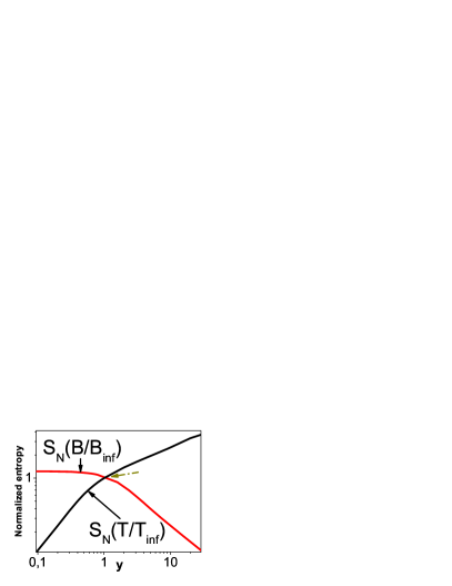
Figure 3: The normalized entropy $S_{N}(B/B_{inf})$ versus $y=B/B_{inf}$ and the normalized entropy $S_{N}(T/T_{inf})$ versus $y=T/T_{inf}$ calculated at fixed temperature and magnetic field, correspondingly, are represented by the solid lines and shown by the arrows. The inflection point is depicted by the dash-dot arrow.

A few remarks are in order here. As we shall see, magnetic field dependencies of the effective mass or of other observable like the longitudinal magnetoresistance do not have ”peculiar points” like maximum. The normalization are to be performed in the other points like the inflection point at $T=T_{inf}$ (or at $B=B_{inf}$) shown in the inset to Fig. 2 by the arrow. Such a normalization is possible since it is established on the internal scales, $T_{inf}\propto T_{M}\propto(B-B_{c0})$.

In what follows, we compute the effective mass and employ Eq. (7) for estimations of considered values. To compute the effective mass $M^{*}(T,B)$, we solve Eq. (5) with special form of Landau interaction amplitude, see Refs. ckz ; obz for details. Choice of the amplitude is dictated by the fact that the system has to be at QCP, which means that first two $p$-derivatives of the single-particle spectrum $\varepsilon({\bf p})$ should equal zero. Since first derivative is proportional to the reciprocal quasiparticle effective mass $1/M^{*}$, its zero just signifies QCP of FCQPT. Zeros of two subsequent derivatives mean that the spectrum $\varepsilon({\bf p})$ has an inflection point at $p_{F}$ so that the lowest term of its Taylor expansion is proportional to $(p-p_{F})^{3}$ ckz . After solution of Eq. (5), the obtained spectrum had been used to calculate the entropy $S(B,T)$, which, in turn, had been recalculated to the effective mass $M^{*}(T,B)$ by virtue of well-known LFL relation $M^{*}(T,B)=S(T,B)/T$. Our calculations of the normalized entropy as a function of the normalized magnetic field $B/B_{inf}=y$ and as a function of the normalized temperature $y=T/T_{inf}$ are reported in Fig. 3. Here $T_{inf}$ and $B_{inf}$ are the corresponding inflection points in function $S$. We normalize the entropy by its value at the inflection point $S_{N}(y)=S(y)/S(1)$. As seen form Fig. 3, our calculations corroborate the scaling behavior of the normalized entropy, that is the curves at different temperatures and magnetic fields merge into single one in terms of the variable $y$. The inflection point $T_{inf}$ in $S(T)$ makes $M^{*}(T,B)$ have its maximum as a function of $T$, while $M^{*}(T,B)$ versus $B$ has no maximum. We note that our calculations of the entropy confirm the validity of Eq. (7) and the scaling behavior of the normalized effective mass.

Exciting measurements of $C/T\propto M^{*}$ on samples of the new generation of $\rm YbRh_{2}Si_{2}$ in different magnetic fields $B$ up to 1.5 T oes allow us to identify the scaling behavior of the effective mass $M^{*}$ and observe the different regimes of $M^{*}$ behavior such as the LFL regime, transition region from LFL to NFL regimes, and the NFL regime itself. A maximum structure in $C/T\propto M^{*}_{M}$ at $T_{M}$ appears under the application of magnetic field $B$ and $T_{M}$ shifts to higher $T$ as $B$ is increased. The value of $C/T=\gamma_{0}$ is saturated towards lower temperatures decreasing at elevated magnetic field, where $\gamma_{0}$ is the Sommerfeld coefficient oes .

The transition region corresponds to the temperatures where the vertical arrow in the main panel of Fig. 2 crosses the hatched area. The width of the region, being proportional to $T_{M}\propto(B-B_{c0})$ shrinks, $T_{M}$ moves to zero temperature and $\gamma_{0}\propto M^{*}$ increases as $B\to B_{c0}$. These observations are in accord with the facts oes .

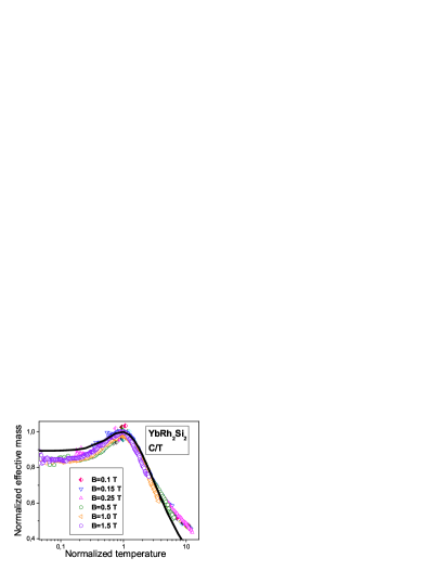
Figure 4: The normalized effective mass $M^{*}_{N}$ extracted from the measurements of the specific heat $C/T$ on $\rm YbRh_{2}Si_{2}$ in magnetic fields $B$ oes listed in the legend. Our calculations are depicted by the solid curve tracing the scaling behavior of $M^{*}_{N}$.

To obtain the normalized effective mass $M^{*}_{N}$, the maximum structure in $C/T$ was used to normalize $C/T$, and $T$ was normalized by $T_{M}$. In Fig. 4 $M^{*}_{N}$ as a function of normalized temperature $T_{N}$ is shown by geometrical figures, our calculations are shown by the solid line. Figure 4 reveals the scaling behavior of the normalized experimental curves - the scaled curves at different magnetic fields $B$ merge into a single one in terms of the normalized variable $y=T/T_{M}$. As seen, the normalized mass $M^{*}_{N}$ extracted from the measurements is not a constant, as would be for LFL. The two regimes (the LFL regime and NFL one) separated by the transition region, as depicted by the hatched area in the inset to Fig. 2, are clearly seen in Fig. 4 illuminating good agreement between the theory and facts. It is worthy of note that the normalization procedure allows us to construct the scaled function $C/T$ extracted from the facts in wide range variation of the normalized temperature. Indeed, it integrates measurements of $C/T$ taken at the application of different magnetic fields into unique function which demonstrates the scaling behavior over three decades in normalized temperature as seen from Fig. 4.

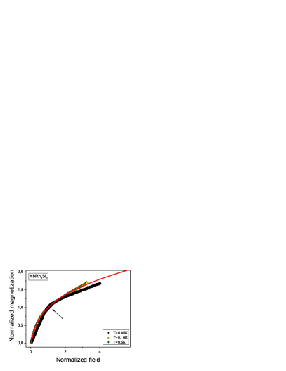
Figure 5: The field dependencies of the normalized magnetization $M$ collected at different temperatures shown at right bottom corner are extracted from measurements collected on $\rm{YbRu_{2}Si_{2}}$ steg . The kink (shown by the arrow) is clearly seen at the normalized field $B_{N}=B/B_{k}\simeq 1$. The solid curve represents our calculations.

Consider now the magnetization $M$ as a function of magnetic field $B$ at fixed temperature $T=T_{f}$

$$M(B,T)=\int_{0}^{B}\chi(b,T)db,$$ (11)

where the magnetic susceptibility $\chi$ is given by land

$$\chi(B,T)=\frac{\beta M^{*}(B,T)}{1+F_{0}^{a}}.$$ (12)

Here, $\beta$ is a constant and $F_{0}^{a}$ is the Landau amplitude related to the exchange interaction land . In the case of strongly correlated systems $F_{0}^{a}\geq-0.9$ pfit ; pfit1 . Therefore, as seen from Eq. (12), due to the normalization the coefficients $\beta$ and $(1+F_{0}^{a})$ drops out from the result, and $\chi\propto M^{*}$.

One might suppose that $F_{0}^{a}$ can strongly depend on $B$. This is not the case, since the Kadowaki-Woods ratio is conserved kadw ; geg1 ; kwz , $A(B)/\gamma_{0}^{2}(B)\propto A(B)/\chi^{2}(B)\propto const$, we have $\gamma_{0}\propto M^{*}\propto\chi$. Here $A$ is the coefficient in the $T^{2}$ dependence of resistivity $\rho$.

Our calculations show that the magnetization exhibits a kink at some magnetic field $B=B_{k}$. The experimental magnetization demonstrates the same behavior steg . We use $B_{k}$ and $M(B_{k})$ to normalize $B$ and $M$ respectively. The normalized magnetization $M(B)/M(B_{k})$ extracted from facts steg depicted by the geometrical figures and calculated magnetization shown by the solid line are reported in Fig. 5. As seen, the scaled data at different $T_{f}$ merge into a single one in terms of the normalized variable $y=B/T_{k}$. It is also seen, that these exhibit energy scales separated by kink at the normalized magnetic field $B_{N}=B/B_{k}=1$. The kink is a crossover point from the fast to slow growth of $M$ at rising magnetic field. It is seen from Fig. 5, that our calculations are in good agreement with the facts, and all the data exhibit the kink (shown by the arrow) at $B_{N}\simeq 1$ taking place as soon as the system enters the transition region corresponding to the magnetic fields where the horizontal dash-dot arrow in the main panel of Fig. 2 crosses the hatched area. Indeed, as seen from Fig. 5, at lower magnetic fields $M$ is a linear function of $B$ since $M^{*}$ is approximately independent of $B$. Then, it follows from Eqs. (7) and (8) that at elevated magnetic fields $M^{*}$ becomes a diminishing function of $B$ and generates the kink in $M(B)$ separating the energy scales discovered in Refs. steg1 ; steg . Then, as seen from Eq. (10) the magnetic field $B_{k}$ at which the kink appears, $B_{k}\simeq B_{M}\propto T_{f}$, shifts to lower $B$ as $T_{f}$ is decreased. This observation is in accord with facts steg1 ; steg .

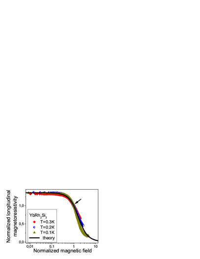
Figure 6: Magnetic field dependence of the normalized magnetoresistance $\rho_{N}$ versus normalized magnetic field. $\rho_{N}$ was extracted from LMR of $\rm YbRh_{2}Si_{2}$ at different temperatures steg1 ; steg listed in the legend. The inflection point is shown by the arrow, and the solid line represents our calculations.

Consider a longitudinal magnetoresistance (LMR) $\rho(B,T)=\rho_{0}+AT^{2}$ as a function of $B$ at fixed $T_{f}$. In that case, the classical contribution to LMR due to orbital motion of carriers induced by the Lorentz force is small, while the Kadowaki-Woods relation kadw ; geg1 ; kwz , $K=A/\gamma_{0}^{2}\propto A/\chi^{2}=const$, allows us to employ $M^{*}$ to construct the coefficient $A$ pla3 , since $\gamma_{0}\propto\chi\propto M^{*}$. As a result, $\rho(B,T)-\rho_{0}\propto(M^{*})^{2}$. Fig. 6 reports the normalized magnetoresistance

$$\rho_{N}(y)=\frac{\rho(y)-\rho_{0}}{\rho_{inf}}\propto(M_{N}^{*}(y))^{2}$$ (13)

versus normalized magnetic field $y=B/B_{inf}$ at different temperatures, shown in the legend. Here $\rho_{inf}$ and $B_{inf}$ are LMR and magnetic field respectively taken at the inflection point marked by the arrow in Fig. 6. Both theoretical (shown by the solid line) and experimental (marked by the geometrical figures) curves have been normalized by their inflection points, which also reveals the scaling behavior - the scaled curves at different temperatures merge into single one as a function of the variable $y$ and show the scaling behavior over three decades in the normalized magnetic field. The transition region at which LMR starts to decrease is shown in the inset to Fig. 2 by the hatched area. Obviously, as seen from Eq. (10), the width of the transition region being proportional to $B_{M}\simeq B_{inf}\propto T_{f}$ decreases as the temperature $T_{f}$ is lowered. In the same way, the inflection point of LMR, generated by the inflection point of $M^{*}$ shown in the inset to Fig. 2 by the arrow, shifts to lower $B$ as $T_{f}$ is decreased. All these observations are in excellent agreement with the facts steg1 ; steg .

The evolution of the derivative of magnetic entropy $dS(B,T)/dB$ as a function of magnetic field $B$ at fixed temperature $T_{f}$ is of great importance since it allows us to study the scaling behavior of the derivative of the effective mass $TdM^{*}(B,T)/dB\propto dS(B,T)/dB$. While the scaling properties of the effective mass $M^{*}(B,T)$ can be analyzed via LMR, see Fig. 6.

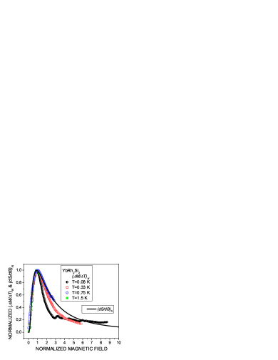
Figure 7: Normalized magnetization difference divided by temperature increment $(\Delta M/\Delta T)_{N}$ versus normalized magnetic field at fixed temperatures listed in the legend is extracted from the facts collected on $\rm YbRh_{2}Si_{2}$ geg . Our calculation of the normalized derivative $(dS/dB)_{N}\simeq(\Delta M/\Delta T)_{N}$ versus normalized magnetic field is shown by the solid line.

As seen from from Eqs. (7) and (10), at $y\leq 1$ the derivative $-dM_{N}(y)/dy\propto y$ with $y=(B-B_{c0})/(B_{inf}-B_{c0})\propto(B-B_{c0})/T_{f}$. We note that the effective mass as a function of $B$ does not have the maximum. At elevated $y$ the derivative $-dM_{N}(y)/dy$ possesses a maximum at the inflection point and then becomes a diminishing function of $y$. Upon using the variable $y=(B-B_{c0})/T_{f}$, we conclude that at decreasing temperatures, the leading edge of the function $-dS/dB\propto-TdM^{*}/dB$ becomes steeper and its maximum at $(B_{inf}-B_{c0})\propto T_{f}$ is higher. These observations are in quantitative agreement with striking measurements of the magnetization difference divided by temperature increment, $-\Delta M/\Delta T$, as a function of magnetic field at fixed temperatures $T_{f}$ collected on $\rm YbRh_{2}Si_{2}$ geg . We note that according to the well-know thermodynamic equality $dM/dT=dS/dB$, and $\Delta M/\Delta T\simeq dS/dB$. To carry out a quantitative analysis of the scaling behavior of $-dM^{*}(B,T)/dB$, we calculate the normalized entropy $S$ shown in Fig. 3 as a function of $B/B_{inf}$ at fixed temperature $T_{f}$. Fig. 7 reports the normalized $(dS/dB)_{N}$ as a function of the normalized magnetic field. The scaled function $(dS/dB)_{N}$ is obtained by normalizing $(-dS/dB)$ by its maximum taking place at $B_{M}$, and the field $B$ is scaled by $B_{M}$. The measurements of $-\Delta M/\Delta T$ are normalized in the same way and depicted in Fig. 7 as $(\Delta M/\Delta T)_{N}$ versus normalized field. It is seen from Fig. 7 that our calculations shown by the solid line are in good agreement with the facts and the scaled functions $(\Delta M/\Delta T)_{N}$ extracted from the facts show the scaling behavior in wide range variation of the normalized magnetic field $B/B_{M}$.

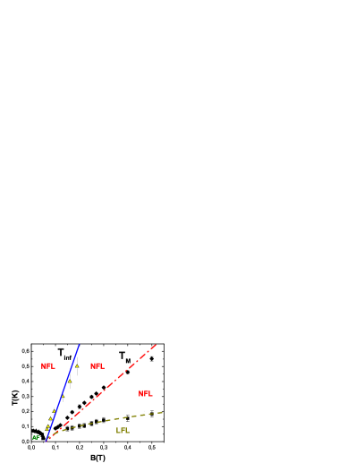
Figure 8: Temperature versus magnetic field $T-B$ phase diagram for $\rm YbRh_{2}Si_{2}$. Solid circles represent the boundary between AF and NFL states. The solid squares denote the boundary of the NFL and LFL regime steg1 ; steg ; geg1 shown by the dotted line which is approximated by $\sqrt{B-B_{c0}}$ obz . Diamonds mark the maximums $T_{M}$ of $C/T$ oes shown in Fig. 4. The dash-dot line is approximated by $T_{M}\propto a(B-B_{c0})$, $a$ is a fitting parameter, see Eq. (9). Triangles along the solid line denote $T_{inf}$ in LMR steg1 ; steg sown in Fig. 7, the solid line represents the function $T_{inf}\propto b(B-B_{c0})$, $b$ is a fitting parameter, see Eq. (10).

Fig. 8 reports $T_{inf}$ and $T_{M}$ versus $B$ depicted by the solid and dash-dotted lines, respectively. The boundary between the NFL and LFL regimes is shown by the dashed line, and AF marks the antiferromagnetic state. The corresponding data are taken from Ref. steg1 ; steg ; oes ; geg1 . It is seen that our calculations are in good agreement with the facts. In Fig. 8, the solid and dash-dotted lines corresponding to the functions $T_{inf}$ and $T_{M}$, respectively, represent the positions of the kinks separating the energy scales in $C$ and $M$ reported in Ref. steg1 ; steg . It is seen that our calculations are in accord with facts, and we conclude that the energy scales are reproduced by Eqs. (9) and (10) and related to the peculiar points $T_{inf}$ and $T_{M}$ of the normalized effective mass $M^{*}_{N}$ which are shown by the arrows in the inset to Fig. 2.

At $B\to B_{c0}$ both $T_{inf}\to 0$ and $T_{M}\to 0$, thus the LFL and the transition regimes of both $C/T$ and $M$ as well as these of LMR and the magnetic entropy are shifted to very low temperatures. Therefore due to experimental difficulties these regimes cannot be often observed in experiments on HF metals. As it is seen from Figs. 4, 5, 6, 7 and 8, the normalization allows us to construct the unique scaled thermodynamic and transport functions extracted from the experimental facts in wide range of the variation of the scaled variable $y$. As seen from the mentioned Figures, the constructed normalized thermodynamic and transport functions show the scaling behavior over three decades in the normalized variable.

In summary, we have analyzed the non-Fermi liquid behavior of the heavy fermion metals, and showed that extended quasiparticles paradigm is strongly valid, while the dependence of the effective mass on temperature, number density and applied magnetic fields gives rise to the NFL behavior. We have demonstrated that our theoretical study of the heat capacity, magnetization, longitudinal magnetoresistance and magnetic entropy are in good agreement with the outstanding recent facts collected on the HF metal $\rm YbRh_{2}Si_{2}$. Our normalization procedure has allowed us to construct the scaled thermodynamic and transport properties in wide range of the variation of the scaled variable. For $\rm YbRh_{2}Si_{2}$ the constructed thermodynamic and transport functions show the scaling behavior over three decades in the normalized variable. The energy scales in these functions are also explained.

This work was supported in part by the grants: RFBR No. 09-02-00056 and the Hebrew University Intramural Funds. V.R.S. is grateful to the Lady Davis Foundation for supporting his visit to the Hebrew University of Jerusalem.

References

- (1) T. Senthil, M. Vojta, and S. Sachdev, Phys. Rev. B 69, 035111 (2004).
- (2) P. Coleman and A.J. Schofield, Nature 433, 226 (2005).
- (3) H.v. Löhneysen, A. Rosch, M. Vojta, and P. Wölfle, Rev. Mod. Phys. 79, 1015 (2007).
- (4) P. Gegenwart, Q. Si, and F. Steglich, Nature Phys. 4, 186 (2008).
- (5) S. Sachdev, Nature Phys. 4, 173 (2008).
- (6) P. Coleman et al., J. Phys. Condens. Matter 13, R723 (2001).
- (7) V.A. Khodel, JETP Lett. 86, 721 (2007); V.A. Khodel, J.W. Clark, and M.V. Zverev, arXiv: 0904.1509
- (8) E.M. Lifshitz and L.P. Pitaevskii, Statistical Physics, Part 2, Butterworth-Heinemann, Oxford, 1999.
- (9) V.A. Khodel and V.R. Shaginyan, JETP Lett. 51, 553 (1990).
- (10) M. Ya. Amusia and V.R. Shaginyan, Phys. Rev. B63, 224507 (2001).
- (11) G.E. Volovik, Springer Lecture Notes in Physics 718, 31 (2007).
- (12) V.R. Shaginyan, M.Ya. Amusia, and K.G. Popov, Physics-Uspekhi 50, 563 (2007).
- (13) V.A. Khodel, J.W. Clark, and M.V. Zverev, Phys. Rev. B78, 075120 (2008).
- (14) J. Dukelsky et. al., Z. Phys. B: Condens. Matter 102, 245 (1997).
- (15) J.W. Clark, V.A. Khodel, and M.V. Zverev Phys. Rev. B71, 012401 (2005).
- (16) V.R. Shaginyan, M.Ya. Amusia, and K.G. Popov, Phys. Lett. A 373, 2281 (2009).
- (17) P. Gegenwart et. al., Science 315, 969 (2007).
- (18) N. Oeschler et. al., Physica B 403, 1254 (2008).
- (19) P. Gegenwart et. al., Physica B 403, 1184 (2008).
- (20) Y. Tokiwa et. al., Phys. Rev. Lett. 102, 066401 (2009).
- (21) V.R. Shaginyan et. al., Europhys. Lett. 76, 898 (2006).
- (22) V.R. Shaginyan, K.G. Popov, and V.A. Stephanovich, Europhys. Lett. 79, 47001 (2007).
- (23) L.N. Oliveira, E.K.U. Gross, and W. Kohn, Phys. Rev. Lett. 60, 2430 (1988).
- (24) V.A. Khodel, M.V. Zverev, and V.M. Yakovenko, Phys. Rev. Lett. 95, 236402 (2005).
- (25) V.R. Shaginyan, Phys. Lett. A 249, 237 (1998).
- (26) M. Pfitzner and P. Wölfle, Phys. Rev. B 33, 2003 (1986).
- (27) D. Wollhardt, P. Wölfle, and P.W. Anderson, Phys. Rev. B35, 6703 (1987).
- (28) V.R. Shaginyan, A. Z. Msezane, K. G. Popov, and V. A. Stephanovich, Phys. Rev. Lett. 100, 096406 (2008).
- (29) D. Takahashi et al., Phys. Rev. B 67, 180407(R) (2003).
- (30) K. Kadowaki and S.B. Woods, Solid State Commun. 58, 507 (1986).
- (31) P. Gegenwart et al., Phys. Rev. Lett. 89, 056402 (2002).
- (32) A. Khodel and P. Schuck, Z. Phys. B: Condens. Matter 104, 505 (1997).
- (33) V.R. Shaginyan et al., Phys. Lett. A 373, 986 (2009).