Effective density of states for a quantum oscillator coupled to a photon field

Abstract. We give an explicit formula for the effective partition function of a harmonically bound particle minimally coupled to a photon field in the dipole approximation. The effective partition function is shown to be the Laplace transform of a positive Borel measure, the effective measure of states. The absolutely continuous part of the latter allows for an analytic continuation, the singularities of which give rise to resonances. We give the precise location of these singularities, and show that they are well approximated by of first order poles with residues equal the multiplicities of the corresponding eigenspaces of the uncoupled quantum oscillator. Thus we obtain a complete analytic description of the natural line spectrum of the charged oscillator.

Keywords: Resonances, Pauli-Fierz model, density of states, partition function, line broadening

2010 Math. Subj. Class.: 81V10, 82B10

1. Introduction

The standard model for a non-relativistic quantum particle interacting with the radiation field is the Pauli-Fierz model using minimal coupling. The Hamiltonian is

$$H=\frac{1}{2m}(p-eA)^{2}+V+H_{\rm f},$$ (1.1)

where $H_{\rm f}$ is the Hamiltonian of the free field, $A$ is the transverse quantized field and $e$ the electron charge, $p$ is the particle momentum and $V$ the particle potential. We do not introduce form factors. Over the last years, there has been much activity and significant progress in understanding the Pauli-Fierz model. Notable developments include the proof of existence for a ground state when the infrared cutoff is removed [9], a detailed spectral analysis of the Hamiltonian and the proof of the existence of resonaces [1], and a proof of enhanced binding through the photon field [10]. We refrain from giving a review of the by now vast literature on the subject, and instead refer to [18] and the bibliography therein.

As is apparent already from the above selection of results, the majority of works on the subject investigates the spectral structure of the full system, particle and field. In our work, instead we regard the photon field as an environment in which the particle is embedded. A prominent example of this point of view is Feynman’s polaron [8] by which our present investigations are inspired. The aim is to treat the coupled particle as a closed system, and to derive, for the particle alone, effective equations that capture the influence of the photon field. The particular effective quantity that we investigate (and, to our knowledge, indeed introduce) is the effective measure of states.

We consider a version of (1.1) that is simplified in two ways: Firstly, we use the dipole approximation, which amounts to replacing $A$ with $A(0)$, and secondly we omit the self-interaction $A^{2}$ of the field. (The omission of the $A^{2}$ term is necessary only for a part of our calculations, and we discuss the possibility of keeping it in the final remark of Section 3.) The particle potential $V$ is taken to be harmonic, so that $H$ is completely quadratic, and we add the well-known terms of mass and energy renormalization. In this setup we compute the ratio $Z$ of the partition functions of the full system and of the free field. We do this by first suitably discretizing both systems, and then taking the continuous-mode limit and the ultraviolet limit. This procedure yields a finite result. We find the explicit expression

$$Z(\beta)=\left[\frac{\rho}{2\pi}\emph{e}^{-2\rho\ln(\rho)\sin\varphi}\left|\Gamma({\rm i}\rho\,\emph{e}^{-{\rm i}\varphi})\right|^{2}\right]^{3}$$ (1.2)

with $\rho\,\sim\beta$ inversely proportional to the temperature $T$ and sin$\varphi\sim e^{2}$ determining the strength of the coupling. See Theorem 3.3 for details.

From the ratio $Z$ of the partition functions one gets an explicit expression for the difference of the respective free energies. Subtracting from this the free energy $F_{0}$ of the particle leads to the excess free energy $F_{\rm ex}=-(\hbar/\beta)\ln(Z/Z_{0})$. The latter is particularly interesting in that it is supposed to be experimentally accessible. Referring to [4] we only mention that (1.2) confirms the well-known quadratic low-temperature behavior

$$F_{\rm ex}(\beta)\approx-\pi\alpha{\rm k}^{2}T^{2}(3mc^{2})^{-1}$$ (1.3)

of the excess free energy.

In the present case, however, the significance of $Z$ goes beyond that. As we will argue in Section 2.3 for general coupled systems, (1.2) is the effective partition function (or partition function for the particle subsystem). This means that $Z$ replaces $Z_{0}$ when the small system is regarded as autonomous while retaining an effective influence of the field. The central fact is that, as we prove, $Z$ is the Laplace transform of a positive Borel measure $\mu$. We interpret $\mu$ as the effective measure of states for the charged oscillator. It has the same significance for the effective system that the measure of states $\mu_{0}$ (whose Laplace transform is $Z_{0}$, see (2.1) and (2.2)), has for the uncoupled oscillator. It determines the probabilities of energy measurements at the system in thermal equilibrium.

It is worth remembering that in general the ratio of two partition functions is not the Laplace transform of some positive Borel measure. Most probably this is the case here as long as in the derivation of (1.2) the ultraviolet cutoff $C$ is kept finite (even if the continuous-mode limit is already done). But a finite cutoff in not desirable in any case, as any result we obtain for the effective system would depend on the arbitrary parameter $C$. Thus it is crucial that the ultraviolet limit can be carried out, leading to an expression that is the Laplace transform of a positive measure.

Formula (1.2) allows a detailed study of the effective measure of states. First of all, it turns out that $\mu$ has one atom at the ground state frequency $\omega_{\varphi}$, is supported on the half line $[\omega_{\varphi},\infty[$, and is otherwise absolutely continuous with respect to Lebesgue measure. The corresponding density $\phi$ will be called effective density of states. We prove that $\phi$ has an analytic continuation with singularities and cuts along the boundary of a cone with apex $\omega_{\varphi}$ and opening angle $2\varphi$. The conjugate pairs of singularities can be approximated by first order singularities in the interior of the cone, up to logarithmic corrections. The position and residue of these first order poles can be determined analytically. On the real line, they give rise to Lorentz profiles that replace the Dirac peaks present in $\mu_{0}$. The mass of each Lorentz profile is equal to the mass of the corresponding Dirac peak, and its position agrees with predictions of QED time-dependent perturbation theory up to first order in the fine structure constant $\alpha$. See Theorems 3.5 and 3.6 and the remarks following them for details.

From the above properties, a connection of the effective density of states with the theory of resonances appears obvious. The latter occur when a small quantum system is coupled to a quantum field or reservoir, at which point eigenvalues of the small system dissolve into the continuous spectrum, and stationary states change into metastable states. In the Pauli-Fierz model, resonances have been investigated extensively by Bach, Fröhlich and Sigal in [1]. These authors employ the well-established complex dilation method. They study the spectrum of the full system, particle and field; resonances are then defined as the singularities of the analytic continuation of the resolvent to the second Riemann sheet. In contrast, we work in the context of open quantum systems, and therefore the effective small system does not even have a Hamiltonian. While there has been work on resonances and decoherence in open quantum systems, such as [2] and [14, 15], all authors seem to rely on the spectral structure of the full Hamiltonian.

We define a resonance of an effective system in Definition 3, in terms of the complex structure of the effective density of states. For the harmonically bound charged particle, we show that this definition, and the concept of the effective density of states in general, produce physically reasonable results. Apart from facilitating explicit formulae, we do not expect the harmonic particle potential to be a vital part of the above picture; we thus conjecture that also for other confined charged systems, the effective density of states exists, and that its complex structure yields an appropriate description of the spectral lines by Lorentz profiles. A proof of this conjecture may well turn out to be challenging, and will probably require some insight into the connections of our results with the theory of [1].

Our paper is organized as follows. In Section 3, we present our model in detail and state the main rigorous results of this work, along with a short discussion. Proofs are given in Sections 4 and 5. The following Section 2 interprets our results in the framework of quantum statistical mechanics, and discusses their connection to the theory of resonances.

Acknowledgments: We would like to thank Herbert Spohn for many useful discussions, and Marco Merkli for helpful comments. V.B. is supported by the EPSRC fellowship EP/D07181X/1.

2. Partition function of the embedded system

We regard the particle as embedded into the environment of the radiation field. An environment is characterized by the fact that it stays in thermal equilibrium if the joint system is in thermal equilibrium. Roughly speaking, the interaction has effects on the embedded system but does not change the environment. More precisely, when acting on the embedded system the environment carries out transitions between same states.

A well-known example of a quantum system whose embedding in the environment determines decisively its properties is the polaron, i.e. an electron in an ionic crystal. The computations in [8, Chapter 8] confirm that the electron moving with its accompanying distortion of the lattice behaves as a free particle but with an effective mass higher than that of the electron. In the same spirit we are going to treat the problem of a charged oscillator surrounded by its own radiation field. In this section we put $\hbar=\rm k=1$.

2.1. Energy distribution in thermal equilibrium

Let the positive operator $H$ be the Hamiltonian of some quantum system. For the moment we assume that $\,{\rm e}^{-\beta H}\,$ is trace class. Classically, the partition function of the system is given by

$$Z(\beta)={\operatorname{Tr\,}}\,{\rm e}^{-\beta H}\,.$$ (2.1)

The inverse Laplace transform $\mu$ of $Z$, which we call the measure of states of the quantum system, is the weighted sum of Dirac measures

$$\mu=\sum_{j}N_{j}\delta_{\lambda_{j}},$$ (2.2)

where $\lambda_{j}$ are the eigenvalues of $H$ and $N_{j}$ are the corresponding finite multiplicities. Its physical relevance is due to the fact that the statistical uncertainty of states of the system in thermal equilibrium at the temperature $T=1/\beta$ is described by the probability measure $\mu^{(\beta)}:=\frac{1}{Z(\beta)}\,{\rm e}^{-\beta(\cdot)}\,\mu$. If $E$ denotes the spectral measure of $H$, and $\Delta$ a Borel subset of ${\mathbb{R}}$, then

$$\mu^{(\beta)}(\Delta)=\frac{1}{Z(\beta)}{\operatorname{Tr\,}}(\,{\rm e}^{-\beta H}\,E(\Delta))$$ (2.3)

is the probability for a measurement of the energy to yield a value in $\Delta$. It is this interpretation that we will retain valid also for the effective entities.

2.2. Spectral discretization

From the basic principle of statistical mechanics, once the partition function is known, all thermodynamic properties can be found. In many interesting cases, however, including our model Hamiltonian (3.1), $\,{\rm e}^{-\beta H}\,$ is not trace class. This raises the problem of how to attribute a partition function to the oscillator embedded in the photon field. The way we solve this problem uses a slight generalization of methods from the theory of random Schrödinger operators (cf. [12]). The main idea is to approximate $H$ by operators $H_{n}$ with discrete spectrum. We define

Definition 1.

Let $H$ be a self-adjoint operator in a Hilbert space ${\mathcal{H}}$, and let $(P_{n})$ be a family of orthogonal projections on ${\mathcal{H}}$. Put $H_{n}=P_{n}HP_{n}$. We say that $H_{n}$ is a spectral discretization of $H$ (associated to $P_{n}$) if

• $P_{n}D(H)\subset D(H)$

• $\lim_{n\to\infty}P_{n}=\rm 1$ in the strong topology.

• The spectrum of $H_{n}$ acting in $P_{n}{\mathcal{H}}$ consists of eigenvalues with finite multiplicity such that $\,{\rm e}^{-\beta H_{n}}\,$ is trace class for all $n$.

2.3. Separation of a subsystem.

Let us now consider a general model consisting of two interacting quantum subsystems with respective state spaces ${\mathcal{H}}_{\rm 1}$ and ${\mathcal{H}}_{\rm 2}$. For convenience, the system corresponding to ${\mathcal{H}}_{1}$ will be called the small system, the other one the large system; but note that there is actually no assumption on the dimension of ${\mathcal{H}}_{1}$ and ${\mathcal{H}}_{2}$. The Hamiltonian of the joint system, acting on ${\mathcal{H}}_{\rm 1}\otimes{\mathcal{H}}_{\rm 2}$ is

$$H=H_{\rm 1}\otimes 1+1\otimes H_{\rm 2}+H_{\rm I},$$ (2.4)

where $H_{\rm I}$ describes the interaction. Again we assume for $H$ the existence of ${\operatorname{Tr\,}}\,{\rm e}^{-\beta H}\,$, and also for $H_{1}$ and $H_{2}$. Let the large system be in thermal equilibrium. Then the influence of it onto the small system can be described in a statistical way by averaging the states of the large system. Accordingly, the density operator attributed to the small system is $W(\beta):=({\operatorname{Tr\,}}\,{\rm e}^{-\beta H_{2}}\,)^{-1}{\operatorname{Tr\,}}_{2}\,{\rm e}^{-\beta H}\,$, where ${\operatorname{Tr\,}}_{2}$ denotes the partial trace with respect to the second factor. In the case $H_{\rm I}=0$ of non-interacting systems, $W(\beta)$ equals $\,{\rm e}^{-\beta H_{1}}\,$. Moreover, if the joint system is in the state $({\operatorname{Tr\,}}\,{\rm e}^{-\beta H}\,)^{-1}\,\,{\rm e}^{-\beta H}\,$, any prediction on measurements which concern only the small system is given by the thus uniquely determined state $({\operatorname{Tr\,}}W(\beta))^{-1}W(\beta)=$ $({\operatorname{Tr\,}}\,{\rm e}^{-\beta H}\,)^{-1}{\operatorname{Tr\,}}_{2}\,{\rm e}^{-\beta H}\,$ of the small system. This is due to the fact that ${\operatorname{Tr\,}}({\operatorname{Tr\,}}_{2}\,{\rm e}^{-\beta H}\,\,E_{1})={\operatorname{Tr\,}}(\,{\rm e}^{-\beta H}\,\;E_{1}\otimes 1)$ holds for every orthogonal projection $E_{1}$ on ${\mathcal{H}}_{1}$ and uniquely determines ${\operatorname{Tr\,}}_{2}$.

Consequently, we regard $Z(\beta):={\operatorname{Tr\,}}W(\beta)$ as the partition function attributed to the small system. It satisfies

$$Z(\beta)=\frac{{\operatorname{Tr\,}}\,{\rm e}^{-\beta H}\,}{{\operatorname{Tr\,}}\,{\rm e}^{-\beta H_{2}}\,},$$ (2.5)

and we will interpret its inverse Laplace transform as the effective measure of states (cf. 2.2) for the small system when in contact with the large system. Of course, for this interpretation to make perfectly sense, $Z$ would need to be the Laplace transform of a positive Borel measure. This is not true in general, but we will find that it does hold in our model when performing the following limiting process.

2.4. Infinitely large environment

The large system in (1.1) is described by $H_{2}=H_{\rm f}$, which has absolutely continuous spectrum on $[0,\infty]$. Thus $\,{\rm e}^{-\beta H_{2}}\,$ is not trace class, and neither is $\,{\rm e}^{-\beta H}\,$, whence (2.5) is not available. We consider spectral discretizations $H_{n}$ and $H_{2,n}$ of $H$ and $H_{2}$, and define

$$Z_{n}(\beta)=\frac{{\operatorname{Tr\,}}\,{\rm e}^{-\beta H_{n}}\,}{{\operatorname{Tr\,}}\,{\rm e}^{-\beta H_{2,n}}\,}.$$ (2.6)

In the case we study $\lim_{n\to\infty}Z_{n}$ exists. After removing an ultraviolet cutoff we get the partition function $Z$, which is the Laplace transform of a positive measure $\mu$ with support in $[0,\infty[$. It is called the effective measure of states of the embedded system. As in Section 2.1 we introduce the probability measures

$$\mu^{(\beta)}=\frac{1}{Z(\beta)}\,{\rm e}^{-\beta(\cdot)}\,\mu$$ (2.7)

for $\beta>0$, which are fundamental in that they determine the probabilities of energy measurements: if the charged oscillator is in thermal equilibrium at the temperature $\frac{1}{\beta}$, then $\mu^{(\beta)}(\Delta)$ is the probability for a measurement of the energy to yield a value in $\Delta$.

One can read off $Z$ and $\mu$ the same amount of information about the spectrum of the embedded system as in the case of a trace class operator. We will see that the embedding into its own radiation field changes the behaviour of the oscillator qualitatively: instead of a purely discrete spectrum, we now obtain apart from the stable ground state an absolutely continuous spectrum on the positive half axis.

2.5. Resonances

An interesting property of the effective measure of states $\mu$ of the present system is that the analytic continuation of its density function $\phi$ has conjugate pairs of first order singularities, which for small coupling are very close to the real line, cf. Theorems 3.5, 3.6. They manifest themselves as Lorentz profiles (Breit-Wigner resonance shapes) in the effective density of states. There is a connection with the theory of resonances [11], which we will elucidate here.

Generally speaking, bound states, which are perturbed, give rise to resonances. As shown in [11], [1], in case of a bounded electron coupled to a photon field these are related to singularities $p$ of the resolvent of the Hamiltonian $H$ off the real axis coming from the eigenvalues of the uncoupled electron system $H_{0}$. In accordance with the definition of a resonance given in [16, XII.6] this means that there are $p\in{\mathbb{C}}$ with $\operatorname{Im}\,p<0$ and a dense set $\mathcal{D}$ of state vectors $u$ for which the matrix elements $R^{(u)}(z)=\langle u,(H-z)^{-1}u\rangle$ and $R^{(u)}_{0}(z)=\langle u,(H_{0}-z)^{-1}u\rangle$ have an analytic continuation from the upper complex half-plane across the positive real axis into the lower complex half-plane such that the points $p$ are singular points of the former but regular for the latter.

There is an equivalent formulation in terms of the scalar spectral measures. Let $E$ be the spectral measure of $H$. For given state vector $u$, denote by $\mu^{(u)}$ the scalar spectral measure on $[0,\infty[$ given by $\mu^{(u)}(\Delta):=\langle u,E(\Delta)u\rangle$. Let $V$ be the maximal open set on which the distribution function $w$ of $\mu^{(u)}$ is real analytic. We consider the complex analytic continuations $\phi^{(u)}$ of $w^{\prime}|V$ on symmetric domains with respect to the real axis so that $\overline{\phi^{(u)}(z)}=\phi^{(u)}(\overline{z})$ holds. Let $\phi_{0}^{(u)}$ denote the respective object for $H_{0}$.

Definition 2.

Let $\mathcal{D}$ be a dense set of state vectors and $p=\hat{\omega}-{\rm i}\frac{\gamma}{2}\in{\mathbb{C}}$ with $\hat{\omega}>0$, $\gamma>0$. Then $p$ is a resonance if for every $u\in\mathcal{D}$ there exist complex analytic continuations $\phi^{(u)}$ and $\phi_{0}^{(u)}$ such that $p$ is a singular point of the former and a regular point of the latter.

In the Appendix it is shown that the two definitions of a resonance are equivalent. More precisely, $R^{(u)}$ is analytic on ${\mathbb{C}}\setminus[0,\infty[$ and its analytic continuation across the positive real axis to the second Riemann sheet equals $R^{(u)}+2\pi{\rm i}\phi^{(u)}$. The same holds true for the respective objects for $H_{0}$.

The singularities of $\phi^{(u)}$ occur in complex conjugate pairs. They manifest themselves as Lorentz profiles in $\phi^{(u)}$ along the real axis. For an illustration assume the simplest case that the resonance $p$ is a pole of first order and that there are no other singularities than $p$ and its conjugate $\overline{p}$ in some open rectangle $U$, which is symmetric with respect to the real axis and the axis through $p,\,\overline{p}$. Then there is a holomorphic function $\varphi^{(u)}$ on $U$ such that $\phi^{(u)}(z)=\frac{\varphi^{(u)}(z)}{(z-p)(z-\overline{p})}$ for $z\in U\setminus\{p,\overline{p}\}$. Hence along the real axis not far from $\hat{\omega}$ one has

$$\phi^{(u)}(\omega)\simeq{\rm constant}\frac{\gamma/2}{(\omega-\hat{\omega})^{2}+\gamma^{2}/4},$$

which is a Lorentz profile. A quasi energy eigenstate $u$, which in the energy representation shows a narrow frequency band $\Delta$ around $\hat{\omega}$, decays exponentially. Indeed, the matrix element $\langle u,\,{\rm e}^{-{\rm i}tH}\,u\rangle$ is given by the Fourier transform $\hat{\mu}^{(u)}(t)=\int\,{\rm e}^{-{\rm i}t\omega}\,{\rm d}\mu^{(u)}(\omega)$ of the scalar spectral measure, which in the present case becomes

$$\hat{\mu}^{(u)}(t)=\int_{\Delta}\,{\rm e}^{-{\rm i}t\omega}\,\phi(\omega){\rm d}\omega\simeq\,{\rm constant}\,\,{\rm e}^{-{\rm i}\hat{\omega}t}\,\,{\rm e}^{-t\gamma/2}\,.$$

The matrix element $R^{(u)}(z)$ of the resolvent equals the Stieltjes transform of the scalar spectral measure

$$\tilde{\mu}^{(u)}(z):=\int\frac{{\rm d}\mu^{(u)}(\omega)}{\omega-z}.$$

The formula

$$\hat{\mu}(t)=-\operatorname{lim}_{\epsilon\to 0+}\frac{1}{\pi}\int_{-\infty}^{\infty}\,{\rm e}^{-{\rm i}t\omega}\,\operatorname{Im}\tilde{\mu}(\omega+{\rm i}\epsilon){\rm d}\omega,$$

which converts the Stieltjes transform of any finite Borel measure $\mu$ on $[0,\infty[$ into its Fourier transform, allows to study the decay of a state $u$ related to a resonance starting from $R^{(u)}$. Cf. [1, I.32] and [11].

To summarize so far, we have seen that it is quite natural (and equivalent) to determine the resonances by the analytic continuation of the densities of scalar spectral measures of the Hamiltonian rather than by the analytic continuation of matrix elements of its resolvent. Now the question is how to apply these considerations to an effective system for which there is no Hamiltonian. Note that once the effective measure of states $\mu$ is determined, the probability distributions $\mu^{(\beta)}$ of the energy are at our disposal for every temperature $1/\beta$ (see Section 2.4). These are the primary entities in case of an effective system. It appears natural that they have to replace the scalar spectral measures of the Hamiltonian. Hence common singular points (in the lower complex half-plane) of the analytic continuations $\phi^{(\beta)}$ of the respective densities are attributed to resonances. It is immediate from (2.7) that the former are exactly the singular points of the analytic continuation $\phi$ of the density regarding the effective measure of states $\mu$. Thus we are led to the following

Definition 3.

Resonances of an effective system are the singularities (in the lower complex half-plane) of the analytic continuation of the effective density of states.

We have seen that resonances according Definition 3 give rise to Lorentz profiles along the real axis representing the natural lines of the system. The results in Theorems 3.5 and 3.6 then confirm that these resonances actually occur for the charged harmonic oscillator. What is more, they furnish a physically verifiable picture of the spectrum in its entirety.

3. Model and main results

3.1. Particle coupled to a photon field

Our starting point is the minimal coupling without a form factor (cf. [6, II.D.1 (D.1)]), in the dipole approximation of a charged particle interacting with a photon field and in a quadratic external potential. The Hamiltonian is given by

$$H=(H_{\rm p}+H_{\rm r})\otimes{\rm 1}+{\rm 1}\otimes H_{\rm f}+H_{\rm I}$$ (3.1)

acting in $L^{2}({\mathbb{R}}^{3})\otimes{\mathcal{F}}^{\otimes 2}$. Let us explain the symbols above.

$$H_{\rm p}=-\hbar^{2}\frac{m}{2}\eta^{2}\Delta_{q}+\frac{1}{2m}q^{2},$$

acting in $L^{2}({\mathbb{R}}^{3})$, is the energy of the harmonically bound particle, $m$ is the particle mass, and $\eta$ is the frequency associated to the the harmonic external potential. Note that we represent the particle in momentum space, which will later turn out to be convenient.

$$H_{\rm f}=H_{{\rm f},1}\otimes\rm 1+\rm 1\otimes H_{{\rm f},2}\;\;\mbox{ and }\;\;H_{{\rm f},\sigma}=\hbar\int\omega(k)a^{\ast}(k,\sigma)a(k,\sigma)\,{\rm d}k,\quad\sigma=1,2$$

is the energy of the free field. Each $H_{{\rm f},\sigma}$, $\sigma=1,2$, acts in the symmetric Fock space ${\mathcal{F}}=\bigoplus_{n=0}^{\infty}{\mathcal{F}}^{(n)}$, where ${\mathcal{F}}^{(n)}$ is the set of all $f\in L^{2}({\mathbb{R}}^{3n})$ such that $f(k_{1},\ldots,k_{n})=f(k_{\pi(1)},\ldots,k_{\pi(n)})$ for all permutations $\pi$, and all $k_{j}\in{\mathbb{R}}^{3}$. We write an element $F$ of the Fock space as $F=\sum_{n=0}^{\infty}F^{(n)}$ with $\sum_{n=0}^{\infty}\|F^{(n)}\|^{2}<\infty$ for $F^{(n)}\in{\mathcal{F}}^{(n)}$. We will need the following well-known fact: if $\{f_{m}:m\in{\mathbb{N}}\}$ is a orthonormal basis of $L^{2}({\mathbb{R}}^{3})$ or a subspace $X$ thereof, then the system

$$\{f_{m_{1}}\hat{\otimes}\ldots\hat{\otimes}f_{m_{n}}:m_{1},\ldots,m_{n}\in{\mathbb{N}},n\in{\mathbb{N}}\}$$

is a orthonormal basis of the Fock space over $L^{2}({\mathbb{R}}^{3})$ or $X$, respectively. Above, $\hat{\otimes}$ denotes the symmetric tensor product.

By definition, $H_{\rm f,\sigma}$ acts on ${\mathcal{F}}^{(n)}$ as

$$\left(\hbar\int\omega(k)a^{\ast}(k,\sigma)a(k,\sigma){\rm d}k\,F^{(n)}\right)(k_{1},\ldots,k_{n})=\sum_{j=1}^{n}\hbar\omega(k_{j})F^{(n)}(k_{1},\ldots,k_{n}),$$

where $\omega(k)=c|k|$ is the photon dispersion relation with $c$ the velocity of light. The interaction between the particle and the field is given by

$$H_{\rm I}=H_{{\rm I},1}\otimes{\rm 1}+{\rm 1}\otimes H_{{\rm I},2}\;\;\mbox{ and }\;\;H_{{\rm I},\sigma}=\frac{e}{m}\int\chi_{c}(k)\sqrt{\frac{\hbar}{4\pi^{2}\omega(k)}}(q\cdot u_{\sigma}(k))\Big{(}a^{\ast}(k,\sigma)+a(k,\sigma)\Big{)}{\rm d}k,$$

with an ultraviolet cutoff implemented through $\chi_{c}=1_{\{|k|<C\}}$. It is well known (see e.g. [3]) that $H_{\rm I}$ is infinitesimally form bounded with respect to $H_{\rm p}\otimes{\rm 1}+{\rm 1}\otimes H_{\rm f}$, so that $H$ is essentially self-adjoint on $D(H_{\rm p}\otimes{\rm 1}+{\rm 1}\otimes H_{\rm f})$.

The electron charge $e$ determines the strength of the coupling, and the transverse vector fields $u_{\sigma}$, such that $u_{1}(k)$, $u_{2}(k)$, $k/|k|$ are orthonormal, account for photon polarization. $H_{\rm I}$ acts on $L^{2}({\rm d}q)$ as a multiplication operator, and on ${\mathcal{F}}$ the creation and annihilation operators $a^{\ast}(g)\equiv\int g(k)a^{\ast}(k)\,{\rm d}k$ and $a(g)\equiv\int g(k)a(k)\,{\rm d}k$ act in the following way: The creation operator takes ${\mathcal{F}}^{(n)}$ into ${\mathcal{F}}^{(n+1)}$ through

$$(a^{\ast}(g)F)^{(n+1)}(k_{1},\ldots,k_{n+1})=\frac{1}{\sqrt{n+1}}\sum_{j=1}^{n+1}g(k_{j})F^{(n)}(k_{1},\ldots,\backslash k_{i},\ldots,k_{n+1}),$$

where $\backslash k_{j}$ means that the argument $k_{j}$ is omitted. The annihilation operator takes ${\mathcal{F}}^{(n)}$ into ${\mathcal{F}}^{(n-1)}$ through

$$(a(g)F)^{(n-1)}(k_{1},\ldots,k_{n-1})=\sqrt{n}\int g(k)F^{(n)}(k,k_{1},\ldots,k_{n-1}){\rm d}k.$$

Finally,

$$\begin{split}H_{\rm r}&=\frac{e^{2}\eta^{2}}{2\pi^{2}m}\sum_{\sigma=1,2}\int\frac{\chi_{c}(k)}{\omega^{2}(k)}(u_{\sigma}(k)\cdot q)^{2}\,{\rm d}^{3}k\,-\,\hbar\frac{e^{2}\eta^{2}}{4\pi^{2}m}\int\frac{\chi_{c}(k)}{\omega^{2}(k)(\omega(k)+\eta)}\,{\rm d}^{3}k\\ &=\frac{4}{3\pi c^{2}}(e^{2}\eta^{2}/m)\,C\,q^{2}\,-\,\frac{\hbar}{\pi c^{3}}(e^{2}\eta^{2}/m)\,\text{ln}(1+\frac{cC}{\eta})\end{split}$$

is a renormalization acting nontrivially only on $L^{2}({\rm d}q)$. The first term yields the standard mass renormalization accounting for the increased mass of the particle due to the coupling to the photon field, and the second term is the well-known energy renormalization, which compensates the negative shift of the energy scale also due to the interaction with the photons. Including these two terms will keep finite results when we remove the ultraviolet cutoff by taking $C\to\infty$.

We now give spectral discretizations for $H$ and $H_{\rm f}$. For $N\in{\mathbb{N}}$ let $\Lambda_{j},\,j\in{\mathbb{N}}$, be the half open cubes with volume $V=N^{-3}$ and vertices in the lattice $(\frac{1}{N}{\mathbb{Z}})^{3}\subset{\mathbb{R}}^{3}$. We define the one dimensional orthogonal projections

$$P_{N}(j):L^{2}({\mathbb{R}}^{3})\to L^{2}({\mathbb{R}}^{3}),\quad f\mapsto\left\langle h_{j},f\right\rangle h_{j}\,\,\text{ with }h_{j}:=\frac{1}{\sqrt{V}}1_{\Lambda_{j}}.$$ (3.2)

Let $J_{N}:=\{j\in{\mathbb{N}}:\Lambda_{j}^{(N)}\cap B(0,N)\neq\emptyset\}$, where $B(0,N)$ is the centered ball with radius $N$. Since $P_{N}(j)\,P_{N}(j^{\prime})=0$ for $j\not=j^{\prime}$,

$$P_{N}:=\sum_{j\in J_{N}}P_{N}(j)$$

is a finite dimensional orthogonal projection. Hence so is ${\boldsymbol{P}}_{N}$, the second quantisation of $P_{N}$, acting on ${\mathcal{F}}^{(n)}$ as

$${\boldsymbol{P}}_{N}\,f_{1}\hat{\otimes}\dots\hat{\otimes}f_{n}=(P_{N}f_{1})\hat{\otimes}\dots\hat{\otimes}(P_{N}f_{n}).$$ (3.3)

We then define

$$H_{\rm f,N}:=({\boldsymbol{P}}_{N}\otimes{\boldsymbol{P}}_{N})\,H_{\rm f}\,({\boldsymbol{P}}_{N}\otimes{\boldsymbol{P}}_{N}),\qquad H_{N}:=(1\otimes{\boldsymbol{P}}_{N}\otimes{\boldsymbol{P}}_{N})\,H\,(1\otimes{\boldsymbol{P}}_{N}\otimes{\boldsymbol{P}}_{N}).$$

Proposition 3.1.

$H_{\rm f,N}$ and $H_{N}$ are spectral discretizations of $H_{\rm f}$ and $H$.

The proof will be given in Section 4.

3.2. Main results

Our main results are about the partition function $Z(\beta)$ of the oscillator embedded in the photon field, and about its inverse Laplace transform, the effective measure of states. It is convenient to introduce dimensionless entities. The strength of the coupling is given by an angle $\varphi$ such that

$$\mbox{sin}\varphi:=\frac{\eta}{3\,\omega_{CF}}\,\alpha=\frac{\eta}{3mc^{3}}\,e^{2}$$ (3.4)

holds, where $\alpha=\frac{e^{2}}{\hbar c}$ is the Sommerfeld fine structure constant and $\omega_{CF}=\frac{mc^{2}}{\hbar}$ the Compton frequency. As to the cutoff $C$ we introduce $\gamma:=cC/\eta$, and $\beta=\frac{\hbar}{\rm{k}T}$ is replaced by the variable $\rho:=\frac{\eta\beta}{2\pi}$.

Theorem 3.2.

${\operatorname{Tr\,}}\,{\rm e}^{-\frac{\beta}{\hbar}H_{N}}\,$ and ${\operatorname{Tr\,}}\,{\rm e}^{-\frac{\beta}{\hbar}H_{\rm f,N}}\,$ exist for each $N\in{\mathbb{N}}$ and each $\beta>0$. Moreover, $Z(\beta;\gamma):=\lim_{N\to\infty}({\operatorname{Tr\,}}\,{\rm e}^{-\frac{\beta}{\hbar}H_{N}}\,)/({\operatorname{Tr\,}}\,{\rm e}^{-\frac{\beta}{\hbar}H_{\rm f,N}}\,)$ exists for each $\beta>0$, and

$$Z(\beta;\gamma)=\left[2\pi\rho\;\emph{e}^{-2\rho\ln(1+\gamma)\sin\varphi}\prod_{l=1}^{\infty}\left(1+\frac{\rho^{2}}{l^{2}}+\frac{4}{\pi}\frac{\rho}{l}\sin(\varphi)\arctan\left(\gamma\frac{\rho}{l}\right)\right)\right]^{-3}.$$ (3.5)

Formula (3.5) already appears in [4], where it is derived non-rigorously using path integrals. We present a conceptually simpler, and mathematically rigorous, proof of Theorem 3.2 in Sections 5.1 – 5.3.

Removing the ultraviolet cutoff in (3.5) results in a significantly simpler expression.

Theorem 3.3.

For all $\beta>0$, $Z(\beta):=\lim_{\gamma\to\infty}Z(\beta;\gamma)$ exists, namely

$$Z(\beta)=\left[\frac{\rho}{2\pi}\,{\rm e}^{-2\rho\ln(\rho)\sin\varphi}\,\left|\Gamma({\rm i}\rho\,\,{\rm e}^{-{\rm i}\varphi}\,)\right|^{2}\right]^{3}.$$ (3.6)

Moreover, $\beta\mapsto Z(\beta)$ is the Laplace transform of a positive measure.

The statements of Theorem 3.3 also appear in [4]. But the derivation of (3.6) is not fully rigorous there and the proof of the final statement contains a small error. Both results are improved in Sections 5.4 and 6.1, respectively.

We now turn to the effective measure of states $\mu_{\varphi}$ of the charged oscillator, i.e. the Laplace inverse of $Z_{\varphi}$. We display the dependence on the strength of the coupling by the suffix $\varphi\in[0,\frac{\pi}{2}]$. For $\varphi=0$, we are in the case of zero coupling, $Z_{0}(\beta)=(2\sinh\frac{\beta\eta}{2})^{-3}$ is the partition function of the oscillator, and

$$\mu_{0}=\sum_{j=0}^{\infty}\left(\begin{matrix}j+2\\ 2\end{matrix}\right)\delta_{(j+3/2)\eta}.$$ (3.7)

By (2.7), $\mu_{\varphi}^{(\beta)}=\frac{1}{Z(\beta)}\,{\rm e}^{-\beta(\cdot)}\,\mu_{\varphi}$ is the probability distribution of the energy at the temperature $T=\frac{\hbar}{\rm k\beta}$. An easy first step is the following convergence result.

Proposition 3.4.

As $\varphi\to 0$, convergence $\mu_{\varphi}^{(\beta)}\to\mu_{0}^{(\beta)}$ and $\mu_{\varphi}\to\mu_{0}$ holds in the sense of the vague topology.

Proof.

One finds $\hat{\mu}^{(\beta)}_{\varphi}(t)=Z_{\varphi}(\beta+{\rm i}t)/Z_{\varphi}(\beta)$ for the Fourier transform of $\mu^{(\beta)}_{\varphi}$ at $t\in{\mathbb{R}}$. Since $Z_{\varphi}(\beta+{\rm i}t)/Z_{\varphi}(\beta)\to Z_{0}(\beta+{\rm i}t)/Z_{0}(\beta)=\hat{\mu}_{0}^{(\beta)}(t)$ as $\varphi\to 0$, the vague convergence of $(\mu_{\varphi}^{(\beta)})_{\varphi}$ follows from the continuity theorem. This implies the vague convergence of $(\mu_{\varphi})_{\varphi}$ simply noting that if $\psi$ is a continuous function on ${\mathbb{R}}$ with compact support then so is $\operatorname{exp}(\beta\,(\cdot))\psi$. ∎

The foregoing result implies that the probability mass of $\mu_{\varphi}$ concentrates near the lines at $(j+3/2)\eta$ and vanishes in between as the coupling strength tends to zero. This is exactly what is expected. In the following we study the structure of $\mu_{\varphi}$ more closely. We define

$$\omega_{\varphi}:=\frac{3}{\pi}\Big{(}\sin\varphi+(\frac{\pi}{2}-\varphi)\cos\varphi\Big{)}\eta,$$ (3.8)

and write $\delta_{\omega_{\varphi}}$ for the Dirac measure at $\omega_{\varphi}$, and $\phi\lambda^{1}$ for the Lebesgue measure on ${\mathbb{R}}$ with density $\phi$.

Theorem 3.5.

• There exists a function $\phi:{\mathbb{R}}\to{\mathbb{R}}$ being zero for $\omega<\omega_{\varphi}$ and positive continuous for $\omega\geq\omega_{\varphi}$ with $\phi(\omega_{\varphi})=\frac{\pi}{\eta}\sin\varphi$ such that

  $$\mu_{\varphi}=\delta_{\omega_{\varphi}}+\phi\lambda^{1}.$$

• $\phi$ is real analytic for $\omega>\omega_{\varphi}$, and extends to an analytic function on ${\mathbb{C}}$ up to singularities at

  $$p_{j}=\omega_{\varphi}+j\eta\,{\rm e}^{-{\rm i}\varphi}\,\mbox{\;and\; }\overline{p_{j}}=\omega_{\varphi}+j\eta\,{\rm e}^{{\rm i}\varphi}\,,\qquad j\in{\mathbb{Z}}\setminus\{0\},$$

  and cuts along $z=\omega_{\varphi}+s\,{\rm e}^{\pm{\rm i}\varphi}\,$ for $s\in{\mathbb{R}}$, $|s|\;\geqslant\;\eta$.

So the zero-point frequency $\frac{3}{2}\eta$ of the oscillator is shifted down to $\omega_{\varphi}$ when the oscillator couples to the radiation field, and $\phi$ is the effective density of states of the charged oscillator. Part i) above is already shown in [4], but in Section 6.2 an elementary proof is given. According to i) there is a stable ground state at the energy $\hbar\omega_{\varphi}$, while at the same place the absolutely continuous part of the spectrum jumps to $\frac{\pi}{\eta}\sin\varphi$. Hence the ground state is no longer isolated. It also implies that there is no other stable and no singular part of the spectrum. Part ii) goes beyond these qualitative statements, and already shows the existence of resonances (cf. Definition 2) at $p_{j},\,j\in{\mathbb{N}}$. Its proof will be given in Section 6.2. However, it still contains no information on the nature of the singularities; in order to observe unadulterated Lorentz profiles on the real line, these need to be simple poles. This, and more, is true. To formulate the corresponding result, let us define

$$\ell_{j}(z):=\frac{-1}{2\pi{\rm i}(z-p_{j})}+\frac{1}{2\pi{\rm i}(z-\overline{p_{j}})},$$

for $z\in{\mathbb{C}}$. When restricted to the real line,

$$\ell_{j}(\omega)=\frac{1}{\pi}\frac{j\eta\sin\varphi}{(\omega-\omega_{\varphi}-j\eta\cos\varphi)^{2}+(j\eta\sin\varphi)^{2}}$$

is a Lorentz profile with total mass $\int\ell_{j}\,{\rm d}\omega=1$.

Theorem 3.6.

Let $N\in{\mathbb{N}}$ and $z=\omega_{\varphi}+s\,{\rm e}^{{\rm i}\chi}\,$ for  $0<s<N\eta$ and $|\chi|<\frac{\pi}{2}$. Then

$$\phi(z)=\left\{\begin{array}[]{ll}\displaystyle\phantom{-}\sum_{j=1}^{N}\binom{j+2}{2}\ell_{j}(z)+h_{N}(z)&\text{if }|\chi|<\varphi,\\[11.38109pt] \displaystyle-\sum_{j=1}^{3}(-1)^{j}\binom{3}{j}\ell_{j}(z)+\tilde{h}_{N}(z)&\text{if }|\chi|>\varphi.\end{array}\right.$$

Above, $h_{N}$ and $\tilde{h}_{N}$ are analytic up to singularities at $p_{j},\,\overline{p_{j}}$ and cuts along $z=\omega_{\varphi}+s\,{\rm e}^{\pm{\rm i}\varphi}\,$, $s\;\geqslant\;\eta$. Moreover, there exist a constant $C$ depending on $N$ such that $h_{N}$ (and similarly $\tilde{h}_{N}$) satisfies $|h_{N}(z)|\;\leqslant\;C(1+|\ln(\varphi-|\chi|)|^{\eta N})$ for $|\chi|<\varphi$.

The proof of this theorem is given in Section 6.3. The theorem shows that inside the cone $|\chi|<\varphi$, the singularities of $\phi$ look like resonance poles of first order, but their overall structure is more complicated as is apparent from the behaviour for $|\chi|>\varphi$. Nevertheless, they lead to Lorentz profiles $\binom{j+2}{2}\ell_{j}$ on the real axis. The total mass of the $j$-th Lorentz profile thus corresponds precisely to the multiplicity of the $j$-th eigenvalue of the uncoupled harmonic oscillator, i.e. the mass of the $j$-th delta peak of $\mu_{0}$, for all $\varphi$. Moreover, with Proposition 3.4 it follows that $h_{N}\,{\rm d}\omega$ converges vaguely to zero as $\varphi\to 0$.

To summarize, the following complete picture of $\mu_{\varphi}$ emerged: There is a stable ground state (Dirac peak of strength one) at $\hbar\omega_{\varphi}$. Above, there is absolutely continuous spectrum, consisting of Lorentz profiles with widths

$$\gamma_{j}:=2j\eta\operatorname{sin}\varphi=j\eta\frac{2\alpha}{3}\left(\frac{\hbar\eta}{mc^{2}}\right),$$ (3.9)

centered at

$$\omega_{j}:=\omega_{\varphi}+j\eta\operatorname{cos}\varphi=\omega_{\varphi}+j\eta\left[1-\frac{\alpha^{2}}{18}\left(\frac{\hbar\eta}{mc^{2}}\right)^{2}+\dots\right],$$ (3.10)

and with total mass equal to that of the corresponding unperturbed state.

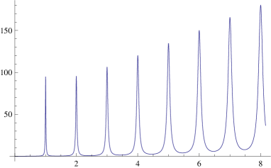
a)   b)

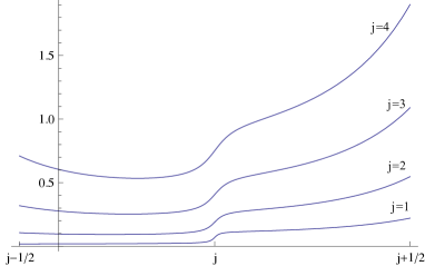
Figure 1. a) shows the effective density of states, computed by summing up the first 15 terms of (6.4), for $\varphi=1/100$. All terms of (6.4) are positive, so the numerical approximation is very good. b) shows the difference between the effective density of states and its approximation by the appropriate Lorentz-profiles $(j+1)(j+2)\ell_{j}/2$, in the intervals $[j-1/2,j+1/2]$, for $j=1,2,3,4$. In both graphs, the units of energy on the $x$-axis are chosen such that the eigenvalues of the uncoupled harmonic oscillator occur at the elements of ${\mathbb{N}}_{0}$.

Figure 1 illustrates the excellent approximation to the effective density of states obtained by the above description, even for the relatively large value $\varphi=1/100$; the physical value for $\varphi$ is about $\alpha^{-3}\approx 0,5\times 10^{-6}$.

With respect to a frequency scale starting at $\omega_{\varphi}$ the peaks at $\omega_{j}$ for $j=1,2,3,\dots$ represent the natural lines of the charged oscillator due to transitions to the ground state (Lyman series). According to (3.10) the distance of two subsequent levels is $\eta\operatorname{cos}\varphi$, which is smaller than $\eta$ in the unperturbed case. The radiative shift (Lamb shift) $\eta-\eta\operatorname{cos}\varphi$ of the first excited state is of second order in $\alpha$.

For an observation of the natural lines the charged oscillator may be brought into contact with black body radiation at the temperature $T=\frac{\hbar}{\rm k\beta}$. This causes additional negative shifts of the excited states depending on $T$ which have to be taken into account. They are determined by the positions of the peaks of $\mu_{\varphi}^{(\beta)}$. For $2T>(\hbar/\rm k)\gamma_{j}$ one readily finds $-\beta\gamma^{2}_{j}/4<\Delta\,\omega_{j}<-\beta\gamma^{2}_{j}/8$.

Our results are in accordance with calculations within QED time–dependent perturbation theory up to first order in the fine-structure constant $\alpha$ (cf. e.g. [5, sec. 5]). The calculations on the radiative cascade of a harmonic oscillator in [7, Exercises 15] confirm also that the shifted levels of the oscillator remain equidistant.

Remark. In our analysis, we have left out the self-interaction term of the field ($A^{2}$)-term). At least Theorem 3.2 can be achieved without this simplification. Actually, in the Göppert-Mayer description this term is absorbed by the coupling, compare [6, IV (B.34)] or [18, (13.124)] and [17, V.15 eq. (15.1), (15.2)]. One is left again with an oscillator model which can be treated in the same way as we do here. The analogous formula to (3.5), without adding any extra renormalization term, is

$$Z(\beta;\gamma)=\left[2\pi\rho\;\prod_{l=1}^{\infty}\left(1+\frac{\rho^{2}}{l^{2}}+\frac{4}{\pi}\sin\varphi\;\left(\gamma-\frac{l}{\rho}\arctan\left(\gamma\frac{\rho}{l}\right)\right)\right)\right]^{-3}.$$

Again the limit $\gamma\to\infty$ does not exist, but this time we do not know how to suitably renormalize this system.

On the other hand, from the well-tested perturbation theory in QED one knows that for many problems concerning the interaction of bound electrons with radiation (e.g. spontaneous and stimulated emission and absorption) the linear part $-epA/m$ of the interaction Hamiltonian yields the main effects (see e.g. [13]).

4. Discretisation of the photon field

Let us now give the proof of Proposition 3.1, and at the same time prepare the proof of Theorem 3.2. In effect, what we give is the reverse procedure to the one that, in the early days of QED, led from the description of the photon field as a collection of independent harmonic oscillators to the Fock space description. So in principle, what we are going to present is well known. However, we are not aware of any place where it is done carefully and in a mathematically satisfactory way, and thus present it in some detail.

Let us start with some properties of the projections $P_{N}$ introduced in (3.3). For locally integrable $f:{\mathbb{R}}^{3}\to{\mathbb{C}}$, and given $j\in J_{N}$, we write

$$\bar{f}_{j}:=\frac{1}{V}\langle 1_{\Lambda_{j}},f\rangle,$$

for the average value of $f$ on $\Lambda_{j}$. Thus, if $f\in L^{2}$ we have

$$P_{N}f(x)=\sum_{j\in J_{N}}\bar{f}_{j}1_{\Lambda_{j}}(x),\quad x\in{\mathbb{R}}^{3}.$$

Lemma 4.1.

Assume $f\in L^{2}({\mathbb{R}}^{3})$, $F\in{\mathcal{F}}$. Then we have:

• As $N\to\infty$, $P_{N}f\to f$ in $L^{2}({\mathbb{R}}^{3})$, and ${\boldsymbol{P}}_{N}F\to F$ in ${\mathcal{F}}$.

• If $f$ is continuous on an open set $B$, then $P_{N}f(x)\to f(x)$ for every $x\in B$.

Proof.

As to (ii), assume without restriction that $f$ is real-valued. Choose $x_{0}\in B$. For all $N$ large enough, we have $\overline{\Lambda}_{j_{0}}\subset B$ for the unique $j_{0}$ such that $x_{0}\in\Lambda_{j_{0}}$. By continuity there are $x_{N},\,x^{\prime}_{N}$ in $\overline{\Lambda}_{j_{0}}$ satisfying $f(x_{N})=\inf f|_{\overline{\Lambda}_{j_{0}}}$ and $f(x^{\prime}_{N})=\sup f|_{\overline{\Lambda}_{j_{0}}}$. Then $P_{N}f(x_{0})=\bar{f}_{j_{0}}\in[f(x_{N}),f(x^{\prime}_{N})]$, whence the assertion.

Now (i) is proved in the standard fashion. Choose $f$ to be the indicator function of a bounded measurable set $B$ at first. Then for each $\varepsilon>0$ there is a continuous functions $g$ with compact support such that $\left\|g-1_{B}\right\|_{L^{2}}<\varepsilon$. Now

$$\left\|P_{N}1_{B}-1_{B}\right\|\;\leqslant\;\left\|P_{N}(g-1_{B})\right\|+\left\|P_{N}g-g\right\|+\left\|g-1_{B}\right\|.$$

The middle term converges to zero by (ii) and dominated convergence, and so the left hand side is bounded by $2\varepsilon$ for all large $N$. This proves the claim for indicators of bounded measurable sets. As the latter are total in $L^{2}$, this proves also the general result about $(P_{N})_{N}$. Finally, the result about $({\boldsymbol{P}}_{N})_{N}$ follows from the fact that second quantisation preserves strong convergence. ∎

It can be checked easily that ${\boldsymbol{P}}_{N}{\mathcal{F}}={\mathcal{F}}(P_{N}L^{2}({\mathbb{R}}^{3}))$, the latter being the Fock space over the image of $P_{N}$. Since $\{h_{j}:\,j\in J_{N}\}$ is a ortonormal basis of $P_{N}L^{2}({\mathbb{R}}^{3})$, we conclude that $\{h_{j_{1}}\hat{\otimes}\ldots\hat{\otimes}h_{j_{n}}:{j_{k}}\in J_{N},\,n\in{\mathbb{N}}_{0}\}$ is a orthonormal basis of ${\boldsymbol{P}}_{N}{\mathcal{F}}$. These basis elements are eigenfunctions of ${\boldsymbol{P}}_{N}H_{\rm f,\sigma}{\boldsymbol{P}}_{N}$, as

$${\boldsymbol{P}}_{N}H_{\rm f,\sigma}\,\,h_{j_{1}}\hat{\otimes}\ldots\hat{\otimes}h_{j_{n}}=\left(\hbar\sum_{i=1}^{n}\bar{\omega}_{j_{i}}\right)\,h_{j_{1}}\hat{\otimes}\ldots\hat{\otimes}h_{j_{n}}.$$

This allows us to transfer the operator $H_{\rm f,N}$ unitarily to an $L^{2}$ space. For $n\in{\mathbb{N}}$ we write for any positive mass parameter $\mu$

$$\psi_{n}(x)=\sqrt{\frac{1}{2^{n}n!}}\left(\frac{\mu\bar{\omega}_{j}}{\pi\hbar}\right)^{1/4}\,{\rm e}^{-\frac{\mu\bar{\omega}_{j}}{2\hbar}x^{2}}\,H_{n}\left(\sqrt{\frac{\mu\bar{\omega}_{j}}{\hbar}}x\right),$$

for the $n$-th Hermite function on ${\mathbb{R}}$. For $j\in J_{N}$ and ${\boldsymbol{j}}:=(j_{1},\ldots,j_{n})\in J_{N}^{n},\;n\in{\mathbb{N}}$ let $n(j,{\boldsymbol{j}})$ denote the number of occurrences of the value $j$ in ${\boldsymbol{j}}$; for $n=0$ set ${\boldsymbol{j}}:=\emptyset,\,h_{\emptyset}:=1\in{\mathbb{C}}$ and $n(j,\emptyset):=0$ for all $j\in J_{N}$. We put

$$h_{{\boldsymbol{j}}}:=h_{j_{1}}\hat{\otimes}\ldots\hat{\otimes}h_{j_{n}}\in{\mathcal{F}}^{(n)}\text{ and }{\boldsymbol{\psi}}_{{\boldsymbol{j}}}:=\bigotimes_{j\in J_{N}}\psi_{n(j,{\boldsymbol{j}})}\,\in L^{2}({\mathbb{R}}^{J_{N}}).$$

Due to symmetrisation, $h_{{\boldsymbol{j}}}$ actually only depends on the occupation numbers $n(j,{\boldsymbol{j}}),\,j\in J_{N}$, and thus it is easy to check that the asignment $\theta(h_{{\boldsymbol{j}}}):={\boldsymbol{\psi}}_{{\boldsymbol{j}}}$ defines an isomorphism from $P_{N}{\mathcal{F}}$ onto $L^{2}({\mathbb{R}}^{J_{N}})$, and that

$$\theta{\boldsymbol{P}}_{N}H_{\rm f,\sigma}\theta^{-1}=\sum_{j\in J_{N}}\left(-\frac{\hbar^{2}}{2\mu}\partial_{x_{\sigma j}}^{2}+\frac{\mu}{2}\bar{\omega}_{j}^{2}x_{\sigma j}^{2}-\frac{\hbar\bar{\omega}_{j}}{2}\right),$$ (4.1)

where $x_{1j}$ and $x_{2j}$ are independent variables. Due to the relation $2xH_{n}(x)=H_{n+1}(x)+2nH_{n-1}(x)$ we have

$$\sqrt{n+1}\psi_{n+1}(x)+\sqrt{n}\psi_{n-1}(x)=\sqrt{\frac{2\mu\bar{\omega}_{j}}{\hbar}}x\psi_{n}(x),$$

and using the definitions of $a^{\ast}(g)$ and $a(g)$, it is tedious but straightforward to check that

$$\theta{\boldsymbol{P}}_{N}H_{\rm I,\sigma}\theta^{-1}=\sqrt{\frac{V\mu}{2\pi^{2}}}\frac{e}{m}\sum_{j\in J_{N}}\sqrt{\bar{\omega}_{j}}(\bar{y}_{\sigma j}\cdot q)x_{\sigma j}\quad\text{with }\;y_{\sigma}:=u_{\sigma}\chi_{c}/\sqrt{\omega}.$$

Thus we find that $H_{N}$ is unitarily equivalent to

$$\tilde{H}_{N}=H_{\rm p}+H_{\rm r,N}+\sum_{j\in J_{N}}\sum_{\sigma=1,2}\left(-\frac{\hbar^{2}}{2\mu}\partial_{x_{\sigma j}}^{2}+\frac{\mu}{2}\bar{\omega}_{j}^{2}x_{\sigma j}^{2}-\frac{\hbar\bar{\omega}_{j}}{2}+\sqrt{\frac{V\mu}{2\pi^{2}}}\frac{e}{m}\sqrt{\bar{\omega}_{j}}(\bar{y}_{\sigma j}\cdot q)x_{\sigma j}\right),$$ (4.2)

acting in $L^{2}({\mathbb{R}}^{3+2J_{N}})$. Here we discretized also the renormalisztion terms

$$H_{\rm r,N}=\sum_{j\in J_{N}}\sum_{\sigma=1,2}V\frac{e^{2}\eta^{2}}{2\pi^{2}m}\;\frac{1}{\bar{\omega}_{j}}(\bar{y}_{\sigma j}\cdot q)^{2}\;-\,\sum_{j\in J_{N}}V\hbar\frac{e^{2}\eta^{2}}{4\pi^{2}m}\,\frac{(\overline{\chi_{c}})_{j}}{\bar{\omega}_{j}^{2}(\bar{\omega}_{j}+\eta)}$$

displaying the contribution to the effective oscillator mass and energy shift by each single photon.

Since $\tilde{H}_{N}$ is the Hamiltonian of a finite dimensional quantum oscillator, its spectrum is discrete and the eigenvalues are of finite multiplicity. Using Lemma 4.1, it is immediate to check (i) and (ii) of Definition 1 for $\rm 1\otimes{\boldsymbol{P}}_{N}\otimes{\boldsymbol{P}}_{N}$, and Proposition 3.1 is proved.

5. The partition function

In this section we will prove Theorems 3.2 and 3.3. We start with a general, useful observation.

5.1. A trace formula for a quantum oscillator

Consider an operator

$$H=\sum_{i=1}^{n}\frac{-\hbar^{2}}{2m_{i}}\,\partial^{2}_{i}+\frac{1}{2}\sum_{i,i^{\prime}=1}^{n}A_{ii^{\prime}}\,X_{i}X_{i^{\prime}}$$ (5.1)

with strictly positive real $n\times n$-matrix $A=(A_{ii^{\prime}})$. $H$ acts in $L^{2}({\mathbb{R}}^{n})$, $\partial_{i}$ are derivative operators with respect to $x_{i}$, and $X_{i}$ are multiplication operators with $x_{i}$. We assume that the mass parameters $m_{i}$ are all positive, and we define the diagonal mass matrix $M:=\mbox{diag}(m_{1},\dots,m_{n})$.

Lemma 5.1.

Let $\lambda_{1},\dots,\lambda_{n}$ be the eigenvalues of $M^{-1/2}\,A\,M^{-1/2}$. Then

$${\operatorname{Tr\,}}\,{\rm e}^{-\frac{\beta}{\hbar}H}\,=\prod_{i=1}^{n}\left(2\sinh(\frac{\beta}{2}\sqrt{\lambda_{i}})\right)^{-1}=\det\left(2\,\sinh\left(\frac{\beta}{2}(M^{-1/2}A\,M^{-1/2})^{\frac{1}{2}}\right)\right)^{-1}=$$

$$\beta^{-n}\det(M^{-1/2}A\,M^{-1/2})^{-\frac{1}{2}}\prod_{l=1}^{\infty}\det\left(I_{n}+(\frac{\beta}{2\pi l})^{2}M^{-1/2}A\,M^{-1/2}\right)^{-1}.$$

Proof. We are going to show that $H$ is unitarily equivalent to

$$\tilde{H}:=\sum_{i=1}^{n}\left(\frac{-\hbar^{2}}{2m_{0}}\,\partial^{2}_{i}+\frac{m_{0}}{2}\lambda_{i}\,X^{2}_{i}\right)$$ (5.2)

with $m_{0}>0$ any mass parameter. Then by Mehler’s formula the first equality holds. The second equality is obvious. The last equality holds true due to the factorization

$$\sinh z=z\prod_{l=1}^{\infty}\left(1+(\frac{z}{\pi l})^{2}\right)$$

valid for all $z\in{\mathbb{C}}$. To show (5.2), we note that any invertible real $n\times n$-matrix $S$ gives rise to a unitary transformation $U$ on $L^{2}({\mathbb{R}}^{n})$ by $Uf:=|\mbox{det}S|^{\frac{1}{2}}\,f\circ S$. We choose $S$ in the following way: Since $M^{-1/2}AM^{-1/2}$ is real symmetric, there exists an orthogonal matrix $O$ such that $OM^{-\frac{1}{2}}AM^{-\frac{1}{2}}O^{T}=\mbox{diag}(\lambda_{1},\dots,\lambda_{n})$. We put $S:=O(\frac{1}{m_{0}}M)^{\frac{1}{2}}$. Then $S$ satisfies

$$SM^{-1}S^{T}=\frac{1}{m_{0}}I_{n},\quad\quad S^{-1T}AS^{-1}=m_{0}\,\mbox{diag}(\lambda_{1},\dots,\lambda_{n}),$$

and from these relations $\tilde{H}=U^{-1}\,H\,U$ follows straightforwardly. $\Box$

5.2. The Partition Functions for $H_{{\rm f},N}$ and $H_{N}$

We will now use Lemma 5.1 in order to compute the partition functions for the discretized systems. Note that from (4.1) and Lemma 5.1 we immediately get

$${\operatorname{Tr\,}}\,{\rm e}^{-\frac{\beta}{\hbar}H_{{\rm f},N}}\,=\,{\rm e}^{\beta\sum_{j\in J_{N}}\bar{\omega}_{j}}\,\prod_{j\in J_{N}}\left(2\sinh(\frac{\beta}{2}\bar{\omega}_{j})\right)^{-2}.$$ (5.3)

Now by (4.2), $\tilde{H}_{N}$ has the form (5.1) up to the constant term

$$-\hbar\sum_{j\in J_{N}}\left(\bar{\omega}_{j}+V\frac{e^{2}\eta^{2}}{4\pi^{2}m}\,\frac{(\overline{\chi}_{c})_{j}}{\bar{\omega}_{j}^{2}(\bar{\omega}_{j}+\eta)}\right).$$

Precisely, the mass matrix $M$ is the diagonal matrix of size $2|J_{N}|+3$, with $\frac{1}{m\eta^{2}}$ as the first three diagonal elements, and $\mu$ as the remaining ones. $A$ is a block matrix of the form

$$A=\left(\begin{matrix}B&B_{1}&B_{2}&\cdots&B_{|J_{N}|}\\ B_{1}^{T}&s_{1}I_{2}&0&\cdots&0\\ B_{2}^{T}&0&s_{2}I_{2}&\ddots&\vdots\\ \vdots&\vdots&\ddots&\ddots&0\\ B_{|J_{N}|}^{T}&0&\cdots&0&s_{|J_{N}|}I_{2}\end{matrix}\right)$$ (5.4)

with $B=\frac{1}{m}I_{3}$ ($I_{j}$ denotes the $j$-dimensional unit matrix), $s_{j}=\mu\bar{\omega}_{j}^{2}$ for $1\;\leqslant\;j\;\leqslant\;|J_{N}|$, and $B_{j}=(v_{1j},v_{2j})\in{\mathbb{R}}^{2\times 3}$, with $v_{\sigma j}=\sqrt{\frac{V\mu}{2\pi^{2}}}\frac{e}{m}\sqrt{\bar{\omega}_{j}}\bar{y}_{\sigma j}$ for $\sigma=1,2$. It is clear that both of the matrices whose determinant appears in the second line of Lemma 5.1 are of the above form, too. We thus need a formula for determinants of matrices of the type (5.4).

Lemma 5.2.

Let $Q$ be a real symmetric $(2L+3)$-dimensional matrix of the form (5.4), where $B$ is 3-dimensional and all $s_{j}\not=0$. Then

$$\emph{det}\,Q=s_{1}^{2}\,\dots\,s_{L}^{2}\;\emph{det}\left(\,B-\sum_{j=1}^{L}\frac{1}{s_{j}}\,B_{j}\,B_{j}^{T}\,\right).$$

Proof. We write $B_{L}=(a,b)$, where $a$ and $b$ are 3-dimensional column vectors. We assume for the moment that $a$ and $b$ are linearly independent. At the end this assumption can be dropped by continuity. Define a $3\times 3$-matrix $X$ by $X^{T}:=(x,y,z)$ with $x:=a\times b,\;y:=b\times x$ and $z:=x\times a$. Then $XB_{L}=|a\times b|^{2}(e_{2},e_{3})$ with $I_{3}=(e_{1},e_{2},e_{3})$ and $X^{-1}=|a\times b|^{-2}(x,a,b)$ hold. The following operations do not change det$\,Q$.

First pass to the equivalent matrix diag$(X,I_{2L})\,Q$ diag$(X^{-1},I_{2L})$. Then the last block in the first block line becomes zero adding $-|a\times b|^{2}/s_{L}$ times the last two lines to the second and third line of the matrix. Expanding now the determinant along the last two columns one obtains the factor $s_{L}^{2}$ times the determinant of a $(2L+1)$-dimensional matrix $Q^{\prime}$. One finds that diag$(X^{-1},I_{2L-2})\,Q^{\prime}$ diag$(X,I_{2L-2})$ arises from $Q$ by canceling the last block line and last block column and replacing $B$ with $B-\frac{1}{s_{L}}B_{L}B_{L}^{T}$. Iterating these operations the result follows. $\Box$

Thus by elementary computations, Lemma 5.1 and Lemma 5.2 yield the following formula for the ratio of the partition functions of the discretised systems:

$$\begin{split}Z_{N}(\beta):=&\frac{{\operatorname{Tr\,}}\,{\rm e}^{-\frac{\beta}{\hbar}H_{N}}\,}{{\operatorname{Tr\,}}\,{\rm e}^{-\frac{\beta}{\hbar}H_{\rm f,N}}\,}=(\beta\eta)^{-3}\,{\rm e}^{\beta\sum_{j\in J_{N}}V\frac{e^{2}\eta^{2}}{4\pi^{2}m}\,\frac{(\overline{\chi}_{c})_{j}}{\bar{\omega}_{j}^{2}(\bar{\omega}_{j}+\eta)}}\,\times\\ &\times\prod_{l=1}^{\infty}\det\left((1+\frac{\eta^{2}}{\nu_{l}^{2}}){\boldsymbol{I}}_{3}+\frac{e^{2}\eta^{2}}{2\pi^{2}m}V\sum_{j\in J_{N}}\sum_{\sigma=1,2}\frac{\bar{y}_{\sigma j}\bar{y}^{T}_{\sigma j}}{\bar{\omega}_{j}(\bar{\omega}_{j}^{2}+\nu_{l}^{2})}\right)^{-1},\end{split}$$ (5.5)

with

$$y_{\sigma}:=\chi_{c}\frac{1}{\sqrt{\omega}}u_{\sigma},\qquad\nu_{l}=\frac{\pi l}{\beta/2}.$$

5.3. The continuum limit

We will now show that in formula (5.5), the limit $N\to\infty$ exists, yielding (3.5). We use the abbreviation

$$S_{l,N}:=\frac{e^{2}\eta^{2}}{2\pi^{2}m}V\sum_{j\in J_{N}}\sum_{\sigma=1,2}\frac{\bar{y}_{\sigma j}\bar{y}^{T}_{\sigma j}}{\bar{\omega}_{j}(\bar{\omega}_{j}^{2}+\nu_{l}^{2})}.$$

Let $\lambda$ denote the Lebesgue measure on ${\mathbb{R}}^{3}$ and put

$$S_{l}:=\frac{e^{2}\eta^{2}}{2\pi^{2}m}\sum_{\sigma=1,2}\int\frac{u_{\sigma}u^{T}_{\sigma}}{\omega^{2}(\omega^{2}+\nu_{l}^{2})}\chi_{c}\,{\rm d}\lambda.$$ (5.6)

Proposition 5.3.

$\lim_{N\to\infty}S_{l,N}=S_{l}$ for each $l\in{\mathbb{N}}$.

Proof.

We will use dominated convergence. Put

$$g_{l,N}:=\sum_{j\in J_{N}}\frac{\bar{y}_{\sigma j}\bar{y}^{T}_{\sigma j}}{\bar{\omega}_{j}(\bar{\omega}_{j}^{2}+\nu_{l}^{2})}1_{\Lambda_{j}}.$$ (5.7)

By the definition of $V$, we have

$$S_{l,N}=\frac{e^{2}\eta^{2}}{2\pi^{2}m}\sum_{\sigma=1,2}\int g_{l,N}{\rm d}\lambda.$$ (5.8)

The functions $y_{\sigma}$, which contain the transverse vector fields, can be chosen to be continuous outside a closed Lebesgue null subset of ${\mathbb{R}}^{3}$ containing the origin. Thus applying Lemma 4.1 (ii) on every factor on the right hand side of (5.7) one deduces that $g_{l,N}$ converges to the integrand in (5.6) almost everywhere.

Now each component of $g_{l,N}$ is bounded by

$$\sum_{j\in J_{N}}\left(\overline{1/\sqrt{\omega}}\right)_{j}^{\,\,2}\frac{1}{\bar{\omega}_{j}\nu_{l}^{2}}1_{\Lambda_{j}}\;\leqslant\;\sum_{j\in J_{N}}\left(\overline{1/\sqrt{\omega}}\right)_{j}^{\,\,4}\frac{1}{\nu_{l}^{2}}1_{\Lambda_{j}},$$

where the inequality is obtained by applying Jensen’s inequality to the convex function $\phi:(0,\infty)\to{\mathbb{R}},\,x\mapsto 1/\sqrt{x}$, yielding $1/\sqrt{\bar{\omega}_{j}}\;\leqslant\;(\,\overline{1/\sqrt{\omega}}\,)_{j}$ for each $j$. Furthermore, we claim that

$$\left(\overline{1/\sqrt{\omega}}\right)_{j}1_{\Lambda_{j}}\;\leqslant\;4\frac{1}{\sqrt{\omega}}1_{\Lambda_{j}}$$ (5.9)

Indeed, in the case $0\in\bar{\Lambda}_{j}$, we replace $\Lambda_{j}$ with the portion of the ball of radius $\sqrt{3}/N$ that lies in the same sector. Then $\Lambda_{j}$ is contained in that set, and

$$\sqrt{c}\left(\overline{1/\sqrt{\omega}}\right)_{j}=\frac{1}{V}\frac{4\pi}{8}\int_{0}^{\sqrt{3}/N}r^{3/2}\,{\rm d}r=\frac{3^{5/4}\pi}{5}N^{1/2}\;\leqslant\;\frac{3^{3/2}\pi}{5\sqrt{r}}\mbox{\quad if }r\leq\sqrt{3}/N,$$

whence the claim in this case. If $0\not\in\bar{\Lambda}_{j}$, we let $(k/N,l/N,m/N)$ be the corner of $\Lambda_{j}$ closest to the origin, and find

$$\sqrt{c}\left(\overline{1/\sqrt{\omega}}\right)_{j}\;\leqslant\;\frac{\sup_{\Lambda_{j}}(1/\sqrt{r})}{\sqrt{r}\inf_{\Lambda_{j}}(1/\sqrt{r})}=\frac{1}{\sqrt{r}}\frac{\sqrt{(k+1)^{2}/N^{2}+(l+1)^{2}/N^{2}+(m+1)^{2}/N^{2}}}{\sqrt{k^{2}/N^{2}+l^{2}/N^{2}+m^{2}/N^{2}}}.$$

The last expression is maximal for $(k,l,m)=(0,0,1)$ and takes the value $\sqrt{6}$ there. Thus (5.9) holds.

Hence every component of $g_{l,N}$ is bounded by $(16/\nu_{l})^{2}\,\omega^{-2}$, which is locally integrable. This finishes the proof. ∎

A similar, but easier proof shows that

$$\lim_{N\to\infty}\sum_{j\in J_{N}}V\frac{e^{2}\eta^{2}}{4\pi^{2}m}\,\frac{(\overline{\chi}_{c})_{j}}{\bar{\omega}_{j}^{2}(\bar{\omega}_{j}+\eta)}=\frac{e^{2}\eta^{2}}{4\pi^{2}m}\int\frac{\chi_{c}}{\omega^{2}(\omega+\eta)}{\rm d}\lambda.$$ (5.10)

The integrals appearing in (5.10) and (5.6) can be calculated. We have

$$\int\frac{\chi_{c}}{\omega^{2}(\omega+\eta)}{\rm d}\lambda=\frac{4\pi}{c^{3}}\ln(1+\tfrac{Cc}{\eta}).$$

Together with the prefactor, and comparing with the definitions of $\sin\varphi$, $\rho$ and $\gamma$, we obtain the exponent in (3.5). For (5.6), note first that $\sum_{\sigma=1,2}u_{\sigma}u_{\sigma}^{T}={\boldsymbol{I}}_{3}-\frac{1}{|k|^{2}}kk^{T}$ follows from the orthonormality of $u_{1}$, $u_{2}$ and $k/|k|$. Thus for each component of $\sum_{\sigma=1,2}\int\frac{u_{\sigma}u^{T}_{\sigma}}{\omega^{2}(\omega^{2}+\nu_{l}^{2})}\chi_{c}\,{\rm d}\lambda$, the angular part can be calculated, and is found to be equal to $\frac{8\pi}{3}$. Then

$$\sum_{\sigma=1,2}\int\frac{u_{\sigma}u^{T}_{\sigma}}{\omega^{2}(\omega^{2}+\nu_{l}^{2})}\chi_{c}\,{\rm d}\lambda=\frac{8\pi}{3c^{3}\nu_{l}}\arctan\left(\tfrac{cC}{\nu_{l}}\right){\boldsymbol{I}}_{3}.$$

Taking the prefactor into account and computing the now trivial determinant gives the $l$-th factor of the infinite product in (3.5).

The final step is to justify the exchange of the infinite product with the limit $N\to\infty$. To this end, we write, for each $l\in{\mathbb{N}}$,

$$M_{l,N}:=\frac{\eta^{2}}{\nu_{l}^{2}}{\boldsymbol{I}}_{3}+S_{l,N},\qquad M_{l}:=\lim_{N\to\infty}M_{l,N}=\frac{\eta^{2}}{\nu_{l}^{2}}{\boldsymbol{I}}_{3}+S_{l}.$$

Lemma 5.4.

We have

$$\lim_{N\to\infty}\prod_{l=1}^{\infty}\det({\boldsymbol{I}}_{3}+M_{l,N})=\prod_{l=1}^{\infty}\det({\boldsymbol{I}}_{3}+M_{l}).$$

Proof.

By the continuity of the exponential function, it will suffice to prove the result for the logarithms. Then the quantity of interest is given by

$$\ln\left(\prod_{l=1}^{\infty}\det({\boldsymbol{I}}_{3}+M_{l,N})\right)=\sum_{l=1}^{\infty}\ln(\det({\boldsymbol{I}}_{3}+M_{l,N})).$$

Since by continuity

$$\lim_{N\to\infty}\ln(\det({\boldsymbol{I}}_{3}+M_{l,N}))=\ln(\det({\boldsymbol{I}}_{3}+M_{l}))$$

for each $l\in{\mathbb{N}}$, the result will follow by dominated convergence.

At the end of the proof of Proposition 5.3 we have seen that $S_{l,N}$ is bounded by ${\rm constant}/l^{2}$ uniformly in $N$. Thus so is $\|M_{l,N}\|$ and hence its three eigenvalues. It follows that $|\det({\boldsymbol{I}}_{3}+M_{l,N}))-1|\;\leqslant\;{\rm constant}/l^{2}$ and therefore

$$|\ln(\det({\boldsymbol{I}}_{3}+M_{l,N}))|\;\leqslant\;{\rm constant}/l^{2}$$

uniformly in $N$. ∎

We have thus proved Theorem 3.2.

5.4. Removing the ultraviolet limit

We now investigate the limit $\gamma\to\infty$ in (3.5). Clearly, what we need to show is the convergence of

$$f(\gamma):=-2\sin\varphi\;\rho\ln(1+\gamma)+\sum_{l=1}^{\infty}\ln(1+h_{l}(\gamma)),$$

where

$$h_{l}(\gamma)=\frac{\rho^{2}}{l^{2}}+\frac{4}{\pi}\sin\varphi\,\arctan\left(\frac{\gamma\rho}{l}\right).$$

We first note that

$$0<h_{l}(\gamma)<\frac{\rho^{2}}{l^{2}}\left(1+\frac{4}{\pi}\gamma\sin\varphi\right)$$ (5.11)

$$0<h_{l}(\gamma)\nearrow h_{l}:=\frac{\rho^{2}}{l^{2}}+2\frac{\rho}{l}\sin\varphi\text{ \;monotonically for }\gamma\nearrow\infty.$$ (5.12)

By (5.11), $(h_{l}(\gamma))$ is summable for all $\gamma$, and thus

$$f(\gamma)=\left(\sum_{l=1}^{\infty}h_{l}(\gamma)-2\sin\varphi\;\rho\ln(1+\gamma)\right)+\sum_{l=1}^{\infty}\left(\ln\big{(}1+h_{l}(\gamma)\big{)}-h_{l}(\gamma)\right).$$ (5.13)

We now use the formula

$$\mathcal{C}=\lim_{s\to\infty}\left[\frac{2}{\pi}\sum_{l=1}^{\infty}\frac{1}{l}\arctan(\frac{s}{l})\,-\ln s\right]$$ (5.14)

for the Euler/Mascheroni constant $\mathcal{C}$. The first bracket above is then equal to

$$\sum_{l=1}^{\infty}\frac{\rho^{2}}{l^{2}}+2\sin\varphi\;\rho\left(\ln\rho+\ln\left(\tfrac{\gamma}{1+\gamma}\right)+\frac{2}{\pi}\sum_{l=1}^{\infty}\frac{1}{l}\arctan\left(\tfrac{\rho\gamma}{l}\right)-\ln(\rho\gamma)\right),$$

and by (5.14) converges to $\sum_{l=1}^{\infty}\frac{\rho^{2}}{l^{2}}+2\sin(\varphi)\rho({\mathcal{C}}+\ln(\rho))$. The last sum in (5.13) converges to $\sum_{l=1}^{\infty}\left(\ln\big{(}1+h_{l}\big{)}-h_{l}\right)$ by (5.12) and monotone convergence, since $\ln(1+x)-x$ is monotone decreasing. Combining these two results, we obtain

$$\begin{split}f&:=\lim_{\gamma\to\infty}f(\gamma)=2\sin\varphi\;\rho({\mathcal{C}}+\ln(\rho))+\sum_{l=1}^{\infty}\left(\ln\big{(}1+h_{l}\big{)}-2\frac{\rho}{l}\sin\varphi\right)\\ &=2\sin\varphi\;\rho({\mathcal{C}}+\ln(\rho))+\ln\left(\prod_{l=1}^{\infty}(1+h_{l})\,{\rm e}^{-2\frac{\rho}{l}}\,\sin\varphi\right).\end{split}$$

Taking into account that $1+h_{l}=(1+\frac{\rho}{l}i\,{\rm e}^{-i\varphi}\,)(1+\frac{\rho}{l}i\,{\rm e}^{i\varphi}\,)$, and writing $2i\sin\varphi=\,{\rm e}^{i\varphi}\,-\,{\rm e}^{-i\varphi}\,$, we find

$$\,{\rm e}^{f}\,=\frac{1}{\rho^{2}}\,{\rm e}^{2\rho\ln(\rho)\sin\varphi}\,\left|\rho\,{\rm e}^{{\mathcal{C}}\rho\,i\,{\rm e}^{-{\rm i}\varphi}\,}\,\prod_{j=1}^{\infty}\left(1+\frac{\rho}{l}i\,{\rm e}^{-{\rm i}\varphi}\,\right)\,{\rm e}^{\frac{\rho}{l}i\,{\rm e}^{-{\rm i}\phi}\,}\,\right|^{2}.$$

Using the representation

$$\Gamma(z)^{-1}=z\,{\rm e}^{\mathcal{C}z}\,\prod_{l=1}^{\infty}(1+\frac{z}{l})\,{\rm e}^{-\frac{z}{l}}\,\quad\text{ for }\operatorname{Re}\,z>0,$$

for the Gamma function on the right half-plane, we arrive at (3.6).

6. The effective measure of states

In this section, we investigate the inverse Laplace transform of $Z(\beta)$. As a first step, we prove the second part of Theorem 3.3.

6.1. Complete monotonicity

By Bernstein’s theorem, a function $f$ on $[0,\infty[$ is the Laplace transform of a positive Borel measure if and only if it is completely monotone (c.m.), i.e. $(-1)^{n}\partial_{x}^{n}f(x)\;\geqslant\;0$ for all $x\;\geqslant\;0$. To show that $Z(\beta)$ is c.m., we use (3.6) in order to get

$$\frac{1}{3}\ln Z(\beta)=\ln\rho-\ln(2\pi)-2\sin\varphi\;\rho\ln\rho+\ln\Gamma(\rho\,i\,{\rm e}^{-{\rm i}\varphi}\,)+\ln\overline{\Gamma(\rho\,i\,{\rm e}^{-{\rm i}\varphi}\,)}.$$

We now use Binet‘s formula

$$\ln\Gamma(z)=\int_{0}^{\infty}\frac{\,{\rm e}^{-tz}\,}{t}\left(\frac{1}{1-\,{\rm e}^{-t}\,}-\frac{1}{t}-\frac{1}{2}\right)\,{\rm d}t+\frac{\ln(2\pi)}{2}+(z-\tfrac{1}{2})\ln(z)-z,$$

valid for ${\operatorname{Re\,}}(z)>0$. Since $\ln(\bar{z})=\overline{\ln(z)}$ for all $z\in{\mathbb{C}}$, we obtain

$$\begin{split}\ln Z(\beta)=\int_{0}^{\infty}\,{\rm e}^{-t\rho}\,\,g(t)\,{\rm d}t\,\;-\,t_{\varphi}\,\rho\end{split}$$ (6.1)

with

$$g(t):=\frac{6}{t}\,{\operatorname{Re\,}}\left(\frac{1}{1-\,{\rm e}^{-\tau}\,}-\frac{1}{\tau}-\frac{1}{2}\right),\quad\tau:=i\,{\rm e}^{-i\varphi}\,t,\quad t_{\varphi}:=6\big{(}\sin\varphi+(\frac{\pi}{2}-\varphi)\cos\varphi\big{)}.$$

Below we will show that $g(t)\;\geqslant\;0$ for all $t\;\geqslant\;0$. This immediately implies that the first term on the right hand side of (6.1) is c.m. Since the product of two c.m. functions is c.m.  also $\exp(f)$ is c.m. if $f$ is. Thus $Z(\beta)$ is c.m. as the product of $\exp(\int_{0}^{\infty}\,{\rm e}^{-t\rho}\,g(t)\,{\rm d}t)$ and the the clearly c.m. function $\exp(-t_{\varphi}\rho)$. The claim $g(t)\;\geqslant\;0$ follows from

Lemma 6.1.

For all $w\in{\mathbb{C}}$ with ${\operatorname{Re\,}}(w)>0$ we have

$$h(w):={\operatorname{Re\,}}\left(\frac{1}{1-\,{\rm e}^{-w}\,}-\frac{1}{w}-\frac{1}{2}\right)\;\geqslant\;0.$$

Equality holds if an only if ${\operatorname{Re\,}}(w)=0$.

Proof.

We write $w=u+{\rm i}v$. If $u=0$, then $h({\rm i}v)=\frac{1-\cos v}{1-2\cos v+1}-\frac{1}{2}=0$. For $u>0$, a direct calculation yields

$$\begin{split}h(z)&=\frac{(u^{2}+v^{2})(1-\,{\rm e}^{-2u}\,)-2u(1+\,{\rm e}^{-2u}\,-2\,{\rm e}^{-u}\,\cos v)}{2(1-2\,{\rm e}^{-u}\,\cos v+\,{\rm e}^{-2u}\,)(u^{2}+v^{2})}=\\ &=\frac{(u^{2}+v^{2})\sinh(u)-2u(\cosh(u)-\cos(v))}{2(u^{2}+v^{2})(\cosh(u)-\cos(v))}\end{split}$$

with nonnegative denominator. We need to show that the numerator $r(u,v)$ is positive if $u>0$. By symmetry it suffices to treat $v\;\geqslant\;0$. Take first $v=0$. Then $\partial_{u}(r(u,0)/u)=u\cosh u-\sinh u$, which at $u=0$ equals $0$. Since $\partial_{u}^{2}(r(u,0)/u)=u\sinh u>0$, $u\mapsto r(u,0)>0$ for $u>0$. Thus the result holds if $\partial_{v}r(u,v)=2(v\sinh u-u\sin v)$ is nonnegative for all $u>0,\,v>0$. But this is clearly true, since $(\sinh u)/u>1>(\sin v)/v$ for all $u,v\neq 0$. ∎

6.2. Analytic continuation

Here we prove Theorem 3.5. Let us define

$$Y(\rho):=Z(\beta)\,{\rm e}^{t_{\varphi}\rho}\,.$$

Since $\rho=\frac{\eta\beta}{2\pi}$, the inverse Laplace transforms of $Y(\rho)$ and $Z(\beta)$ are related by translation and scaling. The key observation is that, due to (6.1), $Y$ is itself the exponential of a Laplace transform,

$$Y(\rho)=\exp\mathfrak{L}g(\rho)=1+\sum_{n=1}^{\infty}\frac{1}{n!}\mathfrak{L}g^{\ast n}(\rho).$$ (6.2)

Above, $\mathfrak{L}$ denotes the Laplace transformation, and

$$h\ast k\,(x)=\int_{0}^{x}h(t)k(x-t)\,{\rm d}t$$ (6.3)

is the convolution of functions supported on $[0,\infty[$. Since $g$ is bounded on compact intervals and nonnegative, the final sum in (6.2) converges uniformly on compact intervals. Let us define

$$\varrho:=\sum_{n=1}^{\infty}\frac{1}{n!}\,g^{\ast n}.$$ (6.4)

By Lemma 6.1, all terms of the above sum are positive. Thus $\mathfrak{L}\varrho=Y-1$ holds by monotone convergence, and the uniqueness of Laplace transforms shows $\mathfrak{L}^{-1}Y=\delta_{0}+\varrho$. Moreover, a direct calculation shows that $g(t)\to\frac{1}{2}\sin\varphi$ as $t\to 0$. Thus the same holds for $\varrho$, and we have shown the first part of Theorem 3.5, with $\phi(\omega)=\frac{2\pi}{\eta}\varrho\big{(}\tfrac{2\pi}{\eta}(\omega-\omega_{\varphi})\big{)}$ for $\omega\geq\omega_{\varphi}$ and zero else.

We now investigate the analytic continuation of $\varrho$. First note that the analytic continuation of $g$ is given by

$$g(z)=\frac{3}{z}\left[\frac{1}{1-\exp(-{\rm i}\,{\rm e}^{-{\rm i}\varphi}\,z)}+\frac{1}{1-\exp({\rm i}\,{\rm e}^{{\rm i}\varphi}\,z)}-\frac{2\sin\varphi}{z}-1\right].$$

Lemma 6.2.

$g$ is a meromorphic function on ${\mathbb{C}}$ with simple poles at the zeros of the denominators

$$q_{j}=2\pi j\,{\rm e}^{-{\rm i}\varphi}\,\quad\text{ and }\quad\overline{q_{j}}=2\pi j\,{\rm e}^{{\rm i}\varphi}\,,\qquad j\in{\mathbb{Z}}\setminus\{0\}.$$

The residues are  $\operatorname{Res}(g;q_{j})=\frac{3{\rm i}}{2\pi j}$,  $\operatorname{Res}(g;\overline{q_{j}})=\frac{-3{\rm i}}{2\pi j}$.

The proof is routine. Note only that we have seen already above that the common zero $z=0$ of the denominators actually is a regular point of $g$.

Let us now consider the analytic continuation of the convolutions. Define ${\mathcal{P}}:=\{z:\,z=q_{j}\mbox{ or }z=\overline{q_{j}}\text{ for all }j\in{\mathbb{Z}}\setminus\{0\}\}$ and ${\mathcal{S}}:=\{z:\,z=s\,{\rm e}^{\pm i\varphi}\,\mbox{ \;for real\, }s\mbox{\, with\, }|s|\geq 2\pi\}$. For brevity use $A({\mathcal{S}},{\mathcal{P}})$ to denote the set of functions $f$ that are analytic on ${\mathbb{C}}\setminus{\mathcal{S}}$ such that the components of ${\mathcal{S}}\setminus{\mathcal{P}}$ are cuts for $f$ emanating from the points of ${\mathcal{P}}$. Analytic functions on ${\mathbb{C}}\setminus{\mathcal{P}}$ are elements of $A({\mathcal{S}},{\mathcal{P}})$. — For any function $f$ and any subset $K$ of ${\mathbb{C}}$ let $\|f\|_{K}$ denote the supremum of $|f|$ on $K$.

Lemma 6.3.

Let $h\in A({\mathcal{S}},{\mathcal{P}})$ and let $k$ be analytic on ${\mathbb{C}}\setminus{\mathcal{P}}$. For $z\in{\mathbb{C}}\setminus{\mathcal{S}}$ set

$$F(z):=\int_{0}^{z}h(\zeta)k(z-\zeta)\,{\rm d}\zeta$$

integrating along the straight line joining $0$ and $z$. Then $F\in A({\mathcal{S}},{\mathcal{P}})$ and $F$ is an analytic continuation of $h\ast k$ as defined in (6.3). Let $K$ be any compact subset of ${\mathbb{C}}\setminus{\mathcal{S}}$ and let $\tilde{K}$ denote the union of all straight lines joining the origin with some point of $K$. Then $\|F\|_{K}\leq\|id\|_{K}\,\|h\|_{\tilde{K}}\,\|k\|_{\tilde{K}}$.

Proof.

Plainly, $F$ agrees with $h\ast k$ on the real axis and is differentiable at all $z\in{\mathbb{C}}\setminus{\mathcal{S}}$. Hence F is an analytic continuation of $h\ast k$ on ${\mathbb{C}}\setminus{\mathcal{S}}$. — We turn to the analytic continuation $\tilde{F}$ of $F$, e.g., from above across the cut between the points $q_{j}$ and $q_{j+1}$ with $j\in{\mathbb{N}}$. Let $z\in{\mathcal{S}}_{1}:=\{z:\,z=s\,{\rm e}^{-{\rm i}\varphi}\,\mbox{ \;for }s\geq 2\pi\}$ be between $q_{j}$ and $q_{j+1}$. Join the points $0$ and $z$ along ${\mathcal{S}}_{1}$ but avoiding $q_{l}$, respectively $z-q_{l}$, for $l=1,\dots,j$, by making a small detour above, respectively below, ${\mathcal{S}}_{1}$. By analogous curves $\gamma_{z}$ one joins $0$ to $z$ for every $z$ in the open disk $D$ centered at $\frac{1}{2}(q_{j}+q_{j+1})$ with radius $\pi$. Let $\tilde{h}$ be an analytic continuation of $h$ from above ${\mathcal{S}}_{1}$ across the cuts along ${\mathcal{S}}_{1}$. Then

$$\tilde{F}(z):=\int_{\gamma_{z}}\tilde{h}(\zeta)k(z-\zeta)\,{\rm d}\zeta$$

defines an analytic function on $D$. It extends $F$, since for $z\in D$ above ${\mathcal{S}}_{1}$ the closed curve composed by $\gamma_{z}$ and the straight line from $z$ to $0$ does not contain any singularity of $\zeta\to\tilde{h}(\zeta)k(z-\zeta)$. — The remainder is obvious. ∎

By the lemma, $g^{\ast n}\in A({\mathcal{S}},{\mathcal{P}})$ for all $n\in{\mathbb{N}}$. Moreover, $\|g^{\ast n}\|_{K}\leq\|\rm{id}\|_{K}^{n-1}\,\|g\|_{\tilde{K}}^{n}$. Obviously, a similar estimate holds more generally for the analytic continuations $\tilde{F}$ of $F$ on compact $K\subset\operatorname{dom}\tilde{F}$. Hence the series in (6.4) converges uniformly on compact sets implying that the limiting function belongs to $A({\mathcal{S}},{\mathcal{P}})$. This proves the second part of Theorem 3.5 when taking into account that the translation and scaling takes $q_{j}$ into $p_{j}$.

Let us comment on the cuts of $F$ from Lemma 6.3. Even if $h$ and $k$ are analytic on ${\mathbb{C}}\setminus{\mathcal{P}}$ with poles at points of ${\mathcal{P}}$, the convolution $F$ may have cuts. More precisely, e.g., if $z$ lies on the cut between $q_{j}$ and $q_{j+1}$ with $j\in{\mathbb{N}}$ then

$$F_{+}(z)-F_{-}(z)=-2\pi\,{\rm i}\sum_{l=1}^{j}\left[k(z-q_{l})\,\operatorname{Res}(h;q_{l})+h(z-q_{l})\,\operatorname{Res}(k;q_{l})\right]$$

where $F_{+}(z)$ and $F_{-}(z)$ denote the limit values of $F$ at $z$ approaching $z$ from above and from below the cut, respectively. This is an immediate consequence of Residue Theorem integrating the meromorphic function $\zeta\to M_{z}(\zeta):=h(\zeta)k(z-\zeta)$ along the simply closed curve, which is symmetric with respect to ${\mathcal{S}}_{1}$ and which joins $0$ to $z$ by $\gamma_{z}$. — In case of $F=g\ast g$ the above formula yields the jump function

$$F_{+}(z)-F_{-}(z)=\sum_{l=1}^{j}\,\frac{6}{l}g(z-2\pi\,l\,{\rm e}^{-i\varphi}\,).$$

6.3. Analysis of the singularities

Here we prove Theorem 3.6. Again it suffices to analyse $\varrho$ (6.4) instead of $\phi$ as $\phi(\omega)=\frac{2\pi}{\eta}\varrho\big{(}\tfrac{2\pi}{\eta}(\omega-\omega_{\varphi})\big{)}$ for $\omega\geq\omega_{\varphi}$. We refer to the analytic continuations of the convolutions $g^{\ast n}$ and of $\varrho$ defined in Section 6.2.

First note the following formula for $z=s\,{\rm e}^{{\rm i}\chi}\,$ with $s>0$ and $|\chi|<\varphi$

$$\int_{0}^{z}\frac{1}{\zeta-q_{j}}\frac{1}{z-\zeta-q_{k}}\,{\rm d}\zeta=\frac{-2\pi{\rm i}}{z-q_{j}-q_{k}}+\frac{\ln(z-q_{j})-\ln q_{j}+\ln(z-q_{k})-\ln q_{k}}{z-q_{j}-q_{k}},$$ (6.5)

which follows from the partial fraction expansion $\frac{1}{\zeta-q_{j}}\frac{1}{z-\zeta-q_{k}}=\frac{1}{z-q_{j}-q_{k}}\left(\frac{1}{\zeta-q_{j}}+\frac{1}{z-\zeta-q_{k}}\right)$ evaluating the primitives $\ln(\zeta-q_{j})$ and $-\ln(z-\zeta-q_{k})$ of $(\zeta-q_{j})^{-1}$ and $(z-\zeta-q_{k})^{-1}$, respectively. Note that the second term in (6.5) is regular at $q_{j}+q_{k}=q_{j+k}$. Next let us define recursively the coefficients

$$c_{j1}=\tilde{c}_{j1}=\frac{3}{j},\qquad c_{j,n+1}=\sum_{k=1}^{j-1}c_{k1}c_{j-k,n},\quad\tilde{c}_{j,n+1}=-\sum_{k=1}^{j-1}\tilde{c}_{k1}\tilde{c}_{j-k,n}$$ (6.6)

for all $j,n\in{\mathbb{N}}$, where the void sums for $j=1$ are zero. Set

$$s_{jn}(z):=\frac{-c_{jn}}{2\pi{\rm i}(z-q_{j})},\qquad\tilde{s}_{jn}(z):=\frac{-\tilde{c}_{jn}}{2\pi{\rm i}(z-q_{j})}.$$

In the following, we will concentrate on the forth quadrant of ${\mathbb{C}}$. Subsequently it will be easy to extend the result to the right half-plane. Fix $N\in{\mathbb{N}}$ and let $z=s\,{\rm e}^{{\rm i}\chi}\,$ with $0\leq s\leq 2\pi N$ and  $-\frac{\pi}{2}\leq\chi\leq 0$.

Proposition 6.4.

Then

$$g^{\ast n}(z)=\sum_{j=1}^{N}s_{jn}(z)+L_{n}(z)\qquad\text{for }\,|\chi|<\varphi,$$

$$g^{\ast n}(z)=\sum_{j=1}^{N}\tilde{s}_{jn}(z)+\tilde{L}_{n}(z)\qquad\text{for }|\chi|>\varphi$$

hold with $|L_{n}(z)|$ and $|\tilde{L}_{n}(z)|$ bounded by $A^{n}(1+\big{|}\ln\sin|\varphi-|\chi||\big{|}^{s})$ for some constant $A$.

Proof.

We proceed by induction. The statement for $n=1$ follows from Lemma 6.2; indeed, subtracting from $g$ the first order poles at $q_{1},\dots,q_{N}$ leaves a bounded function $L_{1}$. Let us now assume that $g^{\ast n}$ has the asserted decomposition and consider the case $|\chi|<\varphi$. Then

$$\begin{split}g^{\ast(n+1)}(z)&=\sum_{j,k=1}^{N}\int_{0}^{z}s_{j1}(\zeta)s_{kn}(z-\zeta)\,{\rm d}\zeta\\ &+\sum_{j=1}^{N}\int_{0}^{z}\left(s_{j1}(\zeta)L_{n}(z-\zeta)+s_{jn}(\zeta)L_{1}(z-\zeta)\right)\,{\rm d}\zeta.\end{split}$$ (6.7)

By (6.5) we find

$$\int_{0}^{z}s_{j1}(\zeta)s_{kn}(z-\zeta)\,{\rm d}\zeta=\frac{-c_{j1}c_{kn}}{2\pi{\rm i}(z-q_{j+k})}+L_{jkn}(z),$$ (6.8)

where $L_{jkn}$ is regular at $q_{j+k}$. The first term above contributes to $s_{j+k,n+1}$. We will show below that none of the remaining terms entering $g^{\ast(n+1)}$ has any first order poles, and thus by collecting all terms with $j+k=m$ we obtain the recursive equation for $c_{m,n+1}$. The calculation for $\tilde{s}_{jn}$, i.e. for $|\chi|>\varphi$, is very similar. The only difference is that the residue of the pole at $q_{j+k}$ in (6.5) is $2\pi{\rm i}$ instead of $-2\pi{\rm i}$, a difference which is due to two jumps of $2\pi{\rm i}$ of the logarithmic terms at the cut along the negative real axis. This gives the additional minus sign in the recursion for $\tilde{c}_{jn}$.

We turn to $L_{jkn}$. As mentioned above, there is no singularity at $q_{j+k}$. There are two logarithmic singularities at $q_{j}$ and $q_{k}$. Other than that, $L_{jkn}$ is bounded. Set $\delta:=|\varphi-|\chi||$ and $h(\delta):=|\ln(\sin\delta)|$. Then $|L_{jkn}(z)|\;\leqslant\;c_{j1}c_{kn}\,K(1+h(\delta))$ for some constant $K$. It is immediate from (6.6) that $c_{jn}=0$ for $j<n$. Thus there exists some constant $B$, independent of $n$, such that

$$\sum_{j,k=1}^{N}|L_{jkn}(z)|\;\leqslant\;B\,(1+h(\delta)).$$

Now we tackle the second line of (6.7). By the induction hypothesis, $|L_{n}(z)|\;\leqslant\;A^{n}(1+h(\delta)^{s})$. Thus

$$\begin{split}I_{jn}(z)&:=\left|\int_{0}^{z}s_{j1}(\zeta)L_{n}(z-\zeta)\,{\rm d}\zeta\right|\;\leqslant\;\\ &\;\leqslant\;A^{n}h(\delta)^{s}\int_{0}^{s}|s_{j1}(y\,{\rm e}^{{\rm i}\chi}\,)|\,h(\delta)^{-y}\,{\rm d}y+A^{n}\int_{0}^{s}|s_{j1}(y\,{\rm e}^{{\rm i}\chi}\,)|\,{\rm d}y.\end{split}$$

For $s\leq\pi$, the integrands on the right hand side above are bounded, and hence $I_{jn}(z)\;\leqslant\;$ $DA^{n}(1+h(\delta)^{s})$ for some constant $D$. For $s>\pi$, we decompose the domain of integration into $y\leq\pi$ and $\pi<y\leq s$. On the first interval, the integrands are bounded with the same result as above. On the second interval, we replace $h(\delta)^{-y}$ by $h(\delta)^{-\pi}$. The integral over $s_{1j}$ alone is clearly bounded by $E(1+h(\delta))$ for some constant $E$, and we estimate crudely

$$\sum_{j=1}^{N}I_{jn}(z)\;\leqslant\;3NA^{n}(D+E)(1+h(\delta)^{s}).$$

Finally, since $L_{1}$ is bounded, we have

$$\sum_{j=1}^{N}\left|\int_{0}^{z}s_{jn}(\zeta)L_{1}(z-\zeta)\,{\rm d}\zeta\right|\;\leqslant\;F(1+h(\delta)),$$

where the constant $F$ does not depend on $n$. Altogether, we find $|L_{n+1}(z)|\;\leqslant\;3NA^{n}(D+E+B+F)(1+h(\delta)^{s})$. Clearly, setting $A=3N(1+D+E+B+F)$, this is bounded by $A^{n+1}(1+h(\delta)^{s})$. ∎

In order to extend this result to the right half-plane one has to take account of the poles $\overline{q}_{j}$ of $g$, too. This amounts in replacing $s_{jn}(z)$ by $s_{jn}(z)+\overline{s_{jn}(\overline{z})}$. Let $M_{n}$ denote the remainder in place of $L_{n}$. It satisfies the same kind of estimate with some new constant $A$. Using (6.4) and the fact that $c_{jn}=0$ for $j<n$, we now have

$$\varrho(z)=\sum_{j=1}^{N}\left(\sum_{n=1}^{j}\frac{c_{jn}}{n!}\right)\left(\frac{-1}{2\pi{\rm i}(z-q_{j})}+\frac{1}{2\pi{\rm i}(z-\overline{q}_{j})}\right)+M(z)$$

with $M:=\sum_{n=1}^{\infty}\frac{1}{n!}M_{n}$ and $|M(z)|\leq\,{\rm e}^{A}\,(1+h(\delta)^{s})$ for $-\varphi<\chi<\varphi$. The same formula with $\tilde{c}_{jn}$ and $\tilde{M}$ holds for $|\chi|>\varphi$. Obviously $h(\delta)^{s}$ can be replaced by $|\ln\delta|^{2\pi N}$.

Proposition 6.5.

Define $c_{jn}$ and $\tilde{c}_{jn}$ as in (6.6). Then, for all $j\in{\mathbb{N}}$,

$$\sum_{n=1}^{j}\frac{c_{jn}}{n!}=\binom{j+2}{2},\qquad\text{and}\qquad\sum_{n=1}^{j}\frac{\tilde{c}_{jn}}{n!}=(-1)^{j+1}\binom{3}{j}\quad\text{ if }j\;\leqslant\;3,\text{and }0\text{ otherwise.}$$

Proof.

We introduce the generating functions $F_{n}(x)=\sum_{j=1}^{\infty}c_{jn}x^{j}$. Then, $F_{1}(x)=\sum_{j=1}^{\infty}\frac{3}{j}x^{j}=-3\ln(1-x)$, and $F_{n}=F_{1}^{\,n}$. The last statement follows from

$$F_{1}(x)F_{n}(x)=\sum_{j=1}^{\infty}\left(\sum_{k=1}^{j-1}c_{k1}c_{j-k,n}\right)x^{j}=\sum_{j=1}^{\infty}c_{j,n+1}x^{j}=F_{n+1}(x).$$

Now recall that $c_{jn}=0$ for $j<n$. Then

$$\begin{split}\sum_{n=1}^{\infty}\frac{c_{jn}}{n!}&=\frac{1}{j!}\partial_{x}^{j}\sum_{n=1}^{\infty}\frac{F_{1}(x)^{n}}{n!}\Big{|}_{x=0}=\frac{1}{j!}\partial_{x}^{j}\left(\,{\rm e}^{F_{1}(x)}\,-1\right)\Big{|}_{x=0}=\\ &=\frac{1}{j!}\partial_{x}^{j}\,{\rm e}^{-3\ln(1-x)}\,\Big{|}_{x=0}=\frac{1}{j!}\partial_{x}^{j}\frac{1}{(1-x)^{3}}\Big{|}_{x=0}=\binom{j+2}{2}.\end{split}$$

For the generating function $\tilde{F}_{n}$ of $(\tilde{c}_{jn})$, a similar calculation leads to $\tilde{F}_{n}=(-1)^{n+1}\tilde{F}_{1}^{\,n}$ with $\tilde{F}_{1}=F_{1}$. Thus, as above,

$$\sum_{n=1}^{\infty}\frac{\tilde{c}_{jn}}{n!}=-\frac{1}{j!}\partial_{x}^{j}\,{\rm e}^{3\ln(1-x)}\,\Big{|}_{x=0}=-\frac{1}{j!}\partial_{x}^{j}(1-x)^{3}\Big{|}_{x=0}.$$

This equals $3$ for $j=1$, $-3$ for $j=2$, $1$ for $j=3$, and zero otherwise, as was claimed. ∎

The stated analyticity properties of $h_{N}(z)$ and $\tilde{h}_{N}(z)$ from Theorem 3.6 are true by the fact that both $\phi$ (cf. Theorem 3.5) and $\ell_{j}$ possess them. This concludes the proof of Theorem 3.6.

7. Appendix

Here we show that Definition 2 of a resonance is equivalent to that given e.g. in [16, XII.6]. We start with a Lemma that connects the analyticity of a measure’s density with properties of its Stieltjes transform.

Let $\mu$ be a finite Borel measure on $[0,\infty[$ and $f:=\tilde{\mu}$ its Stieltjes transform. Note that $f$ is holomorphic on ${\mathbb{C}}\setminus[0,\infty[$ and satisfies $\overline{f(z)}=f(\overline{z})$. We recall the classical inversion formula valid for $t\geq 0$:

$$\mu([0,t])=\operatorname{lim}_{\delta\to 0+}\operatorname{lim}_{\epsilon\to 0+}\frac{1}{\pi}\int_{0}^{t+\delta}\operatorname{Im}\,f(s+{\rm i}\epsilon)\,{\rm d}s.$$ (7.1)

Lemma 7.1.

Let $t_{0}>0$ and $U\subset{\mathbb{C}}$ an open disc centered at $t_{0}$ with radius smaller than $t_{0}$. Then the following two statements are equivalent:

• there is an holomorphic function $F$ on $U$ which equals $f$ on $\{z\in U:\operatorname{Im}z>0\}$.

• $\mu$ on $U\cap{\mathbb{R}}$ is absolutely continuous with respect to Lebesgue measure, and its density is the restriction on $U\cap{\mathbb{R}}$ of a holomorphic function $\phi$ on $U$.

If (i) and (ii) hold, then obviously $f(t):=\operatorname{lim}_{\epsilon\to 0+}f(t+{\rm i}\epsilon)$ converges uniformly on compact subsets of $U\cap{\mathbb{R}}$, and $F=f+2\pi{\rm i}\phi$ holds on $\{z\in U:\operatorname{Im}\,z<0\}$.

Proof.

Assume first that $F$ exists. Then (7.1) yields immediately for $t_{1},\,t_{2}$ in $U\cap{\mathbb{R}},\,t_{1}<t_{2}$: $\mu(]t_{1},t_{2}])=\frac{1}{\pi}\int_{t_{1}}^{t_{2}}\operatorname{Im}F(s){\rm d}s$. This implies that $\mu$ on $U\cap{\mathbb{R}}$ is absolutely continuous with respect to Lebesgue measure and that the density is given by $t\to\frac{1}{\pi}\operatorname{Im}F(t)$. Then $\phi(z):=\frac{1}{2\pi{\rm i}}(F(z)-\overline{F(\overline{z})})$ is its analytic continuation on $U$. For $z\in U$ with $\operatorname{Im}\,z<0$ one has $\overline{F(\overline{z})}=\overline{f(\overline{z})}=f(z)$, whence $F(z)=f(z)+2\pi{\rm i}\phi(z)$.

Now assume the existence of $\phi$. For $z\in U$ set $F(z):=f(z)$ if $\operatorname{Im}z>0$ and $F(z):=f(z)+2\pi{\rm i}\phi(z)$ if $\operatorname{Im}z<0$. Then $F$ is holomorphic on $U\setminus{\mathbb{R}}$. Fix $t\in U\cap{\mathbb{R}}$. Let $\delta>0$ such that $\{t-\delta,\,t+\delta\}\subset U$. We define three paths in ${\mathbb{C}}$. First $\gamma_{1}(s):=s$ for $s\in[0,\infty[$. Then $\gamma_{2}$ differs from $\gamma_{1}$ only in that it joins the point $t-\delta$ to $t+\delta$ not by the straight line but by the semi-circle through $t+i\delta$. Finally the closed path $\gamma_{3}$ joins $t-\delta$ to $t+\delta$ forwards by the straight line and backwards by the semi-circle through $t+{\rm i}\delta$. Then for $0<\epsilon<\delta$ one has

$$\int_{\gamma_{1}}\frac{{\rm d}\mu(z)}{z-(t+{\rm i}\epsilon)}-\int_{\gamma_{2}}\frac{{\rm d}\mu(z)}{z-(t+{\rm i}\epsilon)}=\int_{\gamma_{3}}\frac{\phi(z){\rm d}z}{z-(t+{\rm i}\epsilon)}=2\pi{\rm i}\,\phi(t+{\rm i}\epsilon)$$

by the residue theorem. Therefore

$$\operatorname{lim}_{\epsilon\to 0+}f(t+{\rm i}\epsilon)=\int_{\gamma_{2}}\frac{{\rm d}\mu(z)}{z-t}+2\pi{\rm i}\,\phi(t)$$

exists. Similarly $\operatorname{lim}_{\epsilon\to 0+}f(t-{\rm i}\epsilon)$ is shown to exist.

Set $F(t):=\operatorname{lim}_{\epsilon\to 0+}f(t+{\rm i}\epsilon)$. Thus $F$ is defined on the whole of $U$. It remains to show that $F$ stays holomorphic. By the following lemma $F(t+{\rm i}\epsilon)-F(t-{\rm i}\epsilon)=f(t+{\rm i}\epsilon)-f(t-{\rm i}\epsilon)-2\pi{\rm i}\,\phi(t)+2\pi{\rm i}\left(\phi(t)-\phi(t-{\rm i}\epsilon)\right)\to 0$ as $\epsilon\to 0+$ uniformly on compact subsets of $U\cap{\mathbb{R}}$. From this the premises on $F$ of Morera’s theorem easily follow, whence the result. ∎

Now the equivalence of Definition 2 with the traditional definition of resonances follows by applying Lemma 7.1 to $\mu=\mu^{(u)}$ and $\mu=\mu_{0}^{(u)}$: choosing $U$ such that the density $\phi$ of $\mu^{(u)}$ or $\mu_{0}^{(u)}$ is analytic on $U$, we find that the continuation $F$ on $U$ of the resolvent to the second Riemann sheet is given by $f+2\pi{\rm i}\phi$.

We close with a lemma showing that a strong version of (7.1) holds if the density of $\mu$ is continuously differentiable.

Lemma 7.2.

Let $\mu$ be absolutely continuous with respect to Lebesgue measure on $]A,B[$ for $0\leq A<B$ and let the density $\phi$ be continuously differentiable. Then $\phi(t)=\operatorname{lim}_{\epsilon\to 0+}$ $\frac{1}{\pi}\operatorname{Im}f(t+i\epsilon)$ holds uniformly on every compact subset of $]A,B[$.

Proof. Put $\chi(s;t,\epsilon):=\frac{\epsilon/\pi}{(s-t)^{2}+\epsilon^{2}}$. Then $\frac{1}{\pi}\operatorname{Im}f(t+{\rm i}\epsilon)=\int_{[0,\infty[}\chi(s;t,\epsilon){\rm d}\mu(s)$. Let $A<A_{1}<B_{1}<B$ and $t\in[A_{1},B_{1}]$.

i) First $\int_{[B,\infty[}\chi(s;t,\epsilon){\rm d}\mu(s)\leq\frac{\epsilon/\pi}{(B-B_{1})^{2}}\int_{[0,\infty[}{\rm d}\mu(s)\to 0$ uniformly as $\epsilon\to 0+$. Similarly this holds for $\int_{[0,A]}\chi(s;t,\epsilon){\rm d}\mu(s)$.

ii) Next

$$\begin{split}1\geq\int_{A}^{B}\chi(s;t,\epsilon)\,{\rm d}s&=\frac{1}{\pi}(\operatorname{arctan}\frac{B-t}{\epsilon}-\operatorname{arctan}\frac{t-A}{\epsilon})\geq\\ &\;\geqslant\;\frac{1}{\pi}(\operatorname{arctan}\frac{B-B_{1}}{\epsilon}-\operatorname{arctan}\frac{A_{1}-A}{\epsilon})\to 1\end{split}$$

as $\epsilon\to 0+$. This implies that $\int_{A}^{B}\chi(s;t,\epsilon)\,{\rm d}s$ tends uniformly to $1$ as $\epsilon\to 0+$.

iii) Because of i) it remains to show that $|\int_{A}^{B}\phi(s)\chi(s;t,\epsilon){\rm d}s-\phi(t)|\leq|\int_{A}^{B}(\phi(s)-\phi(t))\chi(s;t,\epsilon)\,{\rm d}s|+\phi(t)|\int_{A}^{B}\chi(s;t,\epsilon){\rm d}s-1|$ tends uniformly to $0$ as $\epsilon\to 0+$. This holds true for the second summand because of ii). As to the first summand the mean value theorem yields $|\phi(s)-\phi(t)|\leq c|s-t|$ with $c:=\operatorname{sup}\{\phi^{\prime}(\tau):\tau\in[A_{1},B_{1}]\}$. This finishes the proof since $\int_{A}^{B}|s-t|\chi(s;t,\epsilon)\,{\rm d}s=\frac{\epsilon}{\pi}\int_{A-t}^{B-t}|r|(r^{2}+\epsilon^{2})^{-1}{\rm d}r\leq\frac{2\epsilon}{\pi}\int_{0}^{B}r(r^{2}+\epsilon^{2})^{-1}{\rm d}r=$ $\frac{\epsilon}{\pi}\operatorname{ln}\frac{B^{2}+\epsilon^{2}}{\epsilon^{2}}\to 0$ as $\epsilon\to 0+$. $\Box$

References

- [1] V. Bach, J. Fröhlich, I.M. Sigal: Quantum Electrodynamics of Confined Nonrelativistic Particles. Adv. in Math. 137, 299-395 (1998).
- [2] V. Bach, J. Fröhlich, I.M. Sigal: Return to Equilibrium. Jounr. Math. Phys. 41, 3985-4060 (2000).
- [3] V. Betz, F. Hiroshima, J. Lőrinczi, R. A. Minlos, H. Spohn: Ground state properties of the Nelson Hamiltonian - A Gibbs measure-based approach. Rev. Math. Phys. 14, 173-198, (2002).
- [4] D.P.L. Castrigiano, N. Kokiantonis: Quantum oscillator in a non-self-interacting radiation field: Exact calculation of the partition function. Phys. Rev. A 35, 10, 4122–4128 (1987).
- [5] D.P.L. Castrigiano, N. Kokiantonis, H. Stiersdorfer: Natural Spectrum of a Charged Quantum Oscillator. Il Nuovo Cimento 108 B, 7, 765–777 (1993).
- [6] C. Cohen-Tannoudji, J. Dupont-Roc, G. Grynberg: Photons and Atoms, John Wiley 1987.
- [7] C. Cohen-Tannoudji, J. Dupont-Roc, G. Grynberg: Atom-Photon Interactions, John Wiley 1998.
- [8] R.P. Feynman: Statistical Mechanics, Benjamin 1972.
- [9] M. Griesemer, E. Lieb, M. Loss: Ground states in non-relativistic quantum electrodynamics, Invent. Math. 145 (3), 557-595 (2001).
- [10] F. Hiroshima, H. Spohn: Enhanced binding through coupling to a quantum field, Ann. Henri Poincaré 2, 1159–1187 (2001).
- [11] W. Hunziker:Resonances, Metastable States and Exponential Decay Laws in Perturbation Theory, Commun. Math. Phys. 132, 177-188 (1990).
- [12] W. Kirsch, B. Metzger: The integrated density of states for random Schrödinger operators, Proceedings of Symposia in Pure Mathematics 76(2), 649 (2007).
- [13] W.H. Louisell: Quantum Statistical Properties of Radiation, John Wiley 1973, Chap. 5, and D. Marcuse: Principles of Quantum Electronics, Academic Press 1980, Chap. 5.
- [14] M. Merkli, I.M. Sigal, G.P. Berman: Decoherence and thermalization, Phys. Rev. Lett. 98, 130401 (2007).
- [15] M. Merkli, I.M. Sigal, G.P. Berman: Resonance theory of decoherence and thermalization, Ann. Phys. 323, 373-412 (2009).
- [16] M. Reed, B. Simon: Methods of Modern Mathematical Physics IV: Analysis of Operators, Academic Press 1978.
- [17] B. Simon: Functional Integration and Quantum Physics, Academic Press 1979.
- [18] H. Spohn: Dynamics of charged particles and their radiation fields, Cambridge University Press 2004.