An iterative scheme for solving equations with locally $\sigma$-inverse monotone operators

Abstract.

An iterative scheme for solving ill-posed nonlinear equations with locally $\sigma$-inverse monotone operators is studied in this paper. A stopping rule of discrepancy type is proposed. The existence of $u_{n_{\delta}}$ satisfying the proposed stopping rule is proved. The convergence of this element to the minimal-norm solution is justified mathematically.

1. Introduction

In this paper we study an iterative scheme for solving the equation

(1.1) $$F(u)=f,$$

where $F$ is a locally $\sigma$-inverse monotone operator in a Hilbert space $H$, and equation (1.1) is assumed solvable, possibly nonuniquely. An operator $F$ is called locally $\sigma$-inverse monotone if for any $R>0$ there exists a constant $\sigma_{R}>0$ such that

(1.2) $$\langle F(u)-F(v),u-v\rangle\geq\sigma_{R}\|F(u)-F(v)\|^{2},\qquad\forall u,v\in B(0,R)\subset H.$$

Here, $\langle\cdot,\cdot\rangle$ denotes the inner product in $H$. If the constant $\sigma_{R}$ in (1.2) is independent of $R$ then we call $F$ a $\sigma$-inverse monotone operator.

A necessary condition for an operator $F$ to be $\sigma$-inverse monotone is the following:

$$\|F(u)-F(v)\|\leq\sigma^{-1}\|u-v\|.$$

Indeed, inequality (1.2) and the Cauchy inequality imply the above estimate. If the $\sigma$-inverse monotone operator is a homeomorphism, then its inverse is strongly monotone:

$$\langle F^{-1}(u)-F^{-1}(v),u-v\rangle\geq\sigma\|u-v\|^{2}.$$

An example of $\sigma$-inverse operator is a linear selfadjoint compact nonnegative-definite operator $A$. Indeed, if $\lambda_{1}\geq\lambda_{2}\geq....\geq 0$ are its eigenvalues and $\phi_{j}$ are the corresponding normalized eigenvectors, then

$$\langle Au-Av,u-v\rangle=\sum_{j}\lambda_{j}|\langle u-v,\phi_{j}\rangle|^{2}\geq\sigma\sum_{j}\lambda_{j}^{2}|\langle u-v,\phi_{j}\rangle|^{2}=\sigma\|Au-Av\|^{2},$$

where $\sigma=\lambda_{1}^{-1}$. An example of locally $\sigma$-inverse monotone operator is a nonlinear Fréchet differentiable monotone operator $F:H\to H$ provided that $H$ is a complex Hilbert space and $F^{\prime}$ is locally bounded, i.e., for any $R>0$ there exists a constant $M(R)$ such that

$$\|F^{\prime}(u)\|\leq M(R),\qquad\forall u\in B(0,R)$$

(see Lemma 2.11 in Section 2). In Lemma 2.11 we also prove that if $H$ is a real Hilbert space, $F:H\to H$ is a Fréchet differentiable monotone operator and $F^{\prime}$ is a selfadjoint locally bounded operator, then $F$ is also a locally $\sigma$-inverse monotone operator. If (1.2) holds, then the operator $\sigma_{R}F$ satisfies (1.2) with $\sigma_{R}=1$.

It is clear that if $F$ is $\sigma$-inverse monotone, then it is monotone, i.e.,

(1.3) $$\langle F(u)-F(v),u-v\rangle\geq 0,\qquad\forall u,v\in H.$$

It is known (see, e.g., [9]), that the set $\mathcal{N}:=\{u:F(u)=f\}$ is closed and convex if $F$ is monotone and continuous. A closed and convex set in a Hilbert space has a unique minimal-norm element. This element in $\mathcal{N}$ we denote by $y$, $F(y)=f$, and call it the minimal-norm solution to equation (1). We assume that $f=F(y)$ is not known but $f_{\delta}$, the noisy data, are known, and $\|f_{\delta}-f\|\leq\delta$. If $F^{\prime}(u)$ is not boundedly invertible then solving equation (1.1) for $u$ given noisy data $f_{\delta}$ is often (but not always) an ill-posed problem. When $F$ is a linear bounded operator many methods were proposed for solving stably equation (1.1) (see [7]–[9] and the references therein). However, when $F$ is nonlinear then the theory is less complete.

Methods for solving equation (1.1) were extensively studied in [3]–[6], [9]–[13]. In [9], [3], the following iterative scheme for solving equation (1.1) with monotone operators $F$ was investigated:

(1.4) $$u_{n+1}=u_{n}-\big{(}F^{\prime}(u_{n})+a_{n}I\big{)}^{-1}\big{(}F(u_{n})+a_{n}u_{n}-f_{\delta}\big{)},\qquad u_{0}=\tilde{u}_{0}.$$

The convergence of this method was justified with an a apriori and an a posteriori choice of stopping rules (see [3]). In [6] a continuous version of the regularized Newton method (1.4) with a stopping rule of discrepancy type is formulated and justified. Another iterative scheme with an a posteriori choice of stopping rule was formulated and justified in [4].

In this paper we consider the following iterative for a stable solution to equation (1.1):

(1.5) $$u_{n+1}=u_{n}-\gamma_{n}\big{[}F(u_{n})+a_{n}u_{n}-f_{\delta}\big{]},\qquad u_{0}=\tilde{u}_{0},$$

where $F$ is a locally $\sigma$-inverse monotone operator, $\gamma_{n}\in(0,1)$, $n\geq 0$, and $\tilde{u}_{0}$ is a suitably chosen element in $H$ which will be specified later.

The advantages of this iterative scheme compared with (1.4) are:

1. the absence of the inverse operator in the algorithm, which makes the algorithm (1.5) less expensive than (1.4)

2. one does not have to compute the Fréchet derivative of $F$

3. the Fréchet differentiability of $F$ is not required.

A more expensive algorithm (1.4) may converge faster than (1.5) in some cases.

The convergence of the method (1.5) for exact data was proved in [9]. For noisy data it was proved in [5] that the element $u_{n_{\delta}}$, defined by (1.5) and an a posteriori choice of stopping rule, converges to a solution to (1.1) when $u_{0}$ and $a_{n}$ are suitably chosen, provided that $H$ is a complex Hilbert space and $F$ is a Fréchet differentiable monotone operator. However, it is of interest to prove the convergence to the minimal-norm solution to (1.1). The minimal-norm solution in problems with a linear operator $F$ is the solution orthogonal to the null-space of $F$. In linear algebra it is called the normal solution, and it is the solution that is of interest in many computational problems. In nonlinear problems the minimal-norm solution is also the solution of interest in many cases, because it is often the solution with minimal energy.

In this paper we investigate a stopping rule based on a discrepancy principle (DP) for the iterative scheme (1.5). Using the local $\sigma$-inverse monotonicity of $F$, we prove convergence of the method (1.5) to the minimal-norm solution to (1.1). The rate of decay of the regularizing sequence $a_{n}$ in this paper is also faster than the one in [5]. This saves the computer time and results in a faster convergence of our method. The main results of this paper are Theorem 3.1, 3.3, and 3.5. In Theorem 3.1 a DP is formulated and the existence of a stopping time $n_{\delta}$ is proved. The convergence of the iterative scheme with the proposed DP to a solution to (1.1) is proved in Theorem (3.3). In Theorem (3.5) sufficient conditions for the convergence of the iterative scheme with the proposed DP to the minimal-norm solution to (1.1) is justified mathematically.

2. Auxiliary results

Let us consider the following equation:

(2.1) $$F(\tilde{V}_{a,\delta})+a\tilde{V}_{a,\delta}-f_{\delta}=0,\qquad a=const>0.$$

It is known (see, e.g., [2] and [9]) that equation (2.1) with monotone continuous operator $F$ has a unique solution for any fixed $a>0$ and any $f_{\delta}\in H$.

Lemmas 2.1, 2.3 and 2.5 can be found in [3]. We include the proofs for the convenience of the reader.

Lemma 2.1.

If (1.2) holds and $F$ is continuous, then $\|\tilde{V}_{a,\delta}\|=O(\frac{1}{a})$ as $a\to\infty$, and

(2.2) $$\lim_{a\to\infty}\|F(\tilde{V}_{a,\delta})-f_{\delta}\|=\|F(0)-f_{\delta}\|.$$

Proof.

Rewrite (2.1) as

$$F(\tilde{V}_{a,\delta})-F(0)+a\tilde{V}_{a,\delta}+F(0)-f_{\delta}=0.$$

Multiply this equation by $\tilde{V}_{a,\delta}$, use the inequality $\langle F(\tilde{V}_{a,\delta})-F(0),\tilde{V}_{a,\delta}-0\rangle\geq 0$, which follows from (1.2), and get:

$$a\|\tilde{V}_{a,\delta}\|^{2}\leq\langle a\tilde{V}_{a,\delta}+F(\tilde{V}_{a,\delta})-F(0),\tilde{V}_{a,\delta}\rangle=\langle f_{\delta}-F(0),\tilde{V}_{a,\delta}\rangle\leq\|f_{\delta}-F(0)\|\|\tilde{V}_{a,\delta}\|.$$

Therefore, $\|\tilde{V}_{a,\delta}\|=O(\frac{1}{a})$. This and the continuity of $F$ imply (2.2). ∎

Let us recall the following result (see Lemma 6.1.7 [9, p. 112]):

Lemma 2.2.

Assume that equation (1.1) is solvable. Let $y$ be its minimal-norm solution. Assume that $F:H\to H$ is a continuous monotone operator. Then

$$\lim_{a\to 0}\|\tilde{V}_{a}-y\|=0,$$

where $\tilde{V}_{a}:=\tilde{V}_{a,0}$ which solves (2.1) with $\delta=0$.

Let us consider the following equation

(2.3) $$F(V_{\delta,n})+a_{n}V_{\delta,n}-f_{\delta}=0,\qquad a_{n}>0,$$

For simplicity let us denote $V_{n}:=V_{\delta,n}$ when $\delta\not=0$.

Lemma 2.3.

Assume that $0<(a_{n})_{n=0}^{\infty}\searrow 0$. Then

(2.4) $$\lim_{n\to\infty}\|F(V_{n})-f_{\delta}\|\leq\delta.$$

Proof.

We have $F(y)=f$, and

$$0= \langle F(V_{n})+a_{n}V_{n}-f_{\delta},F(V_{n})-f_{\delta}\rangle$$

$$= \|F(V_{n})-f_{\delta}\|^{2}+a_{n}\langle V_{n}-y,F(V_{n})-f_{\delta}\rangle+a_{n}\langle y,F(V_{n})-f_{\delta}\rangle$$

$$= \|F(V_{n})-f_{\delta}\|^{2}+a_{n}\langle V_{n}-y,F(V_{n})-F(y)\rangle+a_{n}\langle V_{n}-y,f-f_{\delta}\rangle$$

$$+a_{n}\langle y,F(V_{n})-f_{\delta}\rangle$$

$$\geq \|F(V_{n})-f_{\delta}\|^{2}+a_{n}\langle V_{n}-y,f-f_{\delta}\rangle+a_{n}\langle y,F(V_{n})-f_{\delta}\rangle.$$

Here the inequality $\langle V_{n}-y,F(V_{n})-F(y)\rangle\geq 0$ was used. Therefore

(2.5) $$\begin{split}\|F(V_{n})-f_{\delta}\|^{2}&\leq-a_{n}\langle V_{n}-y,f-f_{\delta}\rangle-a_{n}\langle y,F(V_{n})-f_{\delta}\rangle\\ &\leq a_{n}\|V_{n}-y\|\|f-f_{\delta}\|+a_{n}\|y\|\|F(V_{n})-f_{\delta}\|\\ &\leq a_{n}\delta\|V_{n}-y\|+a_{n}\|y\|\|F(V_{n})-f_{\delta}\|.\end{split}$$

On the other hand, one has:

$$0 =\langle F(V_{n})-F(y)+a_{n}V_{n}+f-f_{\delta},V_{n}-y\rangle$$

$$=\langle F(V_{n})-F(y),V_{n}-y\rangle+a_{n}\|V_{n}-y\|^{2}+a_{n}\langle y,V_{n}-y\rangle+\langle f-f_{\delta},V_{n}-y\rangle$$

$$\geq a_{n}\|V_{n}-y\|^{2}+a_{n}\langle y,V_{n}-y\rangle+\langle f-f_{\delta},V_{n}-y\rangle,$$

where the inequality $\langle V_{n}-y,F(V_{n})-F(y)\rangle\geq 0$ was used. Therefore,

$$a_{n}\|V_{n}-y\|^{2}\leq a_{n}\|y\|\|V_{n}-y\|+\delta\|V_{n}-y\|.$$

This implies

(2.6) $$a_{n}\|V_{n}-y\|\leq a_{n}\|y\|+\delta.$$

From (2.5) and (2.6), and an elementary inequality $ab\leq\epsilon a^{2}+\frac{b^{2}}{4\epsilon},\,\forall\epsilon>0$, one gets:

(2.7) $$\begin{split}\|F(V_{n})-f_{\delta}\|^{2}&\leq\delta^{2}+a_{n}\|y\|\delta+a_{n}\|y\|\|F(V_{n})-f_{\delta}\|\\ &\leq\delta^{2}+a_{n}\|y\|\delta+\epsilon\|F(V_{n})-f_{\delta}\|^{2}+\frac{1}{4\epsilon}a_{n}^{2}\|y\|^{2},\end{split}$$

where $\epsilon>0$ is fixed, independent of $n$, and can be chosen arbitrary small. Let $n\to\infty$ so $a_{n}\searrow 0$. Then (2.7) implies $\lim_{n\to\infty}(1-\epsilon)\|F(V_{n})-f_{\delta}\|^{2}\leq\delta^{2}$,  $\forall\,\epsilon>0$. This implies $\lim_{n\to\infty}\|F(V_{n})-f_{\delta}\|\leq\delta$.

Lemma 2.3 is proved. ∎

Remark 2.4.

Let $V_{0,n}:=V_{\delta,n}|_{\delta=0}$. Then $F(V_{0,n})+a_{n}V_{0,n}-f=0$. Note that

(2.8) $$\|V_{\delta,n}-V_{0,n}\|\leq\frac{\delta}{a_{n}}.$$

Indeed, from (2.1) one gets

$$F(V_{\delta,n})-F(V_{0,n})+a_{n}(V_{\delta,n}-V_{0,n})=f_{\delta}-f.$$

Multiply this equality with $V_{\delta,n}-V_{0,n}$ and use (1.2) to get:

$$\delta\|V_{\delta,n}-V_{0,n}\| \geq\langle f_{\delta}-f,V_{\delta,n}-V_{0,n}\rangle$$

$$=\langle F(V_{\delta},n)-F(V_{0,n})+a_{n}(V_{\delta,n}-V_{0,n}),V_{\delta,n}-V_{0,n}\rangle$$

$$\geq a_{n}\|V_{\delta,n}-V_{0,n}\|^{2}.$$

This implies (2.8). Similarly, from the equation

$$F(V_{0,n})+a_{n}V_{0,n}-F(y)=0,$$

one derives that

(2.9) $$\|V_{0,n}\|\leq\|y\|.$$

Similar arguments one can find in [9].

From (2.8) and (2.9), one gets the following estimate:

(2.10) $$\|V_{n}\|\leq\|V_{0,n}\|+\frac{\delta}{a_{n}}\leq\|y\|+\frac{\delta}{a_{n}}.$$

From equation (2.3) one gets

$$F(V_{n+1})-F(V_{n})=a_{n}V_{n}-a_{n+1}V_{n+1}.$$

This and the monotonicity of $F$ imply

(2.11) $$\begin{split}0&\leq\langle a_{n}V_{n}-a_{n+1}V_{n+1},V_{n+1}-V_{n}\rangle\\ &=-a_{n}\|V_{n}-V_{n+1}\|^{2}+(a_{n}-a_{n+1})\langle V_{n+1},V_{n+1}-V_{n}\rangle\\ &\leq-a_{n}\|V_{n}-V_{n+1}\|^{2}+(a_{n}-a_{n+1})\|V_{n+1}\|\|V_{n+1}-V_{n}\|.\end{split}$$

Thus, one gets

(2.12) $$\|V_{n}-V_{n+1}\|\leq\frac{a_{n}-a_{n+1}}{a_{n}}\|V_{n+1}\|,\qquad\forall n\geq 0.$$

Lemma 2.5.

Assume $\|F(0)-f_{\delta}\|>0$. Let $0<a_{n}\searrow 0$, $F$ be monotone, and

$$\ell_{n}:=\|F(V_{n})-f_{\delta}\|,\quad k_{n}:=\|V_{n}\|,\qquad n=0,1,...,$$

where $V_{n}$ solves (2.3). Then $\ell_{n}$ is decreasing and $k_{n}$ is increasing.

Proof.

Since $\|F(0)-f_{\delta}\|>0$, it follows that $k_{n}\not=0,\,\forall n\geq 0$. One has

(2.13) $$\begin{split}0&\leq\langle F(V_{n})-F(V_{m}),V_{n}-V_{m}\rangle\\ &=\langle-a_{n}V_{n}+a_{m}V_{m},V_{n}-V_{m}\rangle\\ &=(a_{n}+a_{m})\langle V_{n},V_{m}\rangle-a_{n}\|V_{n}\|^{2}-a_{m}\|V_{m}\|^{2}.\end{split}$$

Thus,

(2.14) $$\begin{split}0&\leq(a_{n}+a_{m})\langle V_{n},V_{m}\rangle-a_{n}\|V_{n}\|^{2}-a_{m}\|V_{m}\|^{2}\\ &\leq(a_{n}+a_{m})\|V_{n}\|\|V_{m}\|-a_{n}\|V_{n}\|^{2}-a_{m}\|V_{m}\|^{2}\\ &=(a_{n}\|V_{n}\|-a_{m}\|V_{m}\|)(\|V_{m}\|-\|V_{n}\|)\\ &=(\ell_{n}-\ell_{m})(k_{m}-k_{n}).\end{split}$$

From (2.3) one gets

(2.15) $$\ell_{n}=\|F(V_{n})-f_{\delta}\|=a_{n}\|V_{n}\|=a_{n}k_{n},\qquad n\geq 0.$$

If $k_{m}>k_{n}$ then (2.14) and (2.15) imply $\ell_{n}\geq\ell_{m}$, so

$$a_{n}k_{n}=\ell_{n}\geq\ell_{m}=a_{m}k_{m}>a_{m}k_{n}.$$

Thus, if $k_{m}>k_{n}$ then $a_{m}<a_{n}$ and, therefore, $m>n$, because $a_{n}$ is decreasing.

Similarly, if $k_{m}<k_{n}$ then $\ell_{n}\leq\ell_{m}$. This implies $a_{m}>a_{n}$, so $m<n$.

If $k_{m}=k_{n}$ then (2.13) implies

$$\|V_{m}\|^{2}\leq\langle V_{m},V_{n}\rangle\leq\|V_{m}\|\|V_{n}\|=\|V_{m}\|^{2}.$$

This implies $V_{m}=V_{n}$, and then $a_{n}=a_{m}$. Hence, $m=n$, because $a_{n}$ is decreasing.

Therefore $\ell_{n}$ is decreasing and $k_{n}$ is increasing. Lemma 2.5 is proved. ∎

Remark 2.6.

From Lemma 2.1 and Lemma 2.5 one concludes that

(2.16) $$a_{n}\|V_{n}\|=\|F(V_{n})-f_{\delta}\|\leq\|F(0)-f_{\delta}\|,\qquad\forall n\geq 0.$$

Let $0<a(t)\in C^{1}(\mathbb{R}_{+})$ satisfy the following conditions:

(2.17) $$0<a(t)\searrow 0,\qquad\nu(t):=\frac{|\dot{a}(t)|}{a^{2}(t)}\searrow 0,\qquad t\geq 0.$$

Let $0<h=const$ and

$$a_{n}:=a(nh),\qquad n\geq 0.$$

Remark 2.7.

It follows from (2.17) that

(2.18) $$0<\frac{1}{a_{n+1}}-\frac{1}{a_{n}}=-\int_{nh}^{(n+1)h}\frac{\dot{a}(s)}{a^{2}(s)}ds\leq h\nu(n)\leq h\nu(0).$$

Inequalities (2.18) imply

(2.19) $$1<\frac{a_{n}}{a_{n+1}}\leq 1+a_{n}h\nu(0).$$

From the relation $\lim_{n\to\infty}a_{n}=0$ and (2.19) one gets

(2.20) $$\lim_{n\to\infty}\frac{a_{n}}{a_{n+1}}=1.$$

From (2.17) and (2.18) one gets

(2.21) $$\lim_{n\to\infty}\frac{a_{n}-a_{n+1}}{a_{n}a_{n+1}}=0.$$

Remark 2.8.

Let $b\in(0,1)$, $c\geq 1$, $d>0$ and

$$a(t)=\frac{d}{(c+t)^{b}}.$$

Then $a(t)$ satisfies (2.17).

Lemma 2.9.

Let $0<h=const$ and $a(t)$ satisfy (2.17) and the following conditions

(2.22) $$a(0)h\leq 2,\qquad\nu(0)=\frac{|\dot{a}(0)|}{a^{2}(0)}\leq\frac{1}{10}.$$

Let $a_{n}:=a(nh)$ and

(2.23) $$\varphi_{n}:=\sum_{i=1}^{n}\frac{a_{i}h}{2},\qquad n\geq 1,$$

Then the following inequality holds

(2.24) $$e^{-\varphi_{n}}\sum_{i=0}^{n-1}e^{\varphi_{i+1}}(a_{i}-a_{i+1})\|V_{i}\|\leq\frac{1}{2}a_{n}\|V_{n}\|,\qquad n\geq 1.$$

Proof.

First, let us prove that

(2.25) $$e^{\varphi_{n}}(a_{n-1}-a_{n})\leq\frac{1}{2}(a_{n}e^{\varphi_{n}}-a_{n-1}e^{\varphi_{n-1}}),\qquad\forall n\geq 1.$$

Inequality (2.25) is equivalent to

(2.26) $$\frac{3a_{n}}{a_{n-1}}\geq\frac{2e^{\varphi_{n}}+e^{\varphi_{n-1}}}{e^{\varphi_{n}}}=2+e^{-\frac{ha_{n}}{2}},\qquad n\geq 1.$$

This inequality is equivalent to

(2.27) $$\frac{a_{n-1}-a_{n}}{a_{n-1}a_{n}}\leq\frac{1-e^{-\frac{ha_{n}}{2}}}{3a_{n}},\qquad\forall n\geq 1.$$

Let us prove (2.27). From (2.17) and (2.22) one gets

(2.28) $$\frac{a_{n-1}-a_{n}}{a_{n-1}a_{n}}=\int_{(n-1)h}^{nh}\frac{|\dot{a}(s)|}{a^{2}(s)}ds\leq h\nu((n-1)h)\leq h\nu(0)\leq\frac{h}{10}.$$

Note that the function $\tilde{f}(x)=\frac{1-e^{-x}}{x}$ is decreasing on $(0,\infty)$. Therefore, one gets

(2.29) $$\frac{1-e^{-\frac{ha_{n}}{2}}}{3a_{n}}=\frac{h\tilde{f}(\frac{ha_{n}}{2})}{6}\geq\frac{h\tilde{f}(\frac{ha_{0}}{2})}{6}\geq\frac{h\tilde{f}(1)}{6}\geq\frac{h\frac{6}{10}}{6}=\frac{h}{10}.$$

We have used the inequalities $a_{n}h\leq a_{0}h\leq 2$, $\forall n\geq 1$, and $\tilde{f}(1)>\frac{6}{10}$ in (2.29). Inequality (2.27) follows from (2.28) and (2.29). Thus, (2.25) holds.

From inequality (2.25) one obtains

(2.30) $$2\sum_{i=0}^{n-1}e^{\varphi_{i+1}}(a_{i}-a_{i+1})\leq\sum_{i=0}^{n-1}(a_{i+1}e^{\varphi_{i+1}}-a_{i}e^{\varphi_{i}})<e^{\varphi_{n}}a_{n},\qquad n\geq 1.$$

Multiplying (2.30) by $\frac{1}{2}\|V_{n}\|e^{-\varphi_{n}}$ and recalling the fact that $\|V_{i}\|$ is increasing (see Lemma 2.5), one gets inequality (2.24). Lemma 2.9 is proved. ∎

Lemma 2.10.

Let $R$ and $\sigma_{R}$ be positive constants and $F$ be an operator in a Hilbert space $H$ satisfying the following inequality:

(2.31) $$\langle F(u)-F(v),u-v\rangle\geq\sigma_{R}\|F(u)-F(v)\|^{2},\qquad\forall u,v\in B(0,R)\subset H.$$

Assume that

(2.32) $$0<\gamma\leq\frac{2}{\sigma^{-1}_{R}+2a},\qquad a=const\geq 0.$$

Then

(2.33) $$\mu(u,v):=\|u-v-\frac{\gamma}{1-\gamma a}[F(u)-F(v)]\|\leq\|u-v\|,\qquad\forall u,v\in B(0,R).$$

Proof.

Let us fix $R>0$ and denote $\sigma:=\sigma_{R}$ and $w:=u-v$. From (2.31), one gets, $\forall u,v\in B(0,R)$, the following inequality:

(2.34) $$\begin{split}\mu^{2}(u,v)&=\|w\|^{2}-\frac{2\gamma}{1-\gamma a}\langle w,F(u)-F(v)\rangle+\frac{\gamma^{2}}{(1-\gamma a)^{2}}\|F(u)-F(v)\|^{2}\\ &\leq\|w\|^{2}-\frac{2\gamma}{1-\gamma a}\sigma\|F(u)-F(v)\|^{2}+\frac{\gamma^{2}}{(1-\gamma a)^{2}}\|F(u)-F(v)\|^{2}\\ &=\|w\|^{2}-\bigg{(}\frac{2\gamma\sigma}{1-\gamma a}-\frac{\gamma^{2}}{(1-\gamma a)^{2}}\bigg{)}\|F(u)-F(v)\|^{2}.\end{split}$$

It follows from (2.32) that

(2.35) $$\begin{split}\frac{2\gamma\sigma}{1-\gamma a}-\frac{\gamma^{2}}{(1-\gamma a)^{2}}&=\frac{\gamma\sigma}{(1-\gamma a)^{2}}[2(1-\gamma a)-\sigma^{-1}\gamma]\\ &=\frac{\gamma\sigma}{(1-\gamma a)^{2}}(\sigma^{-1}+2a)[\frac{2}{\sigma^{-1}+2a}-\gamma]\geq 0.\end{split}$$

Inequality (2.33) follows from inequalities (2.34) and (2.35). Lemma 2.10 is proved. ∎

Lemma 2.11.

Let $F:H\to H$ be a Fréchet differentiable monotone operator with locally bounded $F^{\prime}$, i.e.,

(2.36) $$\|F^{\prime}(u)\|\leq M(R),\qquad\forall u\in B(u_{0},R),$$

where $H$ is a Hilbert space. Let one of the following assumptions hold:

1. $H$ is a real Hilbert space and $F^{\prime}$ is selfadjoint,

2. $H$ is a complex Hilbert space.

Then $F$ is a locally $\sigma$-inverse monotone operator, i.e., for all $R>0$ there exists $\sigma_{R}>0$ such that

(2.37) $$\langle F(u)-F(v),u-v\rangle\geq\sigma_{R}\|F(u)-F(v)\|^{2},\qquad\forall u,v\in B(0,R).$$

Moreover,

(2.38) $$\sigma_{R}=\frac{1}{M(R)},\qquad R>0.$$

Proof.

Fix $u,v\in B(0,R)$. One has

(2.39) $$F(u)-F(v)=J(u-v),\qquad J:=\int_{0}^{1}F^{\prime}(v+\xi(u-v))d\xi.$$

By our assumption $J$ is a selfadjoint operator and

(2.40) $$0\leq J\leq M(R),\qquad M(R):=\sup_{w\in B(0,R)}\|F^{\prime}(w)\|.$$

This and the selfadjointness of $J$ imply

(2.41) $$0\leq J(I-\sigma_{R}J)=(I-\sigma_{R}J)J,,$$

where $I$ is the identity operator in $H$ and $\sigma_{R}$ is defined by (2.38). Thus,

(2.42) $$\begin{split}\langle F(u)-F(v),u-v\rangle&=\langle J(u-v),u-v\rangle\\ &=\langle J(u-v),(I-\sigma_{R}J)(u-v)\rangle+\sigma_{R}\|J(u-v)\|^{2}\\ &=\langle\big{[}(I-\sigma_{R}J)J\big{]}(u-v),(u-v)\rangle+\sigma_{R}\|J(u-v)\|^{2}\\ &\geq\sigma_{R}\|J(u-v)\|^{2}=\sigma_{R}\|F(u)-F(v)\|^{2}.\end{split}$$

This implies (2.37). Lemma 2.11 is proved. ∎

Remark 2.12.

It follows from the proof of Lemma 2.11 that if $F^{\prime}(u)$ is self-addjoint and uniformly bounded, i.e., the constant $M=M(R)$ in (2.36) is independent of $R$, then $F$ is a $\sigma$-inverse monotone operator with $\sigma=\frac{1}{M}$.

Lemma 2.13.

Let $0<h=const$, $a(t)$ satisfy (2.17), $a_{n}:=a(nh)$, and

(2.43) $$\phi_{n}=h\sum_{i=0}^{n}a_{i},\qquad\phi(t):=\int_{0}^{t}a(s)ds.$$

Then

(2.44) $$e^{-\phi_{n-1}}\sum_{i=0}^{n-1}e^{\phi_{i}}(a_{i}-a_{i+1}) \leq e^{a(0)h}e^{-\phi(nh)}\int_{0}^{nh}e^{\phi(s)}|\dot{a}(s)|ds,\qquad\forall n\geq 1,$$

(2.45) $$e^{-\phi_{n-1}}\sum_{i=0}^{n-1}e^{\phi_{i}}\frac{a_{i}-a_{i+1}}{a_{i}} \leq e^{a(0)h}e^{-\phi(nh)}\int_{0}^{nh}e^{\phi(s)}\frac{|\dot{a}(s)|}{a(s)}ds,\qquad\forall n\geq 1.$$

Proof.

Let us prove (2.45). Inequality (2.44) is obtained similarly.

Since $a_{n}=a(nh)$ and $0<a(t)\searrow 0$, one gets

(2.46) $$\begin{split}\phi_{n}-\phi_{i}&=\sum_{k=i+1}^{n}a_{k}h\geq\sum_{k=i+1}^{n}\int_{kh}^{(k+1)h}a(s)ds\\ &=\int_{(i+1)h}^{(n+1)h}a(s)ds=\phi((n+1)h)-\phi((i+1)h),\qquad 0\leq i\leq n.\end{split}$$

This and the inequalities

$$\phi((i+1)h)-\phi(s)=\int_{s}^{(i+1)h}a(s)ds\leq\int_{s}^{(i+1)h}a(0)ds\leq a(0)h,$$

for all $s\in[ih,(i+1)h]$, imply

(2.47) $$\begin{split}-\phi_{n-1}+\phi_{i}&\leq-\phi(nh)+\phi(s)+a(0)h,\qquad\forall s\in[ih,(i+1)h],\end{split}$$

where $0\leq i\leq n-1$.

Since $0<a_{n}\searrow 0$ and $|\dot{a}(t)|=-a(t)$, one obtains

(2.48) $$\frac{a_{i}-a_{i+1}}{a_{i}}=\int_{ih}^{(i+1)h}\frac{|\dot{a}(s)|}{a_{i}}ds\leq\int_{ih}^{(i+1)h}\frac{|\dot{a}(s)|}{a(s)}ds.$$

It follows from (2.48) and (2.47) that

(2.49) $$\begin{split}e^{-\phi_{n-1}}\sum_{i=0}^{n-1}e^{\phi_{i}}\frac{a_{i}-a_{i+1}}{a_{i}}&\leq\sum_{i=0}^{n-1}\int_{ih}^{(i+1)h}e^{-\phi_{n-1}+\phi_{i}}\frac{|\dot{a}(s)|}{a(s)}ds\\ &\leq e^{a(0)h}e^{-\phi(nh)}\int_{0}^{nh}e^{\phi(s)}\frac{|\dot{a}(s)|}{a(s)}ds,\qquad\forall n\geq 1.\end{split}$$

Lemma 2.13 is proved. ∎

Lemma 2.14.

Let $0<h=const$, $a(t)$ satisfy (2.17), $a_{n}=a(nh)$ and $\phi_{n}$ be as in (2.43). Then

(2.50) $$\lim_{n\to\infty}e^{\phi_{n-1}}a_{n}=\infty,$$

and

(2.51) $$M:=\lim_{n\to\infty}\frac{\sum_{i=0}^{n}e^{\phi_{i}}(a_{i}-a_{i+1})}{e^{\phi_{n}}a_{n+1}}=0.$$

Proof.

Let us first prove (2.50).

From (2.17) and (2.43), one gets

(2.52) $$\lim_{n\to\infty}\phi_{n}=\lim_{n\to\infty}h\sum_{i=0}^{n}a_{i}\geq\int_{0}^{\infty}a(s)ds\geq\int_{0}^{\infty}\frac{1}{\nu(0)}\frac{-\dot{a}(s)}{a(s)}ds=\infty.$$

We claim that if $n>0$ is sufficiently large, then the following inequality holds:

(2.53) $$\phi_{n-1}\geq\ln\frac{1}{a^{2}_{n}}.$$

Indeed, using a discrete analog of L’Hospital’s rule, the relation $\ln(1+x)=x+o(x)$, and (2.21), one gets

(2.54) $$\begin{split}\lim_{n\to\infty}\frac{\phi_{n-1}}{\ln\frac{1}{a^{2}_{n}}}&=\lim_{n\to\infty}\frac{\phi_{n}-\phi_{n-1}}{\ln\frac{1}{a^{2}_{n+1}}-\ln\frac{1}{a^{2}_{n}}}=\lim_{n\to\infty}\frac{a_{n}h}{4\ln(1+\frac{a_{n}-a_{n+1}}{a_{n+1}})}\\ &=\lim_{n\to\infty}\frac{h}{4\frac{a_{n}-a_{n+1}}{a_{n+1}a_{n}}}=\infty.\end{split}$$

This implies that (2.53) holds for all $n\geq\tilde{N}$ provided that $\tilde{N}>0$ is sufficiently large. It follows from inequality (2.53) that

(2.55) $$\lim_{n\to\infty}a_{n}e^{\phi_{n-1}}\geq\lim_{n\to\infty}a_{n}e^{\ln\frac{1}{a^{2}_{n}}}=\lim_{n\to\infty}\frac{a_{n}}{a_{n}^{2}}=\infty.$$

Let us prove (2.51).

Since $a_{n}e^{\phi_{n-1}}\to\infty$ as $n\to\infty$, by (2.50), relation (2.51) holds if the numerator $\sum_{i=0}^{n}e^{\phi_{i}}(a_{i}-a_{i+1})$ in (2.51) is bounded. Otherwise, a discrete analog of L’Hospital’s rule yields:

(2.56) $$\begin{split}M&=\lim_{n\to\infty}\frac{e^{\phi_{n}}(a_{n}-a_{n+1})}{e^{\phi_{n}}a_{n+1}-e^{\phi_{n-1}}a_{n}}=\lim_{n\to\infty}\frac{a_{n}-a_{n+1}}{a_{n+1}-a_{n}e^{-ha_{n}}}\\ &\leq\lim_{n\to\infty}\frac{1}{\frac{ha_{n}a_{n}}{(a_{n}-a_{n+1})}(1-\frac{ha_{n}}{2})-1}=0.\end{split}$$

Here, we have used (2.20), (2.21), relation $\lim_{n\to\infty}a_{n}=0$, and the following inequality:

$$e^{-ha_{n}}\leq 1-ha_{n}+\frac{(ha_{n})^{2}}{2},\qquad\forall n\geq 0.$$

Lemma 2.14 is proved. ∎

3. Main results

3.1. An iterative scheme

Let $0<a(t)\in C^{1}(\mathbb{R}_{+})$ satisfy the following conditions: (see also (2.17))

(3.1) $$0<a(t)\searrow 0,\qquad\nu(t):=\frac{|\dot{a}(t)|}{a^{2}(t)}\searrow 0,\qquad t\geq 0.$$

Let $0<h=const\leq 1$ and $a_{n}:=a(nh),n\geq 0$. Consider the following iterative scheme

(3.2) $$u_{n+1}=u_{n}-\gamma_{n}[F(u_{n})+a_{n}u_{n}-f_{\delta}],\qquad u_{0}=\tilde{u}_{0},$$

where $\tilde{u}_{0}\in H$ and

(3.3) $$0<h\leq\gamma_{n}\leq\frac{2}{\sigma^{-1}_{R}+2a_{n}},\qquad n\geq 0,$$

where $\sigma_{R}$ is the constant in (1.2) and $0<R=const$.

Theorem 3.1.

Let $a(t)$ satisfy (3.1). Assume that $F:H\to H$ is a locally $\sigma$-inverse monotone operator. Assume that equation $F(u)=f$ has a solution, possibly nonunique. Let $f_{\delta}$ be such that $\|f_{\delta}-f\|\leq\delta$ and $u_{0}$ be an element of $H$ satisfying the inequality:

(3.4) $$\|F(u_{0})-f_{\delta}\|>C\delta^{\zeta},$$

where $C>0$ and $\zeta\in(0,1]$ are constants satisfying $C\delta^{\zeta}>\delta$. Let $0<R$ be sufficiently large and $0<h$ and $0<\gamma_{n}$ satisfy (3.3). Let $u_{n}$ be defined by the iterative process (3.2). Then there exists a unique $n_{\delta}$ such that

(3.5) $$\|F(u_{n_{\delta}})-f_{\delta}\|\leq C\delta^{\zeta},\quad\|F(u_{n})-f_{\delta}\|>C\delta^{\zeta},\qquad 0\leq n<n_{\delta},$$

where $C$ and $\zeta$ are constants from (3.4).

Remark 3.2.

In [5] the existence of $n_{\delta}$ was proved for the choice $a_{n}=d/(c+n)^{b},$ where $b\in(0,1/2)$ and $d>0$ is sufficiently large. However, it was not quantified in [5] how large $d$ should be. In this paper the existence of $n_{\delta}$ is proved for $a_{n}=d/(c+nh)^{b}$, for any $d>0,\,c>1,\,b\in(0,1)$, and $0<h\leq\gamma_{n}$. This guarantees the existence of $n_{\delta}$ for small $a(0)$ or $d$. Moreover, our condition on $b$ allows $a_{n}$ to decay faster than the corresponding sequence $a_{n}$ in [5] decays. Having smaller $a(0)$ and larger $b$ reduces the cost of computations.

Inequality (3.4) is a very natural assumption. Indeed, if it does not hold and $\|u_{0}\|$ is not ”large”, then $u_{0}$ can be already considered as an approximate solution to (1.1).

In general, if $R$ in (3.3) is large, then the stepsize $h$ in the iterative scheme (3.2) is small. Consequently, the computation time will be large since the rate of decay of $(a_{n})_{n=1}^{\infty}$ is slow. However, if $F$ is $\sigma$-inverse monotone, i.e., $\sigma_{R}$ is independent of $R$, then it is easy to choose $h$ and $\gamma_{n}$ to satisfy (3.3).

Proof of Theorem 3.1.

Let us prove first that there exists $R>0$ such that the sequence $(u_{n})_{n=1}^{n_{\delta}}$ remains inside the ball $B(0,R)$.

We assume without loss of generality that $\delta\in(0,1)$. It follows from (2.16) and the triangle inequality that

(3.6) $$a_{n}\|V_{n}\|\leq\|F(0)-f_{\delta}\|\leq\|F(0)-f\|+\|f_{\delta}-f\|\leq\Gamma,\qquad\forall n\geq 0,\quad\forall\delta\in(0,1),$$

where

$$\Gamma:=\|F(0)-f\|+1.$$

From (3.6) one obtains

(3.7) $$\|V_{n}\|\leq\frac{\Gamma}{a_{n}},\qquad\forall n\geq 0.$$

Let $\phi(t)$ be defined as follows (see also (2.43))

(3.8) $$\phi(t)=\int_{0}^{t}a(s)ds.$$

From the last inequality in (2.52) one gets

(3.9) $$\lim_{t\to\infty}\phi(t)=\infty.$$

We claim that

(3.10) $$\lim_{t\to\infty}\frac{\int_{0}^{t}e^{\phi(s)}\frac{|\dot{a}(s)|}{a(s)}ds}{e^{\phi(t)}}=0.$$

Indeed, if the denominator $\int_{0}^{t}e^{\phi(s)}\frac{|\dot{a}(s)|}{a(s)}ds$ is bounded, then (3.10) is valid because $\lim_{t\to\infty}\phi(t)=\infty$. Otherwise L’Hospital’s rule and (3.1) yield

(3.11) $$\lim_{t\to\infty}\frac{\int_{0}^{t}e^{\phi(s)}\frac{|\dot{a}(s)|}{a(s)}ds}{e^{\phi(t)}}=\lim_{t\to\infty}\frac{e^{\phi(t)}|\dot{a}(t)|}{e^{\phi(t)}a^{2}(t)}=0.$$

Let

(3.12) $$\qquad K=1+\sup_{t\geq 0}e^{a(0)}e^{-\phi(t)}\int_{0}^{t}e^{\phi(s)}\frac{|\dot{a}(s)|}{a(s)}ds.$$

It follows from (3.10) that $K$ is bounded.

Let $V_{\delta}(t)$ solves the equation

(3.13) $$F(V_{\delta}(t))+a(t)V_{\delta}(t)-f_{\delta}=0.$$

It follows from Lemma 2.5 that

(3.14) $$\|F(V_{\delta}(t))-f_{\delta}\|\leq\|F(V_{n})-f_{\delta}\|,\qquad\forall t\geq nh.$$

Relation (3.10), Lemma 2.3 and (3.14) imply that there exists $T>0$ such that the following inequality holds $\forall t\in[T,T+1]$:

(3.15) $$\begin{split}\|F(V_{\delta}(t))&-f_{\delta}\|+e^{-\phi(t)}\psi_{0}\\ &+e^{a(0)}e^{-\phi(t)}\int_{0}^{t}e^{\phi(s)}|\dot{a}(s)|\bigg{(}\frac{\Gamma K}{a(s)}+w_{0}\bigg{)}ds<C\delta^{\zeta},\end{split}$$

where

(3.16) $$\psi_{0}=\|F(u_{0})+a_{0}u_{0}-f_{\delta}\|,\qquad w_{0}=\|u_{0}-V_{0}\|.$$

Let

(3.17) $$R:=\|V_{\delta}(T)\|K+w_{0}.$$

Let

$$0<h\leq\min(1,\frac{2}{\sigma_{R}^{-1}+2a(0)}).$$

Let $N$ be the largest integer such that $Nh\leq T$. Let us prove by induction that the sequence $(u_{n})_{n=1}^{N}$ stays in side the ball $B(0,R)$. To prove this it suffices to prove that

(3.18) $$\|u_{n}-V_{n}\|\leq w_{0}+\|V_{n}\|(K-1),\qquad n=0,1,...,N.$$

Inequality (3.18) holds for $n=0$, by (3.16). Assume that (3.18) holds for $0\leq n<N$. Let us prove that (3.18) also holds for $n+1$.

It follows from equation (3.2) that

(3.19) $$\begin{split}u_{n+1}-V_{n}&=u_{n}-V_{n}-\gamma_{n}\bigg{[}F(u_{n})+a_{n}u_{n}-F(V_{n})-a_{n}V_{n}\bigg{]}\\ &=(1-\gamma_{n}a_{n})\bigg{[}u_{n}-V_{n}-\frac{\gamma_{n}}{1-\gamma_{n}a_{n}}\big{(}F(u_{n})-F(V_{n})\big{)}\bigg{]}.\end{split}$$

This and Lemma 2.10 imply

(3.20) $$\|u_{n+1}-V_{n}\|\leq\|u_{n}-V_{n}\|(1-\gamma_{n}a_{n}).$$

From (3.20), the triangle inequality and (2.12) one gets

(3.21) $$\begin{split}\|u_{n+1}-V_{n+1}\|&\leq\|u_{n}-V_{n}\|(1-\gamma_{n}a_{n})+\|V_{n+1}-V_{n}\|\\ &\leq\|u_{n}-V_{n}\|e^{-ha_{n}}+\frac{a_{n}-a_{n+1}}{a_{n}}\|V_{n+1}\|.\end{split}$$

Here we have used the inequality: $1-\gamma_{n}a_{n}\leq e^{-ha_{n}}$ where $0<h\leq\gamma_{n}$ and $n\geq 0$. From (3.21) one gets by induction the following inequality:

(3.22) $$\|u_{n+1}-V_{n+1}\|\leq w_{0}e^{-\phi_{n}}+e^{-\phi_{n}}\sum_{i=1}^{n}e^{\phi_{i}}\frac{a_{i}-a_{i+1}}{a_{i}}\|V_{i+1}\|,$$

where

$$\phi_{n}=\sum_{i=0}^{n}ha_{i},\qquad n\geq 0.$$

From (3.22), Lemma 2.5, Lemma 2.13, and (3.12), one obtains

(3.23) $$\begin{split}\|u_{n+1}-V_{n+1}\|&\leq w_{0}+\|V_{n+1}\|e^{-\phi_{n}}\sum_{i=1}^{n}e^{\phi_{i}}\frac{a_{i}-a_{i+1}}{a_{i}}\\ &\leq w_{0}+\|V_{n+1}\|e^{a(0)}e^{-\phi((n+1)h)}\int_{0}^{(n+1)h}e^{\phi(s)}\frac{|\dot{a}(s)|}{a(s)}ds\\ &\leq w_{0}+\|V_{n+1}\|(K-1),\end{split}$$

where $\phi(t)$ is defined by (3.8).

Hence, (3.18) holds for $n+1$. Thus, by induction (3.18) holds for $0\leq n\leq N$. Inequalities (3.18), (3.17), and the inequality $\|V_{n}\|\leq\|V_{\delta}(T)\|$, $\forall n\leq N$ (see Lemma 2.5), imply that the sequence $(u_{n})_{n=1}^{N}$ remains inside the ball $B(0,R)$

Let us prove the existence of $n_{\delta}$.

Denote $g_{n}:=g_{n,\delta}:=F(u_{n})+a_{n}u_{n}-f_{\delta}$. Equation (3.2) can be rewritten as

(3.24) $$u_{n+1}-u_{n}=-\gamma_{n}g_{n},\qquad n\geq 0.$$

This implies

(3.25) $$\begin{split}g_{n+1}=&g_{n}+a_{n+1}(u_{n+1}-u_{n})+F(u_{n+1})-F(u_{n})+(a_{n+1}-a_{n})u_{n}\\ =&-\frac{u_{n+1}-u_{n}}{\gamma_{n}}+a_{n+1}(u_{n+1}-u_{n})+F(u_{n+1})-F(u_{n})\\ &+(a_{n+1}-a_{n})u_{n}\\ =&-\frac{1-\gamma_{n}a_{n+1}}{\gamma_{n}}\bigg{[}(u_{n+1}-u_{n})-\frac{\gamma_{n}}{1-\gamma_{n}a_{n+1}}\big{(}F(u_{n+1})-F(u_{n})\big{)}\bigg{]}\\ &+(a_{n+1}-a_{n})u_{n}.\end{split}$$

Denote $\psi_{n}=\|g_{n}\|$. It follows from (3.25) that

(3.26) $$\begin{split}\psi_{n+1}\leq&\frac{1-\gamma_{n}a_{n+1}}{\gamma_{n}}\bigg{\|}(u_{n+1}-u_{n})-\frac{\gamma_{n}}{1-\gamma_{n}a_{n+1}}\big{(}F(u_{n+1})-F(u_{n})\big{)}\bigg{\|}\\ &+(a_{n}-a_{n+1})\|u_{n}\|.\end{split}$$

From Lemma 2.10 and (3.24) we get the following inequality:

(3.27) $$\begin{split}\bigg{\|}(u_{n+1}-u_{n})-\frac{\gamma_{n}}{1-\gamma_{n}a_{n+1}}&\big{(}F(u_{n+1})-F(u_{n})\big{)}\bigg{\|}\leq\|u_{n+1}-u_{n}\|=\gamma_{n}\psi_{n},\end{split}$$

for all $0\leq n\leq N-1$. From (3.27) and (3.26) one gets

(3.28) $$\psi_{n+1}\leq(1-\gamma_{n}a_{n+1})\psi_{n}+(a_{n}-a_{n+1})\|u_{n}\|.$$

Note that one has: $1-ha_{n+1}\leq e^{-a_{n+1}h}$, $\forall n\geq 0$. This, inequalities (3.28) and (3.18) imply

(3.29) $$\begin{split}\psi_{n+1}&\leq e^{-a_{n+1}h}\psi_{n}+(a_{n}-a_{n+1})\big{(}\|V_{n}\|K+w_{0}\big{)},\qquad 0\leq n\leq N-1.\end{split}$$

From inequality (3.29) one gets by induction the following inequality:

(3.30) $$\psi_{n}\leq\psi_{0}e^{-\phi_{n-1}}+e^{-\phi_{n-1}}\sum_{i=0}^{n-1}e^{\phi_{i}}(a_{i}-a_{i+1})\big{(}\|V_{i}\|K+w_{0}\big{)},\qquad 1\leq n\leq N,$$

where $\phi_{n}$ is defined by (3.8).

Since $F(V_{n})+a_{n}V_{n}-f_{\delta}=0$, one gets

(3.31) $$g_{n}=F(u_{n})-F(V_{n})+a_{n}(u_{n}-V_{n}).$$

This and (1.3) imply

(3.32) $$a_{n}\|u_{n}-V_{n}\|^{2}\leq\langle g_{n},u_{n}-V_{n}\rangle\leq\|u_{n}-V_{n}\|\psi_{n},$$

and

(3.33) $$\|F(u_{n})-F(V_{n})\|^{2}\leq\langle g_{n},F(u_{n})-F(V_{n})\rangle\leq\psi_{n}\|F(u_{n})-F(V_{n})\|.$$

Inequalities (3.32) and (3.33) imply

(3.34) $$a_{n}\|u_{n}-V_{n}\|\leq\psi_{n},\quad\|F(u_{n})-F(V_{n})\|\leq\psi_{n}.$$

From (3.30), and (3.34), one gets, for $0\leq n\leq N$, the following inequality:

(3.35) $$\|F(u_{n})-F(V_{n})\|\leq\psi_{0}e^{-\phi_{n-1}}+e^{-\phi_{n-1}}\sum_{i=0}^{n-1}e^{\phi_{i}}(a_{i}-a_{i+1})\big{(}\|V_{i}\|K+w_{0}\big{)}.$$

This, the triangle inequality, and inequalities (3.7) imply

(3.36) $$\begin{split}\|F(u_{n})-f_{\delta}\|\leq&\|F(V_{n})-f_{\delta}\|+\psi_{0}e^{-\phi_{n-1}}\\ &+e^{-\phi_{n-1}}\sum_{i=0}^{n-1}e^{\phi_{i}}(a_{i}-a_{i+1})\bigg{(}\frac{\Gamma K}{a_{i}}+w_{0}\bigg{)},\qquad 0\leq n\leq N.\end{split}$$

From (3.8) and the fact that $a(t)$ is decreasing one gets

(3.37) $$\phi_{n-1}=\sum_{i=0}^{n-1}ha(ih)\geq\int_{0}^{nh}a(s)ds=\phi(nh),\qquad n\geq 1.$$

Inequality (3.36) with $n=N$, equation (3.17), the inequality $T-1<Nh\leq T$, by the definition of $N$, and Lemma 2.13 imply

(3.38) $$\begin{split}\|F(u_{N})-f_{\delta}\|\leq&\|F(V_{\delta}(Nh))-f_{\delta}\|+\psi_{0}e^{-\phi(Nh)}\\ &+e^{a(0)}e^{-\phi(Nh)}\int_{0}^{Nh}e^{\phi(s)}|\dot{a}(s)|\bigg{(}\frac{\Gamma K}{a(s)}+w_{0}\bigg{)}ds<C\delta.\end{split}$$

This implies the existence of $n_{\delta}$.

The uniqueness of $n_{\delta}$, satisfying (3.5), follows from its definition (3.5).

Theorem 3.1 is proved. ∎

Theorem 3.3.

Let $F,f,f_{\delta}$ and $u_{\delta}$ be as in Theorem 3.1 and and $y$ be the minimal-norm solution to the equation $F(u)=f$. Let $0<(\delta_{m})_{m=1}^{\infty}$ be a sequence such that $\delta_{m}\to 0$. If the sequence $\{n_{\delta_{m}}\}_{m=1}^{\infty}$ is bounded, and $\{n_{m_{j}}\}_{j=1}^{\infty}$ is a convergent subsequence, then

(3.39) $$\lim_{j\to\infty}u_{n_{m_{j}}}=u^{\star},$$

where $u^{\star}$ is a solution to the equation $F(u)=f$. If

(3.40) $$\lim_{m\to\infty}n_{m}=\infty,$$

and $\zeta\in(0,1)$, then

(3.41) $$\lim_{m\to\infty}\|u_{n_{m}}-y\|=0.$$

Proof.

Let us first prove (3.41) assuming that (3.40) holds. For simplicity we will prove that

(3.42) $$\lim_{\delta\to 0}\|u_{\delta}-y\|=0,$$

under the assumption that

(3.43) $$\lim_{\delta\to 0}n_{\delta}=\infty,$$

From (3.43), Lemma 2.14, and the fact that the sequence $(\|V_{n}\|)_{n=0}^{\infty}$ is increasing, one gets the following inequalities for sufficiently small $\delta>0$:

(3.44) $$\psi_{0}e^{-\phi_{n_{\delta}-2}}\leq\frac{1}{4}a_{n_{\delta}-1}\|V_{0}\|<\frac{1}{4}a_{n_{\delta}-1}\|V_{n_{\delta}-1}\|,$$

and

(3.45) $$e^{-\phi_{n_{\delta}-2}}\sum_{i=0}^{n_{\delta}-2}e^{\phi_{i}}(a_{i}-a_{i+1})(\|V_{i}\|+K)\leq\frac{1}{2}a_{n_{\delta}-1}\|V_{n_{\delta}-1}\|.$$

From (3.5), and (3.36) with $n=n_{\delta}-1$, (3.44) and (3.45), one obtains

(3.46) $$C\delta^{\zeta}<a_{n_{\delta}-1}\|V_{n_{\delta}-1}\|(1+\frac{1}{2}+\frac{1}{4})\leq\frac{7}{4}\bigg{(}a_{n_{\delta}-1}\|y\|+\delta\bigg{)},$$

for all $0<\delta$ sufficiently small. This and the relation $\lim_{\delta\to 0}\frac{\delta^{\zeta}}{\delta}=\infty$ for a fixed $\zeta\in(0,1)$ imply

(3.47) $$\limsup_{\delta\to 0}\frac{\delta^{\zeta}}{a_{n_{\delta}}}\leq\frac{7\|y\|}{4C}<\frac{2\|y\|}{C}.$$

Inequalities (3.47), $\delta<C\delta^{\zeta}$, and (2.10) imply, for sufficiently small $\delta>0$, the following inequality

(3.48) $$\|V_{n}\|\leq\|y\|+\frac{\delta}{a_{n_{\delta}}}<\tilde{C}:=\|y\|+2\|y\|,\qquad 0\leq n\leq n_{\delta}.$$

Using estimate (3.48), one obtains:

(3.49) $$\lim_{\delta\to 0}\frac{\sum_{0}^{n_{\delta}-1}e^{\phi_{i}}(a_{i}-a_{i+1})\|V_{i}\|}{e^{\phi_{n_{\delta}-1}}a_{n_{\delta}}}\leq\tilde{C}\lim_{\delta\to 0}\frac{\sum_{0}^{n_{\delta}-1}e^{\phi_{i}}(a_{i}-a_{i+1})}{e^{\phi_{n_{\delta}-1}}a_{n_{\delta}}}.$$

It follows from (2.51) and (3.49) that

(3.50) $$\lim_{\delta\to 0}\frac{\sum_{i=0}^{n_{\delta}-1}e^{\phi_{i}}(a_{i}-a_{i+1})\|V_{i}\|}{e^{\phi_{n_{\delta}-1}}a_{n_{\delta}}}=0.$$

From (3.30) and (3.34) one gets

(3.51) $$\|u_{n}-V_{n}\|\leq\frac{e^{-\phi_{n-1}}\psi_{0}}{a_{n}}+\frac{e^{-\phi_{n-1}}}{a_{n}}\sum_{i=0}^{n-1}e^{-\phi_{i}}(a_{i}-a_{i+1})\big{(}\|V_{i}\|K+w_{0}\big{)}.$$

This, (3.43), and (3.50) one obtains:

(3.52) $$\lim_{\delta\to 0}\|u_{n_{\delta}}-V_{n_{\delta}}\|=0.$$

It follows from (3.47) that

(3.53) $$\lim_{\delta\to 0}\frac{\delta}{a_{n_{\delta}}}=0.$$

From the triangle inequality and inequality (2.8) one obtains:

(3.54) $$\begin{split}\|u_{n_{\delta}}-y\|&\leq\|u_{n_{\delta}}-V_{n_{\delta}}\|+\|V_{n_{\delta}}-V_{0,n_{\delta}}\|+\|V_{0,n_{\delta}}-y\|\\ &\leq\|u_{n_{\delta}}-V_{n_{\delta}}\|+\frac{\delta}{a_{n_{\delta}}}+\|V_{0,n_{\delta}}-y\|.\end{split}$$

Note that $V_{0,n_{\delta}}=\tilde{V}_{a(n_{\delta}),0}$ (cf. (2.1)). From (3.52)–(3.54), (3.43), and Lemma 2.2, one obtains (3.43).

Let us prove (3.39).

If $n>0$ is fixed, then $u_{n}$ is a continuous function of $f_{\delta}$. Denote

(3.55) $$u^{\star}:=u_{N}^{\star}:=\lim_{j\to\infty}u_{n_{\delta_{m_{j}}}},$$

where

(3.56) $$\lim_{j\to\infty}n_{m_{j}}=N.$$

From (3.55) and the continuity of $F$, one obtains:

(3.57) $$\|F(u^{\star})-f\|=\lim_{j\to\infty}\|F(u_{n_{\delta_{m_{j}}}})-f_{\delta_{m_{j}}}\|\leq\lim_{j\to\infty}C\delta_{m_{j}}^{\zeta}=0.$$

Thus, $u^{\star}$ is a solution to the equation $F(u)=f$, and (3.39) is proved.

Theorem 3.3 is proved. ∎

Let us assume in addition that $a(t)$ satisfies the following inequalities

(3.58) $$2\geq a(0),\qquad\nu(0)=\frac{|\dot{a}(0)|}{a^{2}(0)}\leq\frac{1}{10}.$$

Remark 3.4.

Let $b\in(0,1)$, $c\geq 5$, $d>0$ and

$$a(t)=\frac{d}{(c+t)^{b}},\qquad\frac{10b}{c^{1-b}}\leq d\leq 2c^{b}.$$

Then $a(t)$ satisfies (2.17) and (3.58).

We have the following result

Theorem 3.5.

Let $a(t)$ satisfy (2.17) and (3.58). Let $F,f,f_{\delta}$ and $u_{\delta}$ be as in Theorem 3.1. Assume that $u_{0}$ satisfies either

(3.59) $$\psi_{0}=\|F(u_{0})+a_{0}u_{0}-f_{\delta}\|\leq\theta\delta^{\zeta},\qquad 0<\theta<C,$$

or

(3.60) $$\|F(u_{0})+a_{0}u_{0}-f_{\delta}\|\leq\frac{1}{8}a_{0}\|V_{0}\|.$$

Assume $\zeta\in(0,1)$. Then

(3.61) $$\lim_{\delta\to 0}n_{\delta}=\infty.$$

Remark 3.6.

The element $u_{0}$ satisfying (3.59) can be obtained easily by the following fixed point iterations:

(3.62) $$v_{n+1}=v_{n}-\gamma(F(v_{n})+a_{0}v_{n}-f_{\delta}),\qquad n\geq 0,$$

where $v_{0}\in B(0,R)$, $0<R$ is sufficiently large, and $\gamma$ is chosen so that

(3.63) $$0<\gamma<\frac{2}{\sigma_{R}^{-1}+2a_{0}}.$$

Note that the operator $G(v):=v-\gamma(F(v)+a_{0}v-f_{\delta})$ is a contraction map by Lemma 2.10.

Inequality (3.60) is a sufficient condition for the following inequality to hold (see also (3.76) below)

(3.64) $$e^{-\varphi_{n}}\psi_{0}\leq\frac{1}{8}a_{n}\|V_{n}\|,\qquad t\geq 0.$$

By similar arguments as in the proof of Lemma 2.14 one can prove that

$$\lim_{n\to\infty}e^{\varphi_{n}}a_{n}=\infty.$$

In the proof of Theorem 3.5 inequality (3.64) (or (3.76)) is used at $n=n_{\delta}$. The stopping time $n_{\delta}$ is often sufficiently large for the quantity $e^{\varphi_{n_{\delta}}}a_{n_{\delta}}$ to be large. In this case inequality (3.76) with $n=n_{\delta}$ is satisfied for a wide range of $u_{0}$.

It is an open problem to choose $\zeta$ (see (3.4)) which is optimal in some sense. In practice it is natural to choose $C$ and $\zeta$ so that $C\delta^{\zeta}$ is close to $\delta$. It is because if $v$ is a solution to the equation $F(u)=f$, then $\|F(v)-f_{\delta}\|=\|f-f_{\delta}\|\leq\delta$.

Let us now prove Theorem 3.5.

Proof of Theorem 3.5.

Let us prove (3.61) assuming that (3.60) holds. When (3.59) holds, instead of (3.60), the proof follows similarly.

It follows from (3.28), the triangle inequality, and (3.34) that

(3.65) $$\begin{split}\psi_{n+1}&\leq(1-ha_{n+1})\psi_{n}+(a_{n}-a_{n+1})\|u_{n}-V_{n}\|+(a_{n}-a_{n+1})\|V_{n}\|\\ &\leq(1-ha_{n+1})\psi_{n}+\frac{a_{n}-a_{n+1}}{a_{n}}\psi_{n}+(a_{n}-a_{n+1})\|V_{n}\|,\end{split}$$

for $0\leq n\leq n_{\delta}-1$. From (2.18) and (3.58) one gets

(3.66) $$1-ha_{n+1}+\frac{a_{n}-a_{n+1}}{a_{n}}\leq 1-\frac{ha_{n+1}}{2}\leq e^{-\frac{ha_{n+1}}{2}}.$$

From (3.65) and (3.66) one obtains

(3.67) $$\psi_{n+1}\leq e^{-\frac{ha_{n+1}}{2}}\psi_{n}+(a_{n}-a_{n+1})\|V_{n}\|.$$

This implies

(3.68) $$\psi_{n}\leq e^{-\varphi_{n}}\psi_{0}+e^{-\varphi_{n}}\sum_{i=0}^{n-1}e^{-\varphi_{i}}(a_{i}-a_{i+1})\|V_{i}\|,\qquad 1\leq n\leq n_{\delta}.$$

where

(3.69) $$\varphi_{n}=\sum_{i=1}^{n}\frac{ha_{n}}{2}.$$

It follows from the triangle inequality, (2.15), (3.34), and (3.68) that

(3.70) $$\begin{split}\|F(u_{n})-f_{\delta}\|&\geq\|F(V_{n})-f_{\delta}\|-\|F(V_{n})-F(u_{n})\|\\ &\geq a_{n}\|V_{n}\|-\psi_{0}e^{-\varphi_{n}}-e^{-\varphi_{n}}\sum_{i=0}^{n-1}e^{\varphi_{i+1}}(a_{i}-a_{i+1})\|V_{i}\|.\end{split}$$

From Lemma 2.9 one obtains

(3.71) $$\frac{1}{2}a_{n}\|V_{n}\|\geq e^{-\varphi_{n}}\sum_{i=0}^{n-1}e^{\varphi_{i+1}}(a_{i}-a_{i+1})\|V_{i}\|.$$

From the relation $\psi_{n}=\|F(u_{n})+a_{n}u_{n}-f_{\delta}\|$ (cf. (3.31)) and (3.60) one gets

(3.72) $$\psi_{0}e^{-\varphi_{n}}\leq\frac{1}{8}a_{0}\|V_{0}\|e^{-\varphi_{n}},\qquad n\geq 0.$$

It follows from (2.17) that

(3.73) $$a_{1}\leq a_{n+1}e^{\varphi_{n}},\qquad\forall n\geq 0.$$

Indeed, inequality $a_{1}\leq a_{n+1}e^{\varphi_{n}}$ is obviously true for $n=0$, and $a_{n+1}e^{\varphi_{n}}$ is an increasing sequence because

(3.74) $$\begin{split}a_{n+1}e^{\varphi_{n}}-a_{n}e^{\varphi_{n-1}}&=e^{\varphi_{n-1}}(a_{n+1}e^{\frac{ha_{n}}{2}}-a_{n})\\ &\geq e^{\varphi_{n-1}}(a_{n+1}+\frac{ha_{n}}{2}a_{n+1}-a_{n})\\ &=e^{\varphi_{n-1}}a_{n}a_{n+1}(\frac{h}{2}-\frac{a_{n}-a_{n+1}}{a_{n}a_{n+1}})\geq 0,\end{split}$$

by (2.18) and (3.58). From (3.73), (3.58) and (2.19) one gets

(3.75) $$e^{-\varphi_{n}}a_{0}\leq a_{n+1}\frac{a_{0}}{a_{1}}<2a_{n+1},\qquad n\geq 0.$$

Inequalities (3.72) and (3.75) imply

(3.76) $$e^{-\varphi_{n}}\psi_{0}\leq\frac{1}{4}a_{n+1}\|V_{0}\|\leq\frac{1}{4}a_{n}\|V_{n}\|,\quad n\geq 0,$$

where we have used the inequality $\|V_{n^{\prime}}\|\leq\|V_{n}\|$ for $n^{\prime}\leq n$, established in Lemma 2.5. From (3.70), (3.71) and (3.76), one gets

$$\|F(u_{n_{\delta}})-f_{\delta}\|\geq a_{n_{\delta}}\|V_{n_{\delta}}\|-\frac{1}{4}a_{n_{\delta}}\|V_{n_{\delta}}\|-\frac{1}{2}a_{n_{\delta}}\|V_{n_{\delta}}\|=\frac{1}{4}a_{n_{\delta}}\|V_{n_{\delta}}\|.$$

This and (3.5) imply

$$C\delta^{\zeta}\geq\|F(u_{n_{\delta}})-f_{\delta}\|\geq\frac{1}{4}a_{n_{\delta}}\|V_{n_{\delta}}\|.$$

Thus,

(3.77) $$\lim_{\delta\to 0}a_{n_{\delta}}\|V_{n_{\delta}}\|\leq\lim_{\delta\to 0}4C\delta^{\zeta}=0.$$

From (2.8) and the triangle inequality we obtain

(3.78) $$a_{n_{\delta}}\|V_{0,n_{\delta}}\|\leq a_{n_{\delta}}\|V_{n_{\delta}}\|+a_{n_{\delta}}\|V_{n_{\delta}}-V_{0,n_{\delta}}\|\leq a_{n_{\delta}}\|V_{n_{\delta}}\|+\delta.$$

This and (3.77) imply

(3.79) $$\lim_{\delta\to 0}a_{n_{\delta}}\|V_{0,n_{\delta}}\|=0.$$

Since $\|V_{0,n_{\delta}}\geq\|V_{0,0}\|>0$, relation (3.79) implies $\lim_{\delta\to 0}a_{n_{\delta}}=0$. Since $0<a_{n}\searrow 0$, it follows that (3.61) holds.

Theorem 3.5 is proved. ∎

Instead of using iterative scheme (3.2) one may use the following iterative scheme

(3.80) $$u_{n+1}=u_{n}-\gamma_{n}[F(u_{n})+a_{n}(u_{n}-\bar{u})-f_{\delta}],\qquad u_{0}=\tilde{u}_{0},$$

where $\bar{u},\tilde{u}_{0}\in H$. Denote $\tilde{F}(u):=F(u+\bar{u})$. If $F$ is a locally $\sigma$-inverse monotone operator then so is $\tilde{F}$. Using Theorem 3.1 with $F:=\tilde{F}$, one gets the following corollary:

Corollary 3.7.

Let $a(t)$ satisfy (2.17) and (3.58). Let $0<R=const$ be sufficiently large and $h$ and $\gamma_{n}$ satisfy (3.3). Assume that $F:H\to H$ is a locally $\sigma$-inverse monotone operator, and $u_{0}$ is an element of $H$, satisfying inequality

(3.81) $$\|F(u_{0})-f_{\delta}\|>C\delta^{\zeta}>\delta,$$

where $C>0$ and $0<\zeta\leq 1$ are constants. Assume also that $u_{0}$ satisfy either

$$\|F(u_{0})+a_{0}(u_{0}-\bar{u})-f_{\delta}\|\leq\frac{1}{8}a_{0}\|V_{0}\|,$$

or

$$\|F(u_{0})+a_{0}(u_{0}-\bar{u})-f_{\delta}\|\leq\theta\delta^{\gamma},\qquad 0<\theta=const<C.$$

Assume that equation $F(u)=f$ has a solution, possibly nonunique, and $z\in B(u_{0},R)$ is the solution with minimal distance to $\bar{u}$. Let $f_{\delta}$ be such that $\|f_{\delta}-f\|\leq\delta$. Let $u_{n}$ be defined by (3.80). Then there exists a unique $n_{\delta}$ such that

(3.82) $$\|F(u_{n_{\delta}})-f_{\delta}\|\leq C\delta^{\zeta},\quad\|F(u_{n})-f_{\delta}\|>C\delta^{\zeta},\qquad 0\leq n<n_{\delta},$$

where $C$ and $\zeta$ are constants from (3.4). If $\zeta\in(0,1)$ and $n_{\delta}$ satisfies (3.5), then

(3.83) $$\lim_{\delta\to 0}\|u_{n_{\delta}}-z\|=0.$$

3.2. An algorithm for solving equations with $\sigma$-inverse operators

Let us formulate an algorithm for solving equations with $\sigma$-inverse operators.

Algorithm 1

1. Estimate the constant $\sigma=\sigma_{R}$ in (1.2).

2. Choose an $a(t)$ satisfying (2.17).

3. Choose $h=\frac{2}{\sigma^{-1}+2a(0)}$ and $\gamma_{n}$ to satisfy conditions (3.3).

4. Find an initial approximation $u_{0}$ for $y$ or simply set $u_{0}=0$.

5. Compute $u_{n}$ by formula (2.21), use (3.5) to stop the iterations at $n_{\delta}$ and use $u_{n_{\delta}}$ as an approximate solution to the equation $F(u)=f$.

Theorem 3.3 guarantees the convergence of $u_{n_{\delta}}$, computed by Algorithm 1, to, at least, a solution to $F(u)=f$. If the equation $F(u)=f$ has a unique solution, then $u_{n_{\delta}}$ converges to this unique solution.

If one chooses $a(t)$ to satisfy (3.58) in addition, and $u_{0}$ to satisfy (3.59) or (3.60), then $n_{\delta}\to\infty$ as $\delta\to 0$ as proved in Theorem 3.5. Consequently, $u_{n_{\delta}}$ converges to the minimal-norm solution $y$ as stated by Theorem 3.3.

Note that the element $u_{0}$ satisfying (3.59) can be found from iteration (3.62). Mover, in practice $n_{\delta}$ is often large when $\delta$ is sufficiently small. Thus, in practice one can also use $u_{0}=0$ as pointed out in Remark 3.6.

Algorithm 1 can also be implemented for solving equations with locally $\sigma$-inverse operators. Since the constant $\sigma_{R}$ depends on $R$, one should choose $R$ sufficiently large so that the sequence $(u_{n})_{n=1}^{n_{\delta}}$ remains in side the ball $B(0,R)$. However, if one chooses $R$ too large then $h$ and $\gamma_{n}$ satisfying (3.3) are small. Consequently, the computation cost will be large. Thus, $R$ should be chosen not too small so that the sequence $(u_{n})_{n=1}^{n_{\delta}}$ remains in side the ball $B(0,R)$ and not too large so that the computation cost is not large. The choice of $R$ varies from problems to problems.

4. Numerical experiments

Let us do a numerical experiment solving nonlinear integral equation (1.1) with

(4.1) $$F(u):=B(u)+\arctan^{3}(u):=\int_{0}^{1}e^{-|x-y|}u(y)dy+\arctan^{3}(u).$$

The operator $B$ is compact in $H=L^{2}[0,1]$. One has

$$\langle\arctan^{3}{u}-\arctan^{3}{v},u-v\rangle=\int_{0}^{1}(\arctan^{3}{u}-\arctan^{3}{v})(u-v)dx\geq 0,$$

and

$$e^{-|x|}=\frac{1}{\pi}\int_{-\infty}^{\infty}\frac{e^{i\lambda x}}{1+\lambda^{2}}d\lambda=\sqrt{\frac{2}{\pi}}\mathcal{F}^{-1}\bigg{(}\frac{1}{1+\lambda^{2}}\bigg{)}(x),$$

where $\mathcal{F}$ denotes the Fourier transform. Therefore, $\langle B(u-v),u-v\rangle\geq 0$, so

$$\langle F(u)-F(v),u-v\rangle\geq 0,\qquad\forall u,v\in H.$$

The Fréchet derivative of $F$ is:

(4.2) $$F^{\prime}(u)h=\frac{3\arctan^{2}{u}}{1+u^{2}}h+\int_{0}^{1}e^{-|x-y|}h(y)dy.$$

It follows from (4.2) that $F^{\prime}$ is selfadjoint and uniformly bounded. Thus, $F$ is a $\sigma$-inverse operator. Moreover, one can prove that

$$\|F^{\prime}(u)\|\leq\sqrt{\frac{2}{\pi}}+\sup_{x\geq 0}\frac{3\arctan^{2}{x}}{1+x^{2}}<1+\sqrt{\frac{2}{\pi}},\qquad\forall u\in H.$$

This and (2.38) imply that

$$\sigma_{R}^{-1}<1+\sqrt{\frac{2}{\pi}},\qquad\forall R>0.$$

Thus, if $a(0)<1-\sqrt{\frac{2}{\pi}}$, then (3.3) holds for $\gamma_{n}=h=1$. Therefore, the existence of $n_{\delta}$ is guaranteed with $a_{n}=\frac{a(0)}{(5+n)^{0.99}}$ and $\gamma_{n}=1$ by Theorem 3.1. It follows from (4.1) that equation $F(u)=f$ has not more than one solution for any $f\in H$. Thus if $(\delta_{m})_{m=1}^{\infty}$ is a sequence decaying to $0$ and $n_{\delta_{m_{j}}}$ is any convergent subsequence of $n_{\delta_{m}}$, then one gets $u_{n_{\delta_{m_{j}}}}\to y$, the unique solution to $F(u)=f$, by Theorem 3.3.

If $u(x)$ vanishes on a set of positive Lebesgue’s measure, then $F^{\prime}(u)$ is not boundedly invertible. If $u\in C[0,1]$ vanishes even at one point $x_{0}$, then $F^{\prime}(u)$ is not boundedly invertible in $H$. In this case equation $F(u)=f$ cannot be solved by classical methods such as Newton’s method or Gauss-Newton method.

Let us use the iterative process (3.2):

(4.3) $$\begin{split}u_{n+1}&=u_{n}-\gamma_{n}[F(u_{n})+a_{n}u_{n}-f_{\delta}],\\ u_{0}&=0.\end{split}$$

We stop iterations at $n:=n_{\delta}$ such that the following inequality holds

(4.4) $$\|F(u_{n_{\delta}})-f_{\delta}\|<C\delta^{\zeta},\quad\|F(u_{n})-f_{\delta}\|\geq C\delta^{\zeta},\quad n<n_{\delta},\quad C>1,\quad\zeta\in(0,1).$$

Integrals of the form $\int_{0}^{1}e^{-|x-y|}h(y)dy$ in (4.1) and (4.2) are computed by using the trapezoidal rule. The noisy function, used in the test, is

$$f_{\delta}(x)=f(x)+\kappa f_{noise}(x),\quad\kappa=\kappa(\delta)>0.$$

The noise level $\delta$ and the relative noise level are defined by

$$\delta=\kappa\|f_{noise}(x)\|,\quad\delta_{rel}:=\frac{\delta}{\|f\|}.$$

The constant $\kappa$ is computed in such a way that the relative noise level $\delta_{rel}$ equals to some desired value, i.e.,

$$\kappa=\frac{\delta}{\|f_{noise}(x)\|}=\frac{\delta_{rel}\|f\|}{\|f_{noise}\|}.$$

We have used the relative noise level as an input parameter in the test.

In all figures the $x$-variable runs through the interval $[0,1]$, and the graphs represent the numerical solutions $u_{DSM}(x)$ and the exact solution $u_{exact}(x)$.

As we have proved, the iterative scheme converges to the minimal-norm solution when $a_{n}=\frac{d}{(5+hn)^{b}}$, $b\in(0,1)$, $\frac{10b}{5^{b}}\leq d\leq 2\times 5^{1-b}$ and $\gamma_{n}$ are ”sufficiently” small. The choice of $\gamma_{n}$ depends on the problem one wants to solve because $\gamma_{n}$ depends on $\sigma_{R}$ which varies from problems to problems. Note that if one chooses $\gamma_{n}$ to be too small, then one needs many iterations in order to reach the stopping time $n_{\delta}$ in (4.4). Consequently, the computation time will be large in this case. For $\sigma$-inverse problems where the constant $\sigma=\sigma_{R}$ can be estimated then it is not difficult to choose $\gamma_{n}$ satisfying (3.3).

In the numerical experiments we found that our method works well with $a(0)\in[0.1,1]$. In the test we chose $a_{n}$ by the formula $a_{n}:=\frac{a(0)}{(n+5)^{\zeta}}$ where $a(0)=0.1$ and $\zeta=0.99$. We carried out the experiments with $\gamma_{n}=h=const\in(0,1]$, and the method works well with this choice of $\gamma_{n}$. If one chooses $h>0$ too small, then it takes more computer time for the method to converge. The number of node points, used in computing integrals (4.1) and (4.2), was $N=100$. In all the experiments, the exact solution is chosen as follows

$$u_{exact}(x)=\left\{\begin{matrix}0&\quad\text{if}\quad x\in[0,0.5)\\ 1&\quad\text{if}\quad x\in(0.5,1].\end{matrix}\right.$$

As we have mentioned above, $F^{\prime}(u)$ is not boundedly invertible in a neighborhood of $u_{exact}$. In particular, $F^{\prime}(u_{exact})$ is not boundedly invertible. Thus, one can not use classical methods such as Newton’s method or Gauss-Newton method to solve for $u_{exact}$.

Numerical results for various values of $\delta_{rel}$ are presented in Table 1. From Table 1 one can see that the number of iterations $n_{\delta}$ tends to go to $\infty$ as $\delta$ goes to $0$. Numerical experiments showed that $n_{\delta}\to\infty$ as $\delta\to 0$. Note that our choice of $a(t)$ in this experiment does not satisfy condition (3.4) which is a sufficient condition for having $n_{\delta}\to\infty$ as $\delta\to 0$. Table 1 shows that the iterative scheme yields good numerical results.

Table 1. Results when $a(0)=0.1$ and $h=1$.

$\delta_{rel}$	0.05	0.03	0.02	0.01	0.003	0.001
Number of iterations	5	6	8	13	39	104
$\frac{\|u_{DSM}-u_{exact}\|}{\|u_{exact}\|}$	0.166	0.111	0.108	0.076	0.065	0.045

Figure 1 plots the numerical results when relative noise levels are $\delta_{rel}=0.01$ and $\delta_{rel}=0.001$. The noise function in this example is a normally distributed random vector of length $N$ with mean 0 and variance 1. Here $N$ is the number of nodal points used in discretizing the interval $[0,1]$.

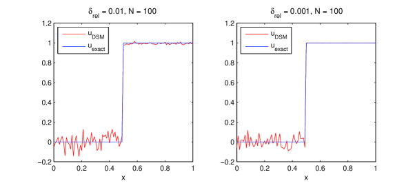
Figure 1. Plots of solutions obtained by the iterative scheme when $N=100$, $\delta_{rel}=0.01$ (left) and $\delta_{rel}=0.001$ (right).

Figure 2 plots the numerical results when the noise levels are $\delta_{rel}=0.01$ and $\delta_{rel}=0.001$. In this experiment we choose the noise function by the formula $f_{noise}(x)=\sin(3\pi x),x\in[0,1]$.

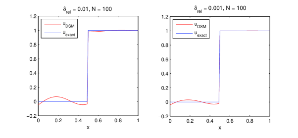
Figure 2. Plots of solutions obtained by the iterative scheme when $N=100$, $\delta_{rel}=0.01$ (left) and $\delta_{rel}=0.001$ (right).

In computations the functions $u,f$ and $f_{\delta}$ are vectors in $\mathbb{R}^{N}$ where $N$ is the number of nodal points. The norm used in computations is the Euclidean length or $L^{2}$ norm of $\mathbb{R}^{N}$.

We have also carried out numerical experiments with $a_{n}=\frac{10}{(5+n)^{0.99}}$. For this choice of $a_{n}$ the convergence of $u_{n_{\delta}}$ to the unique solution of the problem is guaranteed by Theorem 3.1–3.5. However, the numerical experiment showed that using this choice of $a_{n}$ does not bring any improvement in accuracy while requiring more time for computation. Experiments also showed that for this problem it is better to use $a_{n}=\frac{a(0)}{(5+n)^{0.99}}$ with $a(0)\in[0.1,1]$.

From the numerical results we conclude that the proposed stopping rule yields good results in this problem.

References

- [1] A. Bakushinskii and A. Goncharskii, Ill-Posed Problems: Theory and Applications, Dordrecht, Kluwer, 1994.
- [2] K. Deimling, Nonlinear functional analysis, Springer-Verlag, Berlin, 1985.
- [3] N. S. Hoang and A. G. Ramm, An iterative scheme for solving nonlinear equations with monotone operators. BIT, 48, N4, (2008), 725-741.
- [4] N. S. Hoang and A. G. Ramm, Dynamical Systems Gradient method for solving nonlinear equations with monotone operators, Acta Appl. Math., 106, (2009) , 473-499.
- [5] N. S. Hoang and A. G. Ramm, A new version of the Dynamical systems method (DSM) for solving nonlinear quations with monotone operators, Diff. Eq. Appl., 1, N1, (2009), 1-25.
- [6] Hoang, N.S. and Ramm, A. G., Dynamical systems method for solving nonlinear equations with monotone operators, Math. Comp., 79, (2010), 239-258.
- [7] V. Ivanov, V. Tanana and V. Vasin, Theory of ill-posed problems, VSP, Utrecht, 2002.
- [8] V. A. Morozov, Methods of solving incorrectly posed problems, Springer-Verlag, New York, 1984.
- [9] A. G. Ramm, Dynamical systems method for solving operator equations, Elsevier, Amsterdam, 2007.
- [10] A. G. Ramm, Global convergence for ill-posed equations with monotone operators: the dynamical systems method, J. Phys A, 36, (2003), L249-L254.
- [11] A. G. Ramm, Dynamical systems method for solving nonlinear operator equations, International Jour. of Applied Math. Sci., 1, N1, (2004), 97-110.
- [12] A. G. Ramm, Dynamical systems method (DSM) and nonlinear problems, in the book: Spectral Theory and Nonlinear Analysis, World Scientific Publishers, Singapore, 2005, 201-228. (ed J. Lopez-Gomez).
- [13] A. G. Ramm, Dynamical systems method (DSM) for unbounded operators, Proc. Amer. Math. Soc., 134, N4, (2006), 1059-1063.
- [14] U. Tautenhahn, On the method of Lavrentiev regularization for nonlinear ill-posed problems, Inverse Problems 18 (2002) 191 207.
- [15] V. V. Vasin and A. L. Ageev, Ill-Posed Problems with a Priori Information, Utrecht, VSP, 1995.