Radio galaxy feedback in X–ray selected groups from COSMOS: the effect on the ICM

Abstract

We quantify the importance of the mechanical energy released by radio-galaxies inside galaxy groups. We use scaling relations to estimate the mechanical energy released by 16 radio-AGN located inside X-ray detected galaxy groups in the COSMOS field. By comparing this energy output to the host groups’ gravitational binding energy, we find that radio galaxies produce sufficient energy to unbind a significant fraction of the intra-group medium. This unbinding effect is negligible in massive galaxy clusters with deeper potential wells. Our results correctly reproduce the breaking of self-similarity observed in the scaling relation between entropy and temperature for galaxy groups.

1. Introduction

Galaxy groups are important laboratories in which to investigate the importance of non–gravitational processes in structure formation. These processes are potentially more important in galaxy groups than in massive clusters because of their lower gravitational binding energy. This is suggested by the significant deviation of the observed X–ray luminosity and entropy versus temperature ($L_{X}$–T and $S$–T) scaling relations in groups compared to the relation expected in a purely gravitational scenario (see also Pratt & Arnaud 2003; Markevitch 1998; Arnaud & Evrard 1999; Ponman et al. 2003; Sun et al. 2009; Pratt et al. 2009). Radiative cooling can be invoked to explain this deviation, but then the predicted fraction of stars in clusters of a given mass is incorrect (Voit, 2005; Balogh et al., 2008). To simultaneously explain the properties of the intra–cluster/group medium (ICM) and account for the observed properties of galaxies, it is necessary to take into account a major contribution to the cluster/group energetics from non–gravitational heating.

The two main sources of non–gravitational heating are star–formation and active galactic nuclei (AGN). Cosmological simulations (e.g. Kay 2004; Bower et al. 2006; Sijacki & Springel 2006) show that both processes are required to reproduce the properties of the ICM. In particular, recent simulations by Bower et al. (2008) successfully reproduce both the galaxy and ICM properties (see Short & Thomas 2009) when they include a ”radio–mode” AGN feedback phase: in this phase the movement of bubbles inflated by the AGN jets transfers energy into the gas within the cluster (mechanical heating). The observable objects providing this type of feedback inside groups and clusters would be radio galaxies (Croton et al., 2006). The main difference between the Bower et al. (2008) model and others, including radio–mode AGN, (Bower et al. 2006; Sijacki & Springel 2006; Puchwein et al. 2008;) is that it allows the radio mode feedback to expel gas from the X-ray emitting regions of the system.

The importance of such AGN-feedback in groups could explain the observational result by Lin et al. (2003), McCarthy et al. (2007) and Giodini et al. (2009), that the total baryon fraction in groups is lower than the cosmic value estimated from cosmic microwave background (CMB) observations (see Giodini et al. 2009 for more details). The discrepancy decreases in systems of higher total mass, such that it is $<$1$\sigma$ for massive clusters.

In this Paper we propose a simple, direct method to test the hypothesis that radio galaxies in groups can indeed inject enough mechanical energy to unbind the intra–cluster gas. The Paper is structured as follows. In Section 2 we select a sample of 16 groups from the COSMOS 2 deg² survey discussed in Giodini et al. (2009), each hosting a radio galaxy within the virial radius (Schinnerer et al. 2007; Smolčić et al. 2008), plus a control sample of massive clusters from Bîrzan et al. (2004). In Sections 3 and 5 we then compare the groups’ binding energy to the mechanical energy output by the radio sources, derived from their total radio luminosity through scaling relations. Applying this method, we show that the mechanical removal of gas from the group region is indeed energetically feasible for systems below $\sim$3$\times$10¹⁴M_⊙. In Section 6 we discuss how this scenario compares to the deviation in the scaling relation between entropy and temperature at the groups scale.

We adopt a $\Lambda$CDM cosmology with $h$=0.72, $\Omega_{m}$=0.25, $\Omega_{\Lambda}$=0.75.

2. The samples

2.1. Radio galaxies in X–ray detected groups

We use the catalog of 91 X–ray selected groups from the COSMOS survey (Scoville et al. 2007a; Finoguenov et al. in preparation), selected as described in Giodini et al. (2009). Extended source detection was performed using a multiscale wavelet reconstruction of a mosaic of XMM and Chandra data. For each group, member galaxies are identified within R₅₀₀ of the group center, utilizing the high quality photometric redshifts available ($\sigma(\Delta z)/(1+z)$=0.02 at i${}_{AB}<$25, Ilbert et al. 2009).

We use a sub-sample of the VLA–COSMOS catalog (Schinnerer et al. 2007; Smolčić et al. 2008) to identify radio galaxies lying inside the X–ray selected groups. Of the $60$ radio galaxies identified within the VLA-COSMOS Large Project (Schinnerer et al. 2007; 1.49 GHz), about 80% have been associated with a secure optical counterpart (Smolčić et al., 2008) with $i_{\mathrm{AB}}\leq 26$, and accurate photometry (thus also with accurate photometric redshifts; Ilbert et al. 2009; Salvato et al. 2009).

We have cross-correlated this sample of radio galaxies with the X-ray selected galaxy groups in 3D space using a search radius of $1\times R_{200}$ (Finoguenov et al. in preparation) around the groups’ centers and within 0.02$\times$(1+z) from the group’s redshift. This resulted in a sample of 16 systems matched in position and redshift. In Appendix A we show the contours of the radio 20 cm and X–ray emission superimposed to the SUBARU $zp$ band image for each of the groups. In 9 out of 16 cases the radio galaxy is located in the core of the group (defined as $R<$0.15$R_{200}$). The 20 cm radio luminosity densities of these galaxies range from $\sim 5.5\times 10^{22}-4.8\times 10^{25}$ W Hz^-1, with a median luminosity of $8.9\times 10^{24}$ W Hz^-1($\nu\,F_{\nu}\sim 7.3\times 10^{38}-6.4\times 10^{41}$ erg s^-1, with a median luminosity of $1.18\times 10^{41}$ erg s^-1) . This median luminosity is at the high end of the radio luminosity distribution of the full radio AGN sample (c.f. Fig. 17 in Smolčić et al. 2008, and Fig. 5 in Smolčić et al. 2009), consistent with previous findings that powerful radio galaxies inhabit group-scale environments (e.g. Baum et al. 1992). The redshift distribution of the 16 groups is fairly uniform between 0.1 and 1, with the exception of 6 sources concentrated at z$\sim$0.3 (where a large structure extends throughout the whole COSMOS field). The groups have X–ray luminosities ranging from 1$\times$10⁴² to 8.7$\times$10⁴³ erg s^-1 and span a mass range of 2$\times$10${}^{13}<$M${}_{200}<$2$\times$10¹⁴M_⊙ with a median mass of 7.14$\times$10¹³M_⊙.

2.2. The comparison sample of massive clusters

The COSMOS X–ray sample is mostly composed of groups. We complement it with 12 well known radio galaxies inside massive clusters, extracted from the sample of Bîrzan et al. (2004). We use those clusters from the Birzan’s sample which overlap with the HIFLUGCS survey (Reiprich & Boehringer, 2002) so that we can use the X–ray parameters determined from the HIFLUGCS clusters. In addition we require that the radio source within those clusters is associated with a secure NIR counterpart in the 2MASS catalogue (Skrutskie et al., 2006). These requirements eliminate 4 of the clusters in the original Birzan et al. sample. Each of these clusters contain X–ray cavities associated with radio bubbles likely connected with AGN activity of the central galaxy. The radio galaxies have been identified within the NRAO VLA Sky Survey (NVSS) at 1.49 GHz (Condon et al., 1998), except in the case of the Centaurus Cluster where data come from the 1.41 GHz Parkes Radio Sources Catalogue (Wright & Otrupcek, 1990). The 20 cm radio luminosities of the radio galaxies range between 2$\times$10³⁹ and 2 $\times 10^{43}$ erg s^-1, with a median luminosity of 1.4$\times 10^{42}$ erg s^-1, more than 10 times higher than the median radio luminosity of the radio galaxies in the COSMOS sample.
The X–ray parameters for these clusters are provided by the X–ray analysis in the HIFLUGCS survey, and converted for the standard cosmology used in this paper. The sample consists of very local clusters, ranging in total mass between 1$\times$10${}^{14}<$M${}_{200}<$1.2$\times$10¹⁵M_⊙ with a median mass of 4.25$\times$10¹⁴M_⊙, almost 10 times higher than the median total mass of the systems in the COSMOS sample

3. Analysis of COSMOS group sample

3.1. Mechanical energy input by radio galaxies in groups

We estimate the mechanical energy input by a radio galaxy into the ICM over the group lifetime from the mechanical luminosity of the radio source multiplied by the fraction of time a massive galaxy spends in the radio-AGN phase. The mechanical luminosity for the radio galaxies in our sample is estimated from the scaling relation presented in Bîrzan et al. (2008). These authors studied a sample of galaxy clusters showing signatures of cavities and bubbles in the X-ray surface brightness 2D distribution, with a powerful radio source as a central galaxy. The cavity power of the radio source, estimated from the $p{\mathrm{d}}V$ work of the jet/lobe on the surrounding ICM, is found to be correlated (albeit with a large scatter) with the monochromatic radio power at 1.49 GHz of the central galaxies ($P_{1.49\,GHz}$) as

$$P_{cav}\propto P_{1.49\,GHz}^{0.35\pm 0.07}$$ (1)

(see Eq. 16 in Bîrzan et al. 2008). $P_{1.49\,GHz}$ is computed from the radio–emission of the entire source. This estimate is a lower limit to the mechanical luminosity of the AGN outbursts, since it does not take into account the energy dissipated (e.g. in shocks). $P_{\mathrm{cav}}$ is related to the $p{\mathrm{d}}V$ work through

$$P_{cav}=\frac{4PV}{\tau}$$ (2)

(Churazov et al. 2002; Bîrzan et al. 2008), where $\tau$ is the duration of each single AGN outburst and 4 is the factor used for relativistic plasma. Smolčić et al. (2009) investigated the fraction of radio AGN as a function of cosmic time and stellar mass of the galaxy. This fraction can be related, through a probability argument detailed in Smolčić et al. (2009), with the time a galaxy of a given stellar mass and at a given redshift spends as a radio galaxy ($\tau_{\mathrm{radio}}$). Using this result we can estimate the average duration of radio sources as a function of redshift and stellar mass of the host galaxy (see Fig. 12 in Smolčić et al. 2009). This gives a plausible time-scale during which the radio AGN can have injected mechanical energy into its environment. For the 16 COSMOS X–ray selected groups, $\tau_{radio}$ ranges between 0.003 and 4.18 Gyr, with a median value of 3.1 Gyr. The mechanical energy contribution can then be estimated as

$$E_{\mathrm{mech}}=P_{\mathrm{cav}}\times\tau_{\mathrm{radio}}.$$ (3)

The values of E_mech for our sources are shown in Table 1 and span a range between $\sim$2$\times$10⁵⁷–3$\times$10⁶¹ erg h${}_{72}^{-2}$. The uncertainties in the radio mechanical energy input are dominated by the scatter in the scaling relation used to convert the monochromatic power into mechanical luminosity, which amounts to 0.85 dex, and by the uncertainties on $\tau_{\mathrm{radio}}$. We use $\tau_{\mathrm{radio}}$ as derived from an average estimate over a sample of radio galaxies in the COSMOS field as a whole, irrespective of their environment. One might expect the density of the environment surrounding the jets to have a significant impact on the jet lifetime. However, the fraction of radio galaxies that resides within the COSMOS groups is comparable with the fraction of red massive galaxies within groups in the control sample used in Smolčić et al. (2009) (respectively 18$\%$ and 16$\%$ within $R_{200}$); this assures that the statistical argument used to compute the time–scales holds also in this case. Furthermore we can estimate an average time–scale based on only extended radio galaxies in the whole COSMOS group sample as follows. Of the 141 COSMOS groups at $z<1$ and with L${}_{X}>10^{42}$ erg s^-1, 32 contain a multi-component radio galaxy. Therefore the average duration of the radio galaxy activity during this time interval is $(32/141)\times(t(z=1)-t(z=0))$. This is $\sim 1.7$ Gyr, a time-scale comparable with the average life-time estimated with the method by Smolčić et al. (2009) ($\sim$1.6 Gyr.

Table 1 For each of the 16 COSMOS groups, the columns indicate 1) X–ray catalogue ID number 2) R.A. 3) Dec. 4) redshift 5) Power at 1.4 GHz 6) Mechanical Power 7)Binding energy $\pm$ 1$\sigma$ confidence limit 8) $E_{mech}$ $\pm$ 1$\sigma$ confidence limit 9) $\tau_{\mathrm{radio}}$ 10) distance from the center

XID	R.A.	DEC.	$z$	P${}_{1.49\,GHz}$	Pcav	$E_{\mathrm{binding}}$	$E_{\mathrm{mech}}$	$\tau_{\mathrm{radio}}$	$R/R_{200}$
	[J2000]	[J2000]		[$10^{24}$ W/Hz]	[$10^{36}$ W]	[1060erg]	[$10^{60}$ erg]	[Gyr]
107	149.60965	2.14799	0.28	1.11	7.353	5.916${}_{1.937}^{2.342}$	0.514${}_{0.441}^{3.087}$	0.221	0.3783
262	149.60007	2.82118	0.34	19.0	19.85	127.9${}_{26.49}^{38.80}$	24.15${}_{20.70}^{144.9}$	3.858	0.0011
253	149.75626	2.79472	0.49	6.71	13.78	40.16${}_{9.721}^{12.26}$	10.14${}_{8.693}^{60.85}$	2.332	0.0042
246	149.76132	2.92909	0.34	0.90	6.828	289.8${}_{67.46}^{76.73}$	7.003${}_{6.003}^{42.02}$	3.252	0.6181
311	149.93796	2.60627	0.34	6.38	13.54	17.27${}_{3.907}^{4.792}$	0.183${}_{0.157}^{1.101}$	0.042	0.2195
264	149.99847	2.76914	0.16	0.32	4.775	6.940${}_{2.247}^{3.179}$	0.004${}_{0.003}^{0.027}$	0.003	0.0007
281	150.08617	2.53141	0.88	8.90	15.21	84.94${}_{22.45}^{27.05}$	1.241${}_{1.064}^{7.450}$	0.258	0.8614
191	150.11434	2.35651	0.22	1.71	8.554	8.380${}_{2.150}^{2.959}$	6.122${}_{5.248}^{36.73}$	2.269	0.0757
237	150.11774	2.68425	0.34	27.7	22.65	105.1${}_{23.49}^{31.65}$	19.56${}_{16.77}^{117.4}$	2.738	0.0027
29	150.17996	1.76887	0.34	30.0	23.29	58.49${}_{12.77}^{16.80}$	31.63${}_{27.11}^{189.8}$	4.306	0.0016
64	150.19829	1.98628	0.43	12.4	17.11	21.10${}_{4.941}^{7.358}$	18.06${}_{15.48}^{108.4}$	3.348	0.0030
35	150.20661	1.82327	0.52	10.2	16.00	30.87${}_{8.342}^{11.07}$	15.32${}_{13.13}^{91.95}$	3.037	0.0008
6	150.28821	1.55571	0.36	1.13	7.401	77.91${}_{17.35}^{20.23}$	0.070${}_{0.060}^{0.425}$	0.030	0.2279
149	150.41566	2.43020	0.12	0.05	2.564	50.31${}_{10.32}^{14.98}$	0.002${}_{0.002}^{0.014}$	0.003	0.1957
40	150.41386	1.84759	0.96	48.5	27.54	108.1${}_{24.40}^{34.85}$	1.786${}_{1.530}^{10.71}$	0.205	0.4888
120	150.50502	2.22506	0.83	16.4	18.88	425.0${}_{90.06}^{112.5}$	24.92${}_{21.36}^{149.5}$	4.185	0.0267

3.2. Binding energy of the intra–group medium

We consider the shape of the dark matter halos to be characterized by NFW (Navarro et al., 1996) radial profiles

$$\rho(x)=\frac{\rho_{\mathrm{crit}}\,\delta_{c}}{x\,(x+1)^{2}}$$ (4)

where $x=r/r_{s}$, $r_{s}$ is the characteristic radius, and $\rho_{c}$ is the critical density of closure of the universe. $\delta_{c}$ is defined as

$$\delta_{c}=\frac{200\,c^{3}}{3\,\ln(1+c)-c/(1+c)}$$ (5)

and $c$ is the concentration of the halo. The scale radius and the concentration are linked by the relation $r_{s}=R_{500}/c_{500}$, where $c_{500}$ is the dark matter concentration inside $R_{500}$. We estimate the binding energy out to $R_{500}$ because the kinetic energy of the infall velocity field along filaments becomes important beyond this radius (Evrard et al., 1996) and our simple model may not then be applicable. Furthermore, we can evaluate reliable gas masses from the X–ray observations only within $R_{500}$. For simplicity, we assume that the gas follows the same distribution as the dark matter. We define as binding energy the total potential energy needed to push the ICM gas inside $R_{500}$ beyond $R_{200}$. The binding energy is computed as

$$E_{\mathrm{binding}} = \int^{M_{g,500}}_{0}\left[\phi(r)-\phi(R_{200})\right]\,dM_{g}$$ (6)

$$= 4\,\pi\int^{R_{500}}_{0}\phi(r)\,\rho_{g}(r)\,r^{2}\,dr$$

We neglect the additive constant given by the term $\phi(R_{200})$, as it is small with respect to the other terms of the equation. We use the definition of gas mass within R₅₀₀ as

$$M_{g}=M_{g}(R_{500})=4\,\pi\,\int^{R_{500}}_{0}\rho_{g}(r)\,r^{2}\,dr.$$ (7)

The potential of a spherical NFW model is (Hayashi et al., 2007)

$$\phi(r)=A\times\frac{ln(1+x)}{x}$$ (8)

where A is

$$A=-\frac{G\,M_{200}}{r_{s}\,(ln(1+c)-c/(1+c))}$$ (9)

Thus, substituting the terms into Equation 6, we compute the binding energy of the ICM gas in a NFW dark matter halo as follows:

$$E_{\mathrm{binding}}=f_{gas}4\,\pi\,\rho_{crit}\,\delta_{c}\,A\,r_{s}^{3}\int^{c_{500}}_{0}\frac{ln(1+x)}{(1+x)^{2}}\,dx$$ (10)

where $f_{\mathrm{gas}}$ is the gas fraction. The concentration parameter for the COSMOS groups has been computed from the mass-dependent relation of Macciò et al. (2007). The errors bars on the binding energy are estimated using a Monte Carlo method to numerically propagate the errors on $M_{200}$ and $R_{200}$, the scatter in the $c$–$M_{200}$ and in the $f_{\mathrm{gas}}$–$M_{500}$ relation.
We cannot estimate the gas masses from most of the existing X-ray observations of the COSMOS X–ray selected groups because of insufficient signal-to-noise. We therefore estimate the gas fraction in the groups from the mean trend of the gas mass fraction as a function of M₅₀₀. This trend was established from an independent compilation of high quality observations of local (z$<$0.2) groups and clusters in the same mass range as the sample under consideration here (Pratt et al., 2009). The observed relation ($f_{\mathrm{gas}}\propto$M${}_{500}^{0.21}$) suggests that lower mass systems have proportionally less gas than high mass systems.

4. Analysis of galaxy cluster sample

4.1. Mechanical energy input by radio galaxies in massive clusters

In order to compare the energy input from radio galaxies in groups and clusters, we include in our analysis a sample of well known radio galaxies in massive clusters, extracted from the sample of (Bîrzan et al. 2004; see Section 2.2). We use their tabulated value of $p\mathrm{d}V$ to compute the mechanical energy input over the average time the galaxy has spent as a radio galaxy. Birzan et al. provide a value for the energy input for both filled and radio ghost cavities. In order to obtain a measure of the average input, we sum the $pdV$ for all the cavities in a cluster and multiply it by the number of events (i.e. how often the radio jet was turned on). The latter is given by the ratio between $\tau_{radio}$ and the duration of a single radio event (assuming that all the active AGN phases have the same duration).

We choose the oldest cavity’s age as an indication of the duration of the radio event. Bîrzan et al. (2004) calculate the age of each cavity in three ways: 1. the time required for the cavity to rise at the sound velocity; 2. the time required for the bubble to rise buoyantly at the terminal velocity; 3. the time required to refill the displaced volume. We adopt the average of the three age estimates; this is generally similar to the age computed for a buoyantly rising bubble. We take the error on the cavity’s age to be the difference between the shortest and longest life–time estimated via the three different methods.

As $\tau_{\mathrm{radio}}$ for our sample is derived following Smolčić et al. (2009), it depends on the redshift and the stellar mass of the radio galaxy. We computed the stellar masses for the central radio galaxy in the massive cluster sample using the K–band photometry provided by the 2MASS survey (Skrutskie et al., 2006). This method is robust, since radio galaxies contain mostly type 2 (obscured) AGN, whose emission does not significantly contaminate the optical–NIR part of the galaxy spectrum. We assume a M/L_K ratio for a stellar population with an age of $\sim$10 Gyr (corresponding to the age of the stars in a galaxy at z$\sim$0), obtained by Drory et al. (2004) (M/L_K=1.4 with a Salpeter IMF). The quoted error on the M/L_K in Drory et al. (2004) is 25–30$\%$: a change in stellar mass of this magnitude does not affect significantly the time–scales we estimate. The stellar masses are then converted to a Chabrier IMF by subtracting an offset of 0.2 dex.

4.2. Binding energy of the intra–cluster medium

We compute the binding energy for the Birzan et al. clusters in the same way as for the COSMOS groups, using the value of M₂₀₀ and R₂₀₀ provided by the X–ray analysis in the HIFLUGCS survey (Reiprich $\&$ Boehringer 2002). We assume a constant concentration parameter of 5. Errors on $E_{\mathrm{binding}}$ are propagated numerically via a Monte Carlo method, in the same way as the COSMOS groups (see Section 3.2). As well as computing the binding energy of clusters individually, we also test the cluster result using the scaling relations adopted for the COSMOS groups, both for computing M₂₀₀ (Leauthaud et al., 2010) and for estimating their mechanical energy output (Bîrzan et al., 2008). The change in our calculations does not qualitatively affect our results. The values of $E_{\mathrm{binding}}$ change by less than a factor 2 on average, while values of $E_{\mathrm{mech}}$ are perturbed randomly within the error bars.

5. Results

5.1. The balance of radio–input and binding energy

Figure 1 shows the binding energy of the gas versus the energy output from radio galaxies. In the group regime, the two energies span a comparable range of values (10⁵⁸–10⁶¹ ergs), while for clusters the binding energy exceeds the total mechanical output of radio–galaxies by a factor approximately of $\sim$10²–10³. In particular, for seven groups the two energies are consistent at 1$\sigma$ level, and for all other groups except two the equality holds at 3$\sigma$, meaning that radio–galaxies potentially provide sufficient energy to unbind the gas in a large fraction of these groups. It is interesting to note that, in all the groups with E${}_{mech}\sim$E_binding, the radio galaxy lies within 0.15$\times$R₂₀₀ from the center of the group. This suggests that a radio galaxy in a group is most likely to input sufficient energy into the ICM to unbind a part of the gas if it lies at the core of the group. Moreover, radio sources outside the group core reside in lower density environments, and our calculations of those binding energies may be overestimates. The different energy balance in groups and clusters demonstrates the importance of AGN heating in groups, and shows that the mechanical removal of gas from groups is energetically possible. This has important consequences for the understanding of the baryonic budget in these systems (see Giodini et al. 2009).

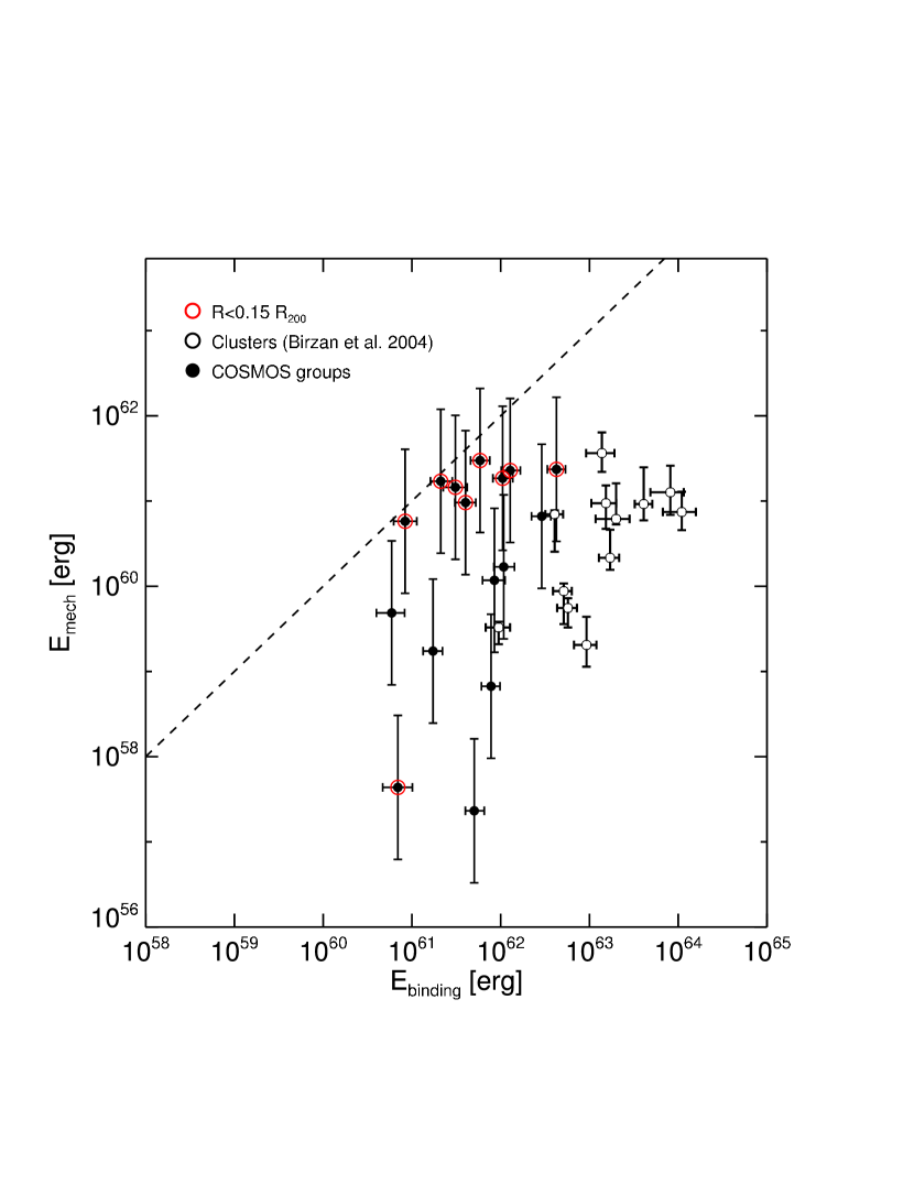
Figure 1.— Binding energy of the cluster/group gas versus the output mechanical energy from radio–galaxies. Solid points show the 16 X–ray selected groups in the COSMOS field that host a radio galaxy within their virial radius. Large concentric circles indicate groups that host a radio galaxy within the core (R$\leq 0.15\times R_{200}$). Open points show the sample of massive local clusters drawn from Bîrzan et al. 2004. The dashed line shows equality. The binding energy in clusters exceeds the total mechanical output by a factor of $\sim$10²–10³. In all cases except one where a radio galaxy lies in the centre of a group, the mechanical energy output from the radio galaxy is of the same order as the binding energy for the COSMOS groups analyzed here.

5.2. Can radio galaxies offset radiative cooling in galaxy groups?

We now compare the mechanical energy input by radio–galaxies with the energy required to offset the cooling in the group center ($E_{\mathrm{cool}}$). As detailed in Fabian et al. (1994), Peterson et al. (2003) and McNamara & Nulsen (2007), the cooling time in cluster/group centers can be lower than the Hubble time, implying that large reservoirs of cold gas could accumulate in these regions. However, evidence that the gas does not cool below approximately one third of the virial temperature (Kaastra et al., 2004) indicates the presence of a heat source providing enough energy to offset the cooling. Several studies (e.g. Peterson et al. 2003, Peterson & Fabian 2006, McNamara & Nulsen 2007) suggest AGN feedback as a viable heating source. To test this hypothesis, we check whether the cooling energy is lower than the mechanical energy of the rising bubbles. We estimate $E_{\mathrm{cool}}$, assuming that the time during which the gas has been cooling is equal to the lifetime of the group, which we assume to be 5 Gyr (Voigt & Fabian, 2004). The cooling energy can then be estimated as:

$$E_{\mathrm{cool}}=L_{\mathrm{cool}}\times t_{v}=f_{\mathrm{cool}}\,L_{\mathrm{bol}}\times t_{v}$$ (11)

where $t_{v}$ is the lifetime of the group, and $f_{\mathrm{cool}}$ is the fraction of bolometric luminosity assumed to be emitted inside the cooling radius (where the cooling time of the gas is lower than the Hubble time). In general this contribution is found to be $\gtrsim$10$\%$ of the total cluster X–ray luminosity (McNamara & Nulsen, 2007). Also, the scatter in the L_X–T scaling relation due to the contribution of cool core clusters can be up to a factor of 2 (Chen et al. 2007; Pratt et al. 2009). Given these considerations, we assume that $25\%$ of the total bolometric X–ray luminosity is emitted inside the cooling radius (Peres et al., 1998). Since the relative contribution of the cool core to the total X–ray luminosity is higher in groups than in massive clusters, this value is a good estimate of the average contribution of the cooling core to the total luminosity of a group.
In Figure 2 we compare $E_{\mathrm{mech}}$ and $E_{\mathrm{cool}}$ in our groups. The mechanical energy injected by all but one of the core radio–galaxies is higher than the radiative losses, and exceeds $E_{\mathrm{cool}}$ by an order of magnitude in several cases. We can thus conclude that radiative losses do not greatly affect the net energy output of radio–galaxies in the cores of groups. On the other hand, the mechanical output by non-central radio galaxies is typically of the same order as $E_{\mathrm{cool}}$. Moreover, these sources reside mostly outside the cooling radius ($\sim$0.15 R₂₀₀), where the cooling time is higher than the Hubble time. In this location, the gas does not lose as much energy through radiative cooling as in the core of the group, so these galaxies do not provide the required feedback at the right location.

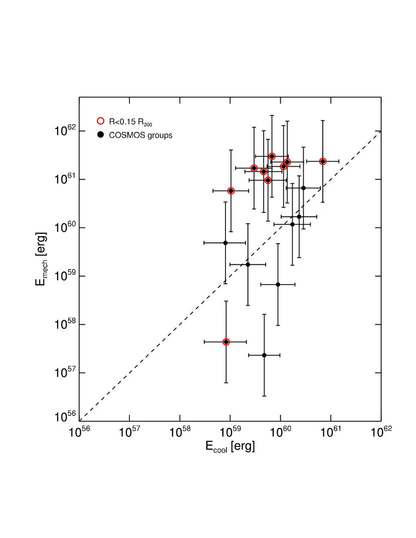
Figure 2.— The output mechanical energy from radio–galaxies (E_mech) versus energy radiated inside the cooling radius (E_cool; i.e. energy required to offset the cooling in the group center) for 16 X–ray selected groups from the COSMOS survey . The dashed line shows the equality line. Red circles mark the radio–galaxies inside $0.15\times R_{200}$. Uncertainties on $E_{\mathrm{cool}}$ are computed allowing an error of a factor 2 on $f_{\mathrm{cool}}$.

5.3. Impact of systematic effects

The above calculations rest on several assumptions and should be regarded as rough estimates. One critical simplification is the calculation of the lifetime of a radio–galaxy: the statistical argument used in Smolčić et al. (2009) relies on knowledge about the parent population that hosts the radio–galaxies. In the absence of evidence to the contrary, we assume that there is no significant difference between the radio–galaxy elliptical hosts in groups and in low density environments (Feretti & Giovannini, 2007). We note that even if $\tau_{\mathrm{radio}}$ were incorrect by a factor of 4, the mechanical output in clusters would still be significantly lower than the binding energy, but would remain consistent with the binding energy for many of the groups (see Figure 1).

Other biases may arise from the scaling relation of Birzan et al., which we use to compute the mechanical energy: the large scatter in the P${}_{1.49\,GHz}$–P_cav relationship (0.85 dex) means that care must be taken when using the inferred value as the mean mechanical energy, since most of our calculations rest on the assumption that over the cluster/group lifetime each burst has on average the same power. Indeed, Nipoti & Binney (2005) suggested that the distribution of the outbursts over the cluster/group lifetime is log–normal rather than gaussian; therefore in any system there would be a good chance of observing smaller than average jet powers. Instead, much of the power would be generated by rare, more powerful outburst, such as that observed in MS 0735+7421 by Gitti et al. (2007). These arguments rest on the assumption that the observed scatter in P${}_{1.49\,GHz}$–P_cav in the observed ensemble of clusters is a good description of the time variability of the AGN power in individual objects. In general the ensemble scatter is an upper limit to the scatter in the time variability. If we assume this scatter to represent also for the time variability, we are statistically underestimating the mechanical energy output over the group lifetime by a factor that we compute as follows. The scatter in the Birzan et al. relationship (0.85 dex) corresponds to a probability $\gtrsim$80$\%$ of observing a value smaller than the mean from a single observation (cf. Nipoti & Binney 2005). Thus, if we assume that the observed value of P${}_{1.49\,GHz}$ scatters around the median of the distribution, the ratio between the median and the mean for a lognormal distribution (which depends only on the scatter $\sigma$) tells us the scaling factor for the ’true’ mean mechanical energy:

$$\frac{mean}{median}=\frac{e^{\sigma^{2}}}{2}=6.8.$$ (12)

Therefore the typical observed mechanical power may be underestimated by a factor $\leq$7 with respect to the mean. This value, though not negligible, goes in the direction of further increasing the mechanical output, confirming the effect we found.
Furthermore, if the bubble were over–pressured when compared to the surrounding ICM (Heinz et al., 1998), the expanding bubble would carry a shock and the mechanical power may be underestimated, as well as reported by Bîrzan et al. (2004). This effect would also boost the mechanical energy to higher values, further strengthening our results.

We have also used preliminary results from VLA 324 MHz data (Smolcic et al. in preparation) to double-check our estimates of the mechanical energy output from radio–galaxies. Only 12 of the 16 radio–galaxies are detected in the 324 MHz band and, in all these cases, $E_{\mathrm{mech}}$ computed using these data (using Eq.15 in Bîrzan et al. 2008) is consistent within the error bars with the value computed at 1.49 GHz. As a further check, the total radio luminosity can be computed with higher precision from break frequencies for 7 of the 16 sources, using the the Myers & Spangler (1985) approximation. The value of $E_{\mathrm{mech}}$ obtained with this improved method is consistent within the error bars with that obtained using monochromatic data.

6. Discussion: the entropy in X–ray groups

The injection of energy by radio galaxy activity into the ICM modifies the thermodynamical state of the gas, raising the entropy ($S$) by a significant amount compared to that generated by gravitational collapse. We define the entropy as

$$S\propto\frac{kT}{n_{e}^{\frac{2}{3}}}$$ (13)

where T is the gas temperature in keV and n_e is the gas electron density (Voit, 2005). An excess entropy of 50–100 keV cm^-2 is indeed observed at the group regime, causing a deviation from the $S$–T relation (Ponman et al., 2003). The excess entropy is measured in the central regions (at 0.1 R₂₀₀). In the following we make an order of magnitude calculation of the excess entropy generated by the energy injected, then compare it with that observed in groups and predicted from the theory. We recompute the expected S–T relation taking into account this excess energy, and compare it with the observational constraints of Ponman et al. (2003).

The change in entropy caused by injection of energy under constant pressure is

$$\Delta S=\frac{2}{5}\frac{\Delta E}{n_{e}}\frac{\gamma_{T}^{5/3}-1}{\gamma_{T}-1}$$ (14)

(Lloyd-Davies et al., 2000), where $\Delta E$ is the injected energy per particle, $\gamma_{T}$ is the ratio between the initial and final temperature (a value between 1.1 and 2.0, Lloyd-Davies et al. 2000), and $n_{e}$ is the initial electron density ($n_{e}$=10^-2 assuming the energy is deposited in the cluster core, e.g. Sanderson & Ponman 2003). We compute $\Delta E$ from the mechanical energy input of radio galaxies as follows:

$$\Delta E=E_{\mathrm{mech}}\times\frac{m_{p}\mu}{M_{gas}}$$ (15)

with $M_{\mathrm{gas}}=f_{\mathrm{gas}}\,M_{200}$, where $f_{\mathrm{gas}}$ is estimated from the relation between gas fraction and total mass in Pratt et al. (2009). This calculation does not depend on the details of the energy injection process. We obtain values of excess entropy between 10 and 60 keV cm^-2. This is a rough calculation but predicts values similar to those in Voit & Donahue (2005). These authors show that an additional energy input episodic on $10^{8}$ yrs timescale is needed to explain the excess entropy found observationally in the core of clusters (Ponman et al., 2003; Donahue et al., 2005). The additional energy produces an entropy pedestal: Voit (2005) calculates 10 keV cm^-2 to be the minimum entropy boost needed to explain observations, and he predicts it to be larger for groups.

The mechanical energy injected by radio galaxies into the 16 COSMOS X-ray selected groups is roughly independent on the group mass (see Figure 1). This is not unexpected, since the black–hole masses (which are a zeroth order indicator of the mechanical energy output; Merloni & Heinz 2007) range only between 10⁸–10⁹ M_⊙ in radio galaxies (see Figure 7 in Smolčić et al. 2009). At the cluster regime may not be true that the mechanical energy is independent on cluster mass. Indeed Chen et al. (2007) infer, from the strength of clusters’ cooling cores, that a mechanical input higher than anything observed in groups is necessary to balance the cooling of the gas in the strong cool core clusters. However, it has been shown by the same authors that much ($\sim$90%) of that energy input would be radiated away to balance the cooling, and therefore would not participate to the mechanical removal of the gas.

From these considerations, we can predict how the scaling relation between entropy and temperature is affected by the injection of a constant excess energy by radio galaxies. As shown in Finoguenov et al. (2008), the energy deposition into the ICM ($\Delta E$) is proportional to the change in entropy $\frac{\Delta S}{S}$ for a given typical n_e. We use n_e=10^-2 as the typical value of the density within 0.1 R₂₀₀, where the majority of the energy is deposited ( deposition radius;Sanderson & Ponman 2003). Using the scaling of $M_{\mathrm{gas}}\propto$T² and $E_{\mathrm{mech}}=\,const$, then

$$\frac{\Delta S}{S}\propto\frac{E_{\mathrm{mech}}}{M_{gas}}\propto\frac{C}{T^{2}}.$$ (16)

where $C$ is a constant and M_gas is the mass of the gas within the deposition radius. We can then infer the functional dependence of $S$ on the virial temperature of the ICM as

$$S=S_{0}+\Delta S=S_{0}\times(1+\frac{\Delta S}{S_{0}})\propto(T_{0}+\frac{C}{T_{0}}),$$ (17)

where $S_{0}$ and T₀ are respectively the entropy and the temperature of the gas before the injection of energy from a radio galaxy . The value of $C$ is computed using Equation 3 in Finoguenov et al. (2008) and has a median value of 2.56 if the energy is deposited inside the cooling radius. We assume the cooling radius to be 0.10 $R_{200}$ (e.g. Ponman et al. 2003) and show the inferred functional form of $S(T)$ in Figure 3. Remarkably, the shape of the resulting scaling relation (solid line) deviates from the self–similar one (dashed line) around $\sim$4 keV, in agreement with the observed scaling relation measured at 0.1 R₂₀₀ by Ponman et al. (2003) (black crosses; these points are binned means). The deviation of the $\sim$1 keV point indicates that a lower excess entropy is needed to explain very cold groups. This can be achieved requiring that the mechanical energy is deposited at a larger radius in these groups. Indeed if the deposition radius increases also M_gas within this radius increases. Therefore using Equation 16 we would obtain a lower values of $\frac{\Delta S}{S_{0}}$ (and thus entropy) for these groups, matching eventually the observational point of Ponman et al. (2003) at $\sim$1 keV; if this is the case, it would confirm that the effect of feedback is more global in groups than in clusters (De Young, 2010, cf.). Therefore, the injection of an excess energy that is independent of groups’ mass, thus temperature, (as we observe from radio galaxies in the COSMOS groups) correctly predicts the deviation of the observed $S$–$T$ relation from the purely gravitational relation at the group scale.

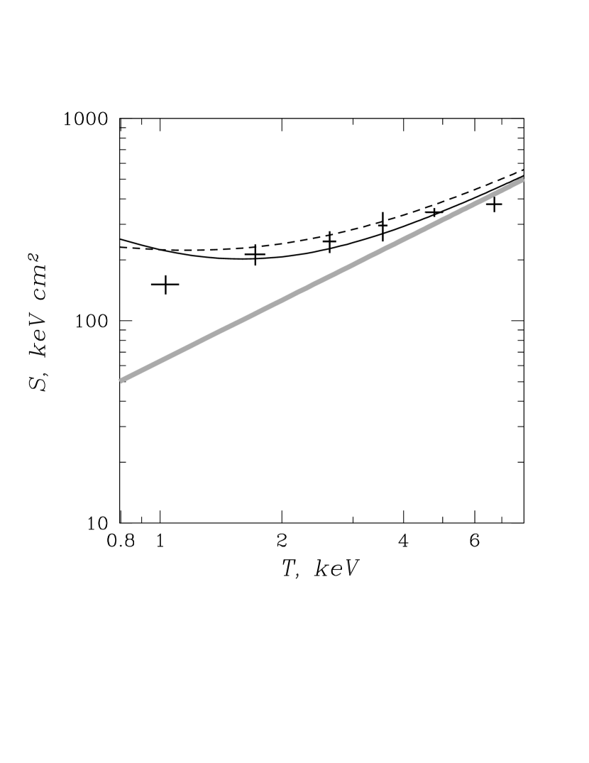
Figure 3.— Scaling relation between entropy ($S$), measured at 0.1 R₂₀₀, and temperature ($T$). The solid black line is the inferred relation accounting for a constant energy excess injected by radio galaxies (see text for details). The grey line is the expected self–similar relation. The points show the binned means from the observations by Ponman et al. (2003). The dashed line is the same as the solid line but considering the self–similar scaling M${}_{gas}\propto$T^1.5

7. Conclusions

In this Paper we have quantified the importance of the mechanical energy input by radio galaxies inside galaxy groups. In particular we report a striking difference between clusters and groups of galaxies: while the binding energy of the ICM in clusters exceeds the mechanical output by radio AGN, the two quantities are of the same order of magnitude in groups that host a radio galaxy within 0.15 R₂₀₀. This suggests that, while clusters can be mostly considered to be closed systems, the mechanical removal of gas is energetically possible from groups. This has implications that help explain recent findings on the baryonic fraction in groups of galaxies. Giodini et al. (2009) reported a $\sim$30$\%$ lack of gas in groups compared with the cosmological baryon mass fraction evaluated from the 5 years Wilkinson Microwave Anisotropy Probe (Dunkley et al., 2009). It has been suggested that this gas has been removed by AGN feedback.

This is consistent with cosmological models in which feedback from radio galaxies is invoked to successfully explain galaxy group/cluster properties. Based on a well selected sample of galaxy groups and clusters that host radio galaxies, we have observationally shown for the first time that this scenario is energetically feasible. We have further shown that a constant injection of excess energy by radio galaxy naturally reproduces the self-similar breaking observed in the scaling relation between the entropy and temperature of groups.

Appendix A Radio Images

Figure 4.— Figure 4 presents the contours maps of the radio 20 cm emission (magenta lines) superimposed to the SUBARU $zp$ band image for each of the groups listed in Table 1. Images are 3$\times$3 arcmin and centered on the group center, except XID246 which is 4$\times$4 arcmin wide and offset from the center group because of its location on the edge of the SUBARU field coverage. The white line shows the contours of X–ray flux significance. The contours correspond to $\left[3,6,9,12,15,18,21,24\right]\,\sigma$ X–ray flux significance.

$\begin{array}[]{c@{\hspace{1in}}c}\lx@intercol\mbox{}\hfil\lx@intercol&\lx@intercol\mbox{}\hfil\lx@intercol\\ \includegraphics[width=238.49121pt]{fig4}\hfil\hskip 72.26999pt&\includegraphics[width=238.49121pt]{fig5}\\[11.38092pt] \lx@intercol\mbox{}\hfil\lx@intercol&\lx@intercol\mbox{}\hfil\lx@intercol\\ \includegraphics[width=238.49121pt]{fig6}\hfil\hskip 72.26999pt&\includegraphics[width=238.49121pt]{fig7}\\[11.38092pt] \end{array}$

$\begin{array}[]{c@{\hspace{1in}}c}\lx@intercol\mbox{}\hfil\lx@intercol&\lx@intercol\mbox{}\hfil\lx@intercol\\ \includegraphics[width=238.49121pt]{fig8}\hfil\hskip 72.26999pt&\includegraphics[width=238.49121pt]{fig9}\\[11.38092pt] \lx@intercol\mbox{}\hfil\lx@intercol&\lx@intercol\mbox{}\hfil\lx@intercol\\ \includegraphics[width=238.49121pt]{fig10}\hfil\hskip 72.26999pt&\includegraphics[width=238.49121pt]{fig11}\\[11.38092pt] \end{array}$

$\begin{array}[]{c@{\hspace{1in}}c}\lx@intercol\mbox{}\hfil\lx@intercol&\lx@intercol\mbox{}\hfil\lx@intercol\\ \includegraphics[width=238.49121pt]{fig12}\hfil\hskip 72.26999pt&\includegraphics[width=238.49121pt]{fig13}\\[11.38092pt] \lx@intercol\mbox{}\hfil\lx@intercol&\lx@intercol\mbox{}\hfil\lx@intercol\\ \includegraphics[width=238.49121pt]{fig14}\hfil\hskip 72.26999pt&\includegraphics[width=238.49121pt]{fig15}\\[11.38092pt] \end{array}$

$\begin{array}[]{c@{\hspace{1in}}c}\lx@intercol\mbox{}\hfil\lx@intercol&\lx@intercol\mbox{}\hfil\lx@intercol\\ \includegraphics[width=238.49121pt]{fig16}\hfil\hskip 72.26999pt&\includegraphics[width=238.49121pt]{fig17}\\[11.38092pt] \lx@intercol\mbox{}\hfil\lx@intercol&\lx@intercol\mbox{}\hfil\lx@intercol\\ \includegraphics[width=238.49121pt]{fig18}\hfil\hskip 72.26999pt&\includegraphics[width=238.49121pt]{fig19}\\[11.38092pt] \end{array}$

References

- Arnaud & Evrard (1999) Arnaud, M., & Evrard, A. E. 1999, MNRAS, 305, 631
- Balogh et al. (2008) Balogh, M. L., McCarthy, I. G., Bower, R. G., & Eke, V. R. 2008, MNRAS, 385, 1003
- Baum et al. (1992) Baum, S. A., Heckman, T. M., & van Breugel, W. 1992, ApJ, 389, 208
- Bîrzan et al. (2004) Bîrzan, L., Rafferty, D. A., McNamara, B. R., Wise, M. W., & Nulsen, P. E. J. 2004, ApJ, 607, 800
- Bîrzan et al. (2008) Bîrzan, L., McNamara, B. R., Nulsen, P. E. J., Carilli, C. L., & Wise, M. W. 2008, ApJ, 686, 859
- Bower et al. (2006) Bower, R. G., Benson, A. J., Malbon, R., Helly, J. C., Frenk, C. S., Baugh, C. M., Cole, S., & Lacey, C. G. 2006, MNRAS, 370, 645
- Bower et al. (2008) Bower, R. G., McCarthy, I. G., & Benson, A. J. 2008, MNRAS, 390, 1399
- Chen et al. (2007) Chen, Y., Reiprich, T. H., Böhringer, H., Ikebe, Y., & Zhang, Y.-Y. 2007, A&A, 466, 805
- Churazov et al. (2002) Churazov, E., Sunyaev, R., Forman, W., & Böhringer, H. 2002, MNRAS, 332, 729
- Churazov et al. (2005) Churazov, E., Sazonov, S., Sunyaev, R., Forman, W., Jones, C., Boehringer, H. 2005, MNRAS, 363, L91
- Condon et al. (1998) Condon, J. J., Cotton, W. D., Greisen, E. W., Yin, Q. F., Perley, R. A., Taylor, G. B., & Broderick, J. J. 1998, AJ, 115, 1693
- Croton et al. (2006) Croton, D. J., et al. 2006, MNRAS, 365, 11
- De Young (2010) De Young, D. S. 2010, arXiv:1001.1178
- Donahue et al. (2005) Donahue, M., Voit, G. M., O’Dea, C. P., Baum, S. A., & Sparks, W. B. 2005, ApJ, 630, L13
- Drory et al. (2004) Drory, N., Bender, R., Feulner, G., Hopp, U., Maraston, C., Snigula, J., & Hill, G. J. 2004, ApJ, 608, 742
- Dunkley et al. (2009) Dunkley, J., et al. 2009, ApJS, 180, 306
- Evrard et al. (1996) Evrard, A. E., Metzler, C. A., & Navarro, J. F. 1996, ApJ, 469, 494
- Fabian et al. (1994) Fabian, A. C., Arnaud, K. A., Bautz, M. W., & Tawara, Y. 1994, ApJ, 436, L63
- Feretti & Giovannini (2007) arXiv:astro-ph/0703494v1
- Finoguenov et al. (2008) Finoguenov, A., Ruszkowski, M., Jones, C., Brüggen, M., Vikhlinin, A., & Mandel, E. 2008, ApJ, 686, 911
- Giodini et al. (2009) Giodini, S., et al. 2009, ApJ, 703, 982
- Gitti et al. (2007) Gitti, M., McNamara, B. R., Nulsen, P. E. J., & Wise, M. W. 2007, ApJ, 660, 1118
- Hayashi et al. (2007) Hayashi, E., Navarro, J. F., & Springel, V. 2007, MNRAS, 377, 50
- Heinz et al. (1998) Heinz, S., Reynolds, C. S., & Begelman, M. C. 1998, ApJ, 501, 126
- Ilbert et al. (2009) Ilbert, O., et al. 2009, ApJ, 690, 1236
- Kaastra et al. (2004) Kaastra, J. S., et al. 2004, A&A, 413, 415
- Kay (2004) Kay, S. T. 2004, MNRAS, 347, L13
- Lin et al. (2003) Lin, Y.-T., Mohr, J. J., & Stanford, S. A. 2003, ApJ, 591, 749
- Lloyd-Davies et al. (2000) Lloyd-Davies, E. J., Ponman, T. J., & Cannon, D. B. 2000, MNRAS, 315, 689
- Leauthaud et al. (2010) Leauthaud, A., et al. 2010, ApJ, 709, 97
- Macciò et al. (2007) Macciò, A. V., Dutton, A. A., van den Bosch, F. C., Moore, B., Potter, D., & Stadel, J. 2007, MNRAS, 378, 55
- Markevitch (1998) Markevitch, M. 1998, ApJ, 504, 27
- Myers & Spangler (1985) Myers, S. T., & Spangler, S. R. 1985, ApJ, 291, 52
- McCarthy et al. (2007) McCarthy, I. G., Bower, R. G., & Balogh, M. L. 2007, MNRAS, 377, 1457
- McNamara & Nulsen (2007) McNamara, B. R., & Nulsen, P. E. J. 2007, ARA&A, 45, 117
- Merloni & Heinz (2007) Merloni, A., & Heinz, S. 2007, MNRAS, 381, 589
- Navarro et al. (1996) Navarro, J. F., Frenk, C. S., & White, S. D. M. 1996, ApJ, 462, 563
- Nipoti & Binney (2005) Nipoti, C., & Binney, J. 2005, MNRAS, 361, 428
- Peres et al. (1998) Peres, C. B., Fabian, A. C., Edge, A. C., Allen, S. W., Johnstone, R. M., & White, D. A. 1998, MNRAS, 298, 416
- Peterson et al. (2001) Peterson, J. R., et al. 2001, A&A, 365, L104
- Peterson et al. (2003) Peterson, J. R., Kahn, S. M., Paerels, F. B. S., Kaastra, J. S., Tamura, T., Bleeker, J. A. M., Ferrigno, C., & Jernigan, J. G. 2003, ApJ, 590, 207
- Peterson & Fabian (2006) Peterson, J. R., & Fabian, A. C. 2006, Phys. Rep., 427, 1
- Ponman et al. (2003) Ponman, T. J., Sanderson, A. J. R., & Finoguenov, A. 2003, MNRAS, 343, 331
- Pratt & Arnaud (2003) Pratt, G. W., & Arnaud, M. 2003, A&A, 408, 1
- Pratt et al. (2009) Pratt, G. W., Croston, J. H., Arnaud, M., & Böhringer, H. 2009, A&A, 498, 361
- Pratt et al. (2009) Pratt, G. W., et al. 2009, arXiv:0909.3776
- Puchwein et al. (2008) Puchwein, E., Sijacki, D., & Springel, V. 2008, ApJ, 687, L53
- Reiprich & Boehringer (2002) Reiprich, T. H., Boehringer, H. 2002, ApJ, 567, 716
- Renzini (2006) Renzini, A. 2006, ARA&A, 44, 141
- Sanderson & Ponman (2003) Sanderson, A. J. R., & Ponman, T. J. 2003, MNRAS, 345, 1241
- Salvato et al. (2009) Salvato, M., et al. 2009, ApJ, 690, 1250
- Scoville et al. (2007a) Scoville, N., et al. 2007, ApJS, 172, 1
- Schinnerer et al. (2007) Schinnerer, E., et al. 2007, ApJS, 172, 46
- Sijacki & Springel (2006) Sijacki, D., & Springel, V. 2006, MNRAS, 366, 397
- Short & Thomas (2009) Short, C. J., & Thomas, P. A. 2009, ApJ, 704, 915
- Skrutskie et al. (2006) Skrutskie, M. F., et al. 2006, AJ, 131, 1163
- Smolčić et al. (2008) Smolčić, V., et al. 2008, ApJS, 177, 14
- Smolčić et al. (2009) Smolcic, V., et al. 2009, arXiv:0901.3372
- Sun et al. (2009) Sun, M., Voit, G. M., Donahue, M., Jones, C., Forman, W., & Vikhlinin, A. 2009, ApJ, 693, 1142
- Voigt & Fabian (2004) Voigt, L. M., & Fabian, A. C. 2004, MNRAS, 347, 1130
- Voit (2005) Voit, L. M. 2005, Reviews of Modern Physics, 77, 207
- Voit & Donahue (2005) Voit, G. M., & Donahue, M. 2005, ApJ, 634, 955
- Wright & Otrupcek (1990) Wright, A., & Otrupcek, R. 1990, PKS Catalog (1990), 0