Quantum Hall Phase Diagram of Half-filled Bilayers in the Lowest and the Second Orbital Landau Levels: Abelian versus Non-Abelian Incompressible Fractional Quantum Hall States

Abstract

We examine the quantum phase diagram of the fractional quantum Hall effect (FQHE) in the lowest two Landau levels in half-filled bilayer structures as a function of tunneling strength and layer separation, i.e., we revisit the lowest Landau level filling factor 1/2 bilayer problem and make predictions involving bilayers in the half-filled second Landau level (i.e., filling factor 5/2). Using numerical exact diagonalization we investigate the important question of whether this system supports a FQHE described by the non-Abelian Moore-Read Pfaffian state in the strong tunneling regime. In the lowest Landau level, we find that although in principle, increasing (decreasing) tunneling strength (layer separation) could lead to a transition from the Abelian two-component Halperin 331 to non-Abelian one-component Moore-Read Pfaffian state, the FQHE excitation gap is relatively small in the lowest Landau level Pfaffian regime, and we establish that all so far observed FQHE states in half-filled lowest Landau level bilayers are most likely described by the Abelian Halperin 331 state. In the second Landau level we make the prediction that bilayer structures would manifest two distinct branches of incompressible FQHE corresponding to the Abelian 331 state (at moderate to low tunneling and large layer separation) and the non-Abelian Moore-Read Pfaffian state (at large tunneling and small layer separation). The observation of these two FQHE branches and the possible quantum phase transition between them will be compelling evidence supporting the existence of the non-Abelian Moore-Read Pfaffian state in the second Landau level. We discuss our results in the context of existing experiments and theoretical works.

I Introduction

Two important developments have rekindled interest in the phenomena of even-denominator incompressible fractional quantum Hall states in two-dimensional high-mobility bilayer semiconductor structures. The first is the recent intriguing experimental observation by Luhman et al. Luhman et al. (2008) of two distinct even-denominator fractional quantum Hall effect (FQHE) states at filling factors $\nu=1/2$ and 1/4 in a very wide ($\sim 600\AA$) single quantum well (wide-quantum-well) structure at very high ($>40T$) magnetic fields. The second development, motivated by implications for fault-tolerant topological quantum computation Das Sarma et al. (2005); Nayak et al. (2008), is the great deal of recent theoretical and experimental interest in the possible non-Abelian nature of the $\nu=5/2$ second Landau level (SLL) FQHE state first observed by Willett et al. Willett et al. (1987) in the single-layer system in 1987 with subsequent confirming observations Eisenstein et al. (1988); Gammel et al. (1988); Pan et al. (1999); Eisenstein et al. (2002); Xia et al. (2004); Csáthy et al. (2005); Choi et al. (2008) over the years since. The FQHE at filling factor $\nu=5/2$ presents an amazing confluence of ideas from condensed matter physics, conformal field theory, topology, and quantum computation. Nayak et al. (2008) In particular, the fundamental nature of the experimentally observed 5/2 FQHE, whether an exotic spin-polarized non-Abelian incompressible paired state or a more common Abelian incompressible paired state, has remained an enigma for more than 20 years. Although theoretical and numerical work indicates that the 5/2 FQHE belongs to a non-Abelian Moore-Read Pfaffian Moore and Read (1991) universality class, there is scant experimental evidence supporting this conclusion Dean et al. (2008) (see Ref. Nayak et al., 2008 for a comprehensive review of non-Abelian physics and topological quantum computation).

These two developments lead to important and interesting questions. One question is whether a non-Abelian $\nu=1/2$ FQHE, i.e., the analog of the possibly non-Abelian $\nu=5/2=2+1/2$ SLL single-layer state foo (a), can exist in the lowest Landau level (LLL) under experimentally observable conditions. This question has a long history He et al. (1991); Greiter et al. (1992); He et al. (1993); Nomura and Yoshioka (2004) in the theoretical literature going back to the early 1990s and recent FQHE experiments at $\nu=1/2$ make it imperative that a theoretical analysis be carried out to achieve a proper qualitative understanding of current experiments Luhman et al. (2008); Shabani et al. (2009a).

Another important question concerns the non-Abelian-ness (or not) of the experimental 5/2 state which is of profound importance beyond quantum Hall physics Das Sarma et al. (2005); Nayak et al. (2008). Hence, it is useful to contemplate novel situations where the nature of the 5/2 state will manifest itself in a dramatic, but hitherto unexplored, manner. The current work addresses the dichotomy (i.e., the 1/2 FQHE being an Abelian Halperin 331 bilayer state Halperin (1983) versus the 5/2 FQHE being a non-Abelian Moore-Read Pfaffian Moore and Read (1991); Read and Rezayi (1996) single-layer state) between single-layer SLL physics versus bilayer LLL physics by studying the bilayer FQHE in both the lowest and second LLs as a function of layer separation and tunneling. We ask whether bilayers can support both Pf and 331 FQHE.

The proposed non-Abelian Moore-Read Pfaffian (Pf) state is a weak-pairing single-layer (or one-component) FQHE state for half-filled LLs which, in principle, applies to any orbital LL (i.e., LLL as well as SLL). Thus, as a matter of principle a $\nu=1/2$ LLL single-layer Pf FQHE is certainly a possibility He et al. (1993); Storni et al. (2008); Papić et al. (2009); Nomura and Yoshioka (2004); Greiter et al. (1992); Shabani et al. (2009b) although it has never been observed experimentally. Theoretically, due to the differences in the electron-electron Coulomb interaction pseudo-potentials in the LLL compared to the SLL the two situations (i.e., 1/2 and 5/2) are quantitatively very different, and it is possible for the Pf FQHE to exist in the SLL, but not in the LLL (and vice versa). The best existing numerical work Peterson et al. (2008a); Papić et al. (2009); Papić et al. (2009); Storni et al. (2008) indicates that either the single-layer $\nu=1/2$ LLL Pf state does not exist in nature or if it exists, does so only in rather thick 2D layers with an extremely small FQHE excitation gap, making it impossible or very difficult to observe experimentally. By contrast, the single-layer $\nu=5/2$ SLL FQHE is observed routinely, albeit at low temperatures ($\lesssim 100mK$), in high mobility ($\gtrsim 10^{7}cm^{2}/Vs$) samples, and with a rather small (but experimentally accessible) activation gap ($\sim 100$-$500mK$). In fact, it has been pointed out that the experimental $\nu=5/2$ FQHE is always among the strongest observed FQHE states in the SLL.

Instead of studying a single-layer 2D system, we concentrate on the spin-polarized and density balanced bilayer system assuming an arbitrary tunneling strength $t$ and an arbitrary layer separation $d$ in the lowest and second LLs. We confine our study to spin-polarized systems because all experimentally realized half-filled FQHE states appear to be fully spin-polarized, consistent with the theoretical expectation Morf (1998); Feiguin et al. (2009)–whether bilayer two-component FQHE states at $\nu=1/2$ or one-component single-layer FQHE states at $\nu=5/2$. By density “balanced” we mean that each layer in the bilayer system has the same number of electrons. Furthermore, it should be noted that the tunneling strength $t$ is proportional to the symmetric-antisymmetric energy gap. The experimentally realizable system we have in mind could either be a true bilayer double-quantum-well structure or a single wide-quantum-well (WQW) which manifests effective bilayer behavior where the self-consistent field from the electrons produces effective two-component behavior Luhman et al. (2008); Shabani et al. (2009a) (see Fig. 18 in Sec. VIII).

We numerically obtain the approximate quantum phase diagram for a 1/2 filled bilayer system in either the lowest or second Landau level in the $t$-$d$ space using the spherical system finite size exact diagonalization (Lanczos) technique, concentrating entirely on the Pf and the 331 FQHE phases.

For the LLL, we revisit the $\nu=1/2$ bilayer FQHE and carry out an extensive comparison with all existing bilayer $\nu=1/2$ FQHE experimental observations to ascertain any hint of the existence of a non-Abelian Moore-Read Pfaffian state for large values of $t$. No strictly single-layer system, e.g., a heterostructure or a not-too-thick quantum well, has ever demonstrated an incompressible FQHE at $\nu=1/2$, instead manifesting only the compressible composite fermion Jain (1989, 2007) Fermi sea Kalmeyer and Zhang (1992); Halperin et al. (1993). It is intuitive that our model system is an effective bilayer, or single-layer, $\nu=1/2$ system for small, or large, values of $t$, and therefore by studying the quantum phase diagram as a function of $t$ and $d$ we hope to shed light on the possible existence of a single-layer $\nu=1/2$ FQHE in real systems.

One of the results of the current work is that for the lowest Landau level bilayer FQHE system, (i) the recently observed WQW $\nu=1/2$ FQHEs Luhman et al. (2008); Shabani et al. (2009a) are strong-pairing Abelian Halperin 331 FQHE states Halperin (1983, 1994) which, however, sit close to the boundary between the Abelian 331 and the weak-pairing non-Abelian Pfaffian FQHE state Moore and Read (1991), and (ii) it may be conceivable, as a matter of principle, to realize the LLL $\nu=1/2$ Pfaffian non-Abelian FQHE in very thick bilayers, but as a matter of practice, this is unlikely since the $\nu=1/2$ FQHE gap is extremely small (perhaps zero) in the parameter regime where the Pf is more stable than the 331 phase. Our findings about the fragility of the LLL $\nu=1/2$ non-Abelian Pf state are consistent with recent conclusions Peterson et al. (2008a); Papić et al. (2009); Papić et al. (2009); Storni et al. (2008), but our main focus in the current work is in understanding the $\nu=1/2$ bilayer quantum phase diagram treating tunneling $t$, layer separation $d$, and individual layer width $w$ of the 2D system as independent tuning parameters of the Hamiltonian.

For the second Landau level, we predict that bilayers can support both the non-Abelian Moore-Read Pfaffian and the Halperin Abelian 331 FQHE and that there could be a novel quantum phase transition, both as a function of tunneling strength (at constant layer separation) and of layer separation (at constant tunneling), between the two-component 331 Abelian and the one-component Pf non-Abelian states in a bilayer SLL system. We show that tuning the inter-layer tunneling and/or layer separation would lead to a transition between the Abelian and the non-Abelian SLL FQHE, which should be observable experimentally in standard FQHE transport experiments. In particular, we predict that in realistic systems with finite single-layer width, the SLL bilayer state would manifest two distinct FQHE phases separated by a region of finite inter-layer separation and tunneling. Existence of two distinct incompressible FQHE bilayer states at total filling factor $\nu=5/2$, connected possibly by a quantum phase transition, is a clear (experimentally testable) prediction of our theory. The observation of such a quantum phase transition, originally predicted as possible by Read and Green Read and Green (2000) (Fig. 1 in Ref. Read and Green, 2000) under general theoretical considerations (but never before demonstrated to be feasible under realistic conditions), would strongly suggest the existence of a non-Abelian 5/2 state since the two distinct FQHE phases in the same sample both cannot conceivably be Abelian 331 states.

We first present a background for our work in Section II and then describe our theoretical model in terms of a Hamiltonian and introduce all relevant parameters in Section III. Next we revisit the lowest Landau level problem in Section IV before tackling the second Landau level problem in Section V, since the LLL problem, due to its long history, is easier to understand and will provide a proper context and atmosphere when discussing our SLL results. In Section IV.3 we discuss in detail how we connect our results with current and previous experimental FQHE bilayer LLL results. Furthermore, in Section  V.4 we discuss am important issue regarding bilayer FQHE systems in higher Landau levels–a difficulty or ambiguity that is quite subtle and has not been discussed previously as far as we know. Lastly we present our conclusions in Section VI.

II Background

Before describing and presenting our work, it is useful to provide a brief background of bilayer FQHE, a subject with a long history, in order to set a context for our work.

The two candidate wavefunctions we consider and compare in this work, with respect to $\nu=1/2$ and 5/2 bilayer incompressible states, the Halperin 331 state Halperin (1983, 1994) and the Moore-Read Pfaffian state Moore and Read (1991) were proposed in 1983 and 1991, respectively. The 331 wavefunction is a two-component strongly paired Abelian state of two Laughlin Laughlin (1983) phases in each layer whereas the Pfaffian is a one-component weak pairing non-Abelian superconducting state of chiral $p$-wave symmetry. Both of these states are allowed incompressible fractional quantum Hall (FQH) phases at half-filled Landau levels which for our purpose could be either $\nu=1/2$ or 5/2($=2+1/2$). The qualitative difference between these two incompressible FQH states is that the 331 is an Abelian two-component state whereas the Pfaffian is a non-Abelian one-component state.

It was first explicitly shown by Yoshioka, Girvin, and MacDonald Yoshioka et al. (1988, 1989) that a bilayer system at (total) half-filling could support a 331 incompressible state for a layer separation $d\sim l$ (where $l$ is a characteristic length scale called the magnetic length, defined below), i.e., when intra- and inter-layer correlations are comparable. Later, He et al. He et al. (1991, 1993) carried out a detailed quantitative analysis of the possible existence of 331 FQHE in $\nu=1/2$ bilayer structures, making specific predictions for layer separation ($d$) and layer width ($w$) values where experimentally observable incompressible states may exist. This lead to the observation of $\nu=1/2$ bilayer 331 FQHE by Eisenstein et al. Eisenstein et al. (1992). Parallel to the Eisenstein et al. observation of the 331 FQHE in bilayers, Shayegan et al. Suen et al. (1992a, b) observed a well-defined $\nu=1/2$ FQHE in wide-quantum-wells. This WQW observation of $\nu=1/2$ FQHE was at first attributed to the one-component Moore-Read Pfaffian state by Greiter, Wen, and Wilczek Greiter et al. (1992), who argued that the occurance of a $\nu=1/2$ FQHE in a single quantum well, rather than in double quantum wells, implies a one-component rather than two-component nature of the underlying incompressible state. Later theoretical work by He et al. He et al. (1993) and further experimental work by Shayegan et al. Suen et al. (1992b, 1994) decisively established that the wide-well $\nu=1/2$ FQHE is, in fact, a manifestation of the two-component 331 rather than the one-component Pfaffian state. The existence of a two-component 331 FQHE in wide single wells becomes possible by virtue of the self-consistent Hartree electric field arising from the electrons themselves which, for sufficiently large quantum well width ($W$) and carrier density ($n$), could lead to the single wide-quantum-well acting effectively as two distinct electron layers localized near the well boundaries (with density $n/2$ each) with a potential barrier separating them in the middle. Such a two-component 331 FQHE description of observed $\nu=1/2$ incompressibility has become well-accepted, and the fact that no $\nu=1/2$ FQHE has ever been observed in relatively thin single quantum well structures or in single heterostructures has further reinforced the idea that the $\nu=1/2$ FQHE is due to the formation of the two-component Halperin 331 state in wide-quantum-wells r (1).

From the perspective of $\nu=1/2$ FQHE, wide-quantum-wells should be considered as two-component bilayer systems with non-zero interlayer tunneling. For relatively weak, or strong, tunneling between the layers, the system behaves as a two, or one, component system, and the question of the existence of Abelian 331 or non-Abelian Pfaffian $\nu=1/2$ FQHE then, in some sense, boils down to the existence of incompressible FQHE in the weak or strong tunneling limit. Unfortunately, how strong an interlayer tunneling is strong enough to render the system into a one-component Pfaffian FQHE is a quantitative question, which can only be addressed through detailed numerical study. Such a numerical study is the main goal of this paper. In the process, we also ask the question of one-component versus two-component (i.e., Pfaffian versus 331) FQHE in bilayer $\nu=5/2$ case, where the existence of the one-component Pfaffian $\nu=5/2$ FQHE is reasonably well-established theoretically Morf (1998); Rezayi and Haldane (2000); Park et al. (1998); Scarola et al. (2002, 2000); Peterson et al. (2008b, a); Möller and Simon (2008), although actively debated Tőke and Jain (2006); Tőke et al. (2007); Wójs and Quinn (2006). The bilayer $\nu=5/2$ case was never studied before in the literature whereas there were only two studies of the bilayer $\nu=1/2$ case comparing 331 versus Pfaffian state. The first is by He et al. He et al. (1993) and the second is by Nomura and Yoshioka Nomura and Yoshioka (2004). Our work for $\nu=5/2$ is distinct, and our work for $\nu=1/2$ transcends that of the earlier work in being much more complete. Very recently, Papić et al. Papić et al. (2009) investigated this problem using a somewhat different model.

As mentioned in the Introduction (Sec. I), our work is partially motivated by the recent experimental observation of Luhman et al. Luhman et al. (2008) who found a $\nu=1/2$ FQHE in side single wells with relatively strong tunneling (i.e., large symmetric-antisymmetric energy splitting). An interesting question is whether the $\nu=1/2$ FQHE observed in the Luhman et al. experiment is a two-component 331 state or a one-component Pfaffian state. We do not study the $\nu=1/4$ FQHE observed by Luhman et al. which has recently been discussed by Papić et al. Papić et al. (2009)

We mention that all our theoretical work assumes complete spin-polarization of the electrons and considers only the balanced case where the average electron density is the same in each layer. We also neglect all Landau level coupling effects, and as such our work does not distinguish between the non-Abelian Pfaffian and the non-Abelian anti-Pfaffian Levin et al. (2007); Lee et al. (2007); Peterson et al. (2008c); Wang et al. (2009) states at $\nu=1/2$ or 5/2. (Note that the neglect of LL mixing effects may not be a particularly good assumption for the 5/2 FQHE Dean et al. (2008); Bishara and Nayak (2009).) The reason for our considering full spin-polarization is that prior theoretical work by Morf Morf (1998) and by Feiguin et al. Feiguin et al. (2009) indicates that the $\nu=1/2$ or 5/2 state is likely to be fully spin-polarized. If the bilayer incompressible states turn our to be unpolarized or partially polarized, our work simply would not be valid.

With this background, we study the stability of the 331 and the Pfaffian state in $\nu=1/2$ and 5/2 bilayers in the presence of finite interlayer tunneling ($t$), interlayer separation ($d$), and layer width ($w$). Our goal is to obtain an appropriate zeroth-order quantum phase diagram in the $t$-$d$-$w$ space for $\nu=1/2$ and 5/2 bilayer FQHE. Given that we calculate and compare the exact many-body ground state for many individual values of $t$, $d$, and $w$, we are forced to use a rather modest system size for $N=8$ electrons (i.e., 4 in each layer) in all our exact diagonalization work. Past experience shows that a 8-electron system is quit adequate for qualitative understanding as long as precise thermodynamic values of excitation gap or ground state energy are not desired.

III Theoretical Model

We use the simplest model Hamiltonian $\hat{H}$ incorporating both finite tunneling $t$ and finite layer separation $d$ (as well as finite layer width $w$–or finite thickness) for our bilayer FQHE system:

$$\hat{H}=\sum_{i<j}^{N}[V_{\mathrm{intra}}(|\mathbf{r}_{i}-\mathbf{r}_{j}|)+V_{\mathrm{intra}}(|\tilde{\mathbf{r}}_{i}-\tilde{\mathbf{r}}_{j}|)+V_{\mathrm{inter}}(|\mathbf{r}_{i}-\tilde{\mathbf{r}}_{j}|)]-t(\hat{S}_{x})_{\mathrm{layer}}\;,$$ (1)

$\mathbf{r}_{i}$ and $\tilde{\mathbf{r}}_{i}$ are the position of the $i$-th electron in the right and left layer, respectively. In Eq. (1), $V_{\mathrm{intra}}(r)=e^{2}/(\kappa\sqrt{r^{2}+w^{2}})$ (we use the Zhang-Das Sarma Zhang and Das Sarma (1986) potential to model the single layer quasi-2D interaction) and $V_{\mathrm{inter}}(r)=e^{2}/(\kappa\sqrt{r^{2}+d^{2}})$ are the intralayer and interlayer Coulomb interaction incorporating a finite layer width $w$ and a center-to-center interlayer separation $d$ ($>w$ by definition). The $x$-component of the pseudo-spin operator $(\hat{S}_{x})_{\mathrm{layer}}$ (written in the layer basis representation) controls the tunneling between the two quantum wells with large $t$ denoting strong tunneling.

Note that in the bilayer problem when the electron density is balanced in each layer, i.e., total number of particles in each layer is $N/2$, there are essentially two natural Hilbert space representations. The layer basis (in which Eq. 1 is written) or the symmetric-antisymmetric basis where $c_{mS}=(c_{mR}+c_{mL})/\sqrt{2}$ and $c_{mA}=(c_{mR}-c_{mL})/\sqrt{2}$ destroy an electron in the symmetric ($S$) and antisymmetric ($A$) superposition states, respectively, where $m$ is angular momentum and $c_{mR}$ and $c_{mL}$ destroy an electron in the right and left quantum well, respectively. $S(A)$ can be considered to be an effective pseudo-spin index for the bilayer system. In the symmetric-antisymmetric basis, the Hamiltonian is written as

$$\hat{H}=\frac{1}{2}\sum_{\{m_{i},\sigma_{i}=A,S\}}\langle m_{1}\sigma_{1},m_{2}\sigma_{2}|V|m_{4}\sigma_{4},m_{3}\sigma_{3}\rangle c^{\dagger}_{m_{1}\sigma_{1}}c^{\dagger}_{m_{2}\sigma_{2}}c_{m_{4}\sigma_{4}}c_{m_{3}\sigma_{3}}-\frac{t}{2}\sum_{m}(c^{\dagger}_{mS}c_{mS}-c^{\dagger}_{mA}c_{mA})\;.$$ (2)

As written above in Eq. 1, the intra-layer Coulomb potential energy between two electrons is $V=V_{\mathrm{intra}}$ and the inter-layer potential energy is $V=V_{\mathrm{inter}}$. A difference between the two representations is that the tunneling operator in the layer-basis can be written as $(\hat{S}_{x})_{\mathrm{layer}}$ while, in the symmetric-antisymmetric basis, the tunneling operator is $(\hat{S}_{z})_{SAS}=\frac{1}{2}\sum_{m}(c^{\dagger}_{mS}c_{mS}-c^{\dagger}_{mA}c_{mA})=\frac{1}{2}\sum_{m}(c^{\dagger}_{mR}c_{mL}+c^{\dagger}_{mL}c_{mR})=(\hat{S}_{x})_{\mathrm{layer}}$. The layer- and symmetric-antisymmetric-bases are related through a pseudo-spin rotation. Of course, the choice is a matter of personal taste and convenience and one should really appeal to a physical explanation to understand the tunneling: no matter the basis choice, the tunneling term controls the probability that electrons jump back and forth between the two layers keeping the total number of electrons in each layer fixed at $N/2$, i.e., keeping the bilayer system density balanced.

We numerically diagonalize $\hat{H}$ for finite $N$ assuming specific values of $w$, $d$, and $t$ (each expressed throughout in dimensionless units using the magnetic length $l=(c\hbar/eB)^{1/2}$ as the length unit and the Coulomb energy $e^{2}/(\kappa l)$, where $\kappa$ is the background dielectric constant of the host semiconductor, as the energy unit; $e$ is electron charge, $c$ is the speed of light in vacuum, and $B$ is the magnetic field strength). We utilize the spherical geometry where the electrons are confined to a spherical surface of radius $R=\sqrt{N_{\phi}/2}$, $N_{\phi}$ is the total magnetic flux piercing the surface ($N_{\phi}$ is an integer according to Dirac), and the filling factor in the partially occupied Landau level (whether LLL or SLL) is $\lim_{N\rightarrow\infty}N/N_{\phi}$ . To fully consider tunneling, the Hilbert space must contain basis states with $\tilde{N}$ and $N-\tilde{N}$ electrons in the right and left layers for $\tilde{N}\in[0,N]$.

Following the standard well-tested procedures He et al. (1991); Greiter et al. (1992); He et al. (1993); Nomura and Yoshioka (2004); Peterson et al. (2008a); Papić et al. (2009); Papić et al. (2009); Storni et al. (2008) used extensively in the FQHE literature, we calculate the overlap between the exact numerical $N$ electron ground state wavefunction of the Coulomb Hamiltonian defined by Eq. (1) and the candidate $N$ electron variational states which are the Abelian Halperin 331 strong-pairing Halperin (1983) and the non-Abelian Moore-Read Pfaffian weak-pairing Moore and Read (1991) wavefunctions:

$$\Psi_{331} = \prod_{i<j}^{N/2}(z_{i}-z_{j})^{3}\prod_{i<j}^{N/2}(\tilde{z}_{i}-\tilde{z}_{j})^{3}\prod_{i,j}^{N}(z_{i}-\tilde{z}_{j})$$ (3)

$$\Psi_{\mathrm{Pf}} = \mathrm{Pf}\left\{\frac{1}{z_{i}-z_{j}}\right\}\prod_{i<j}^{N}(z_{i}-z_{j})^{2}\;,$$ (4)

respectively, where $z=x-iy$ is the electron coordinate in the $x$-$y$ plane. Intuitively, the “331” in $\Psi_{331}$ originates from the exponents for $(z_{i}-z_{j})$, $(\tilde{z}_{i}-\tilde{z}_{j})$, and $(z_{i}-\tilde{z}_{j})$, respectively, i.e., 3, 3, and 1. (Note that other Halperin 331-type wavefunctions Möller et al. (2008, 2009) have been considered for other filling factors, e.g., total $\nu=1$, and recently the total $\nu=5/2+5/2=5$ bilayer FQHE has been considered shi , however, none of these states directly apply to the situation that we are investigating of a half-filled LLL or SLL.) Both $\Psi_{331}$ and $\Psi_{\mathrm{Pf}}$ are written above in the layer representation, where the 331 state pairs electrons between layers and $\Psi_{\mathrm{Pf}}$ pairs electrons in a single-layer, since writing the wavefunctions in real space and appealing to the layer basis representation is much more intuitive. However, we are working within the “balanced” density situation so the Pf wavefunction, in particular, should be thought of as a wavefunction that describes pairing among electrons in the symmetric state (($c_{mR}+c_{mL})/\sqrt{2}$) since the electrons are never physically completely in a single layer, right or left.

We emphasize that we only consider the above two candidate wavefunctions. It is well known Kalmeyer and Zhang (1992); Halperin et al. (1993) that a composite fermion liquid phase (or composite fermion Fermi sea) exists for $\nu=1/2$ one-component systems both from extensive theoretical analysis and experimental observations Jain (2007). On the other hand, it is strongly suspected that for one-component systems at $\nu=5/2$, the ground state is the Moore-Read Pfaffian phase. Again, this is known from theoretical and experimental works Morf (1998); Rezayi and Haldane (2000); Scarola et al. (2002); Peterson et al. (2008b, a); Möller and Simon (2008). There are other candidate wavefunctions that can be written down besides $\Psi_{331}$ and $\Psi_{\mathrm{Pf}}$. Namely, one could consider $\Psi_{222}$ and $\Psi_{440}$ (both obvious generalizations of naming convention used for $\Psi_{331}$) that describe a pseudo-spin unpolarized composite fermion Fermi sea and two uncorrelated one-quarter-filled composite fermion Fermi seas, respectively Jain (2007). However, those states have different “shifts” (see below) in the spherical geometry than one another and $\Psi_{331}$ and $\Psi_{\mathrm{Pf}}$ and cannot be compared on an equal footing foo (b) and comparing them each to the exact state $\Psi_{0}$ would require many additional calculations that are simply beyond the scope of this work.

After diagonalizing $\hat{H}$ we ensure that (i) the ground state is homogeneous, i.e., has total orbital angular momentum $L=0$ and is therefore an incompressible state, and (ii) there is a gap, the FQHE excitation gap, separating the ground state from all excited states. We are concerned with the Pf and 331 variational states for total filling factor 1/2 in either the lowest or second Landau level, so $N_{\phi}=2N-3$, the “-3” is known as the “shift” and is a consequence of the curvature of the spherical geometry in which we work. Throughout, we consider $(N,N_{\phi})=(8,13)$ and mention that due to the pseudo-spin component present in the bilayer problem the Hilbert space is large (more than $10^{5}$ states for $N=8$ and over $7\times 10^{6}$ for $N=10$). Usually when one is utilizing exact diagonalization one wishes to consider many different system sizes and extrapolate the finite size results to the infinite system size through some sort of finite-size scaling. The computational difficulty of our problem does not allow this. $N=6$ electrons at $N_{\phi}=2N-3$ is aliased with a one-component FQHE corresponding to $\nu=2/3$–remember the filling factor $\nu=\lim_{N\rightarrow\infty}N/N_{\phi}$, so for certain combinations of $N$ and $N_{\phi}$ there can be correspondence between the finite systems and two distinct filling factors (the so-called aliasing problem). Hence, the $N=6$ case will produce ambiguous results (and, in fact, this aspect raises some questions about the work of Nomura and Yoshioka Nomura and Yoshioka (2004) who used $N=6$ to do a similar investigation for $\nu=1/2$ bilayers). $N=10$ is too big for us to exactly diagonalize (mentioned above) so we are left with only being able to consider $N=8$ and no finite size scaling is possible. Although this is a drawback, it is not uncommon in theoretical FQHE studies to use a modest system size, but many different sets of physical parameters (i.e., $t$, $d$, $w$ for our case) to bring out qualitative features. Furthermore, since the theoretical techniques are standard, we do not give the details, concentrating instead on the results and their implications for bilayer FQHE experiments.

We investigate this system with the usual probes used in theoretical FQHE studies by calculating: (i) wavefunction overlap between variational ansatz ($\Psi_{\mathrm{Pf}}$ and $\Psi_{331}$ states) and the exact ground state $\Psi_{0}$ of $\hat{H}$–an overlap of unity or zero indicates that the physics is or is not described by the ansatz; (ii) expectation value of the exact ground state of $(N_{S}-N_{A})/2$ , where $N_{S}$ and $N_{A}$ are the expectation values of the number of electrons in the symmetric or the antisymmetric states, respectively–a value of zero or $N/2$ indicating the ground state to be two- or one-component; and (iii) energy gap (provided the ground state is a uniform state with $L=0$)–a non-zero excitation gap indicating a possible FQHE state. In other words, we ask: (i) What is the physics (i.e., 331 or Pf)?; (ii) Is the system one- or two-component?; (iii) Will the system display FQHE (i.e., is the system compressible or incompressible)?

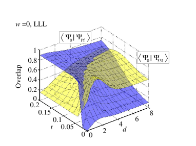
(a) (b)

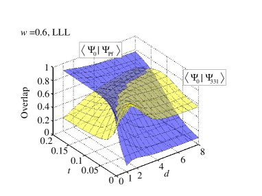
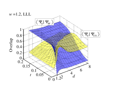
(c) (d)

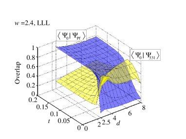
Figure 1: (Color online) Wavefunction overlap between the exact ground state, $\Psi_{0}$, and the Pf state, $\Psi_{\mathrm{Pf}}$ (blue (dark gray)), and 331 state, $\Psi_{331}$ (yellow (light gray)), as a function of layer separation $d$ and tunneling amplitude $t$ for the $\nu=1/2$ lowest LL with $N=8$ electrons and single layer width (a) $w=0$, (b) $w=0.6$, (c) $w=1.2$, and (d) $w=2.4$ ($d\geq w$ necessarily).

The calculated overlap and gap determine the nature of the FQHE and its strength in our theory. We operationally define the system to be in the 331 or Pf phase depending on whether the overlap between the exact ground state and the 331 or Pf wavefunctions is larger, i.e., if $\langle\Psi_{0}|\Psi_{331}\rangle>\langle\Psi_{0}|\Psi_{\mathrm{Pf}}\rangle$ then the system is said to be in the 331 phase and vice versa. We emphasize that our work is a comparison between these two incompressible states only, and we cannot comment on the possibility of some other state (i.e., neither 331 nor Pf) being the ground state. We do, however, believe that if the system is incompressible at a particular set of parameter values (i.e., $d$, $t$, $w$, etc.), it is very likely to be described by one of these two candidate states, 331 or Pf. We cannot, however, rule out the possibility that the real system has a compressible ground state (without manifesting FQHE), e.g., a composite fermion Fermi sea, not considered in our calculation. This is more likely to happen when our calculated excitation gap is very small.

IV Lowest Landau Level Results

IV.1 What is the physics?–lowest Landau level

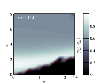
(a) (b)

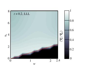
Figure 2: (Color online) Wavefunction overlap between the exact ground state $\Psi_{0}$ and $\Psi_{\mathrm{Pf}}$ at strong tunneling $t=0.2$ (a) and $\Psi_{331}$ at zero tunneling $t=0$ (b) as a function of separation $d$ and single-layer well width $w$ (where $d\geq w$) for the $\nu=1/2$ lowest LL with $N=8$ electrons. White corresponds to an overlap of unity while black corresponds to an overlap of zero. The dashed red line is the condition $w=d$ and for $w>d$ the bilayer system is undefined, i.e., the single-layer width cannot be larger than the layer separation.

The calculated wavefunction overlap between the exact ground state $\Psi_{0}$ and the two appropriate candidate variational wavefunctions ($\Psi_{\mathrm{Pf}}$ and $\Psi_{331}$) as a function of distance $d$ and tunneling energy $t$ is shown in Fig. 1. First we focus on the situation with zero width $w=0$ (Fig. 1(a)) and concentrate on the overlap with $\Psi_{\mathrm{Pf}}$. In the limit of zero tunneling and zero separation, the overlap with $\Psi_{\mathrm{Pf}}$ is zero and quickly jumps to approximately 0.9 when the tunneling is increased to only a small amount of approximately 0.025, and for increasing tunneling, $\langle\Psi_{0}|\Psi_{\mathrm{Pf}}\rangle$ remains relatively constant. In fact, this zero $d$ and large tunneling result should be compared to the single layer results we have given earlier (Fig. 9(a) in Ref. Peterson et al., 2008a). For $d\neq 0$, in the weak tunneling limit the overlap with $\Psi_{\mathrm{Pf}}$ remains very small. However, in the large tunneling limit, increasing $d$ only reduces the overlap marginally and the Pf description remains quite good even for large $d$. This shows that the strong-tunneling (one-component) regime is well described by the Pf state. It should be noted, however, that the overlap between $\Psi_{0}$ and $\Psi_{\mathrm{Pf}}$ is never much above 0.9–this should be compared to the SLL where we know Morf (1998); Rezayi and Haldane (2000); Scarola et al. (2002); Peterson et al. (2008b, a); Möller and Simon (2008); Storni et al. (2008) that the Pf wavefunction is a good physical description in the small layer separation and large tunneling limit (see Section V.1).

Next we consider the overlap between $\Psi_{0}$ and $\Psi_{331}$. In the zero tunneling limit, as a function of $d$, we find the overlap starts very small, increases to a moderate maximum of $\approx 0.80$ at $d\sim 1$ before achieving an essentially constant value of $\approx 0.6$. For $d>4$ the overlap increases with increasing tunneling to a maximum of nearly 0.8. Thus, the weak-tunneling (two-component) regime is well described by $\Psi_{331}$ and the 331 state is very robust to tunneling when layer separation is large. For small layer separation ($d<2$), non-zero tunneling very quickly suppresses the overlap between $\Psi_{331}$ and the exact state to a very small value.

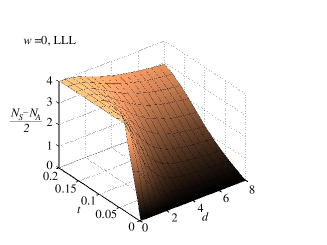
(a) (b)

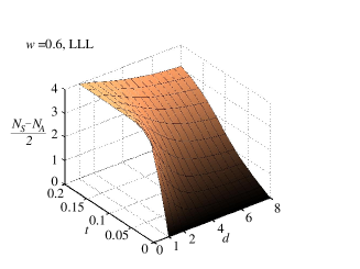
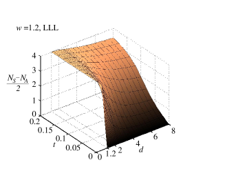
(c) (d)

Figure 3: (Color online) $(N_{S}-N_{A})/2$ (or $\langle(S_{z})_{SAS}\rangle$ when the Hamiltonian $\hat{H}$ is written in the SAS-basis) as a function of layer separation $d$ and tunneling amplitude $t$ for $\nu=1/2$ and $N=8$ electrons for single-layer width (a) $w=0$, (b) $w=0.6$, (c) $w=1.2$ and $w=2.4$.

We know from earlier work Peterson et al. (2008b, a) that finite layer width within a single quantum well, at least in the large tunneling and small layer separation limit, i.e., the one-component limit, may enhance the overlap between $\Psi_{0}$ and $\Psi_{\mathrm{Pf}}$. In Fig. 2(a) and (b) we show $\langle\Psi_{0}|\Psi_{331}\rangle$ and $\langle\Psi_{0}|\Psi_{\mathrm{Pf}}\rangle$, respectively, versus layer separation $d$ and single layer width $w$ for small tunneling $t=0$ and large tunneling $t=0.2$. For the small tunneling situation where 331 is a good ansatz, we see clearly that for $w=0$ the overlap is maximum for a finite value of $d\sim 2$. However, for finite $w$ we find that the position of maximum overlap does not change much and, in fact, for large $w$ the maximum overlap obtains essentially for the $w\gtrsim d$ condition.

In the case of $\Psi_{\mathrm{Pf}}$ (Fig. 2(b)) we find a result similar to the single- layer finite-thickness results (cf. Ref. Peterson et al., 2008a) where the overlap with the exact state is nearly constant for increasing $w$ and $d$. For $w=d$ we expect this behavior but it is interesting to note how robust the overlap is for finite $w$ and large $d$.

In Fig. 1(b)-(d) we consider the overlap between the exact state and the 331 and Pf states as function of separation and tunneling for finite layer widths of $w=0.6$, 1.2, and 2.4. If we consider first $\langle\Psi_{0}|\Psi_{\mathrm{Pf}}\rangle$ we see that not much changes for different values of $w$ as one would expect from examining Fig. 2(b). The only real qualitative change is that for $w=d$ for $w=0.6$ and 2.4 the overlap is non-zero, albeit very small, compared to the $w=0$ case where it is identically zero. However, for $w=1.2=d$ the overlap is zero, thus, we suppose that the small but non-zero overlap for $d=w$ is simply a finite size effect. For the overlap between the exact state and the 331 variational state we find that finite single layer width has two effects. First, it slightly lowers the maximum overlap obtained (this is evident in Fig. 2) and reduces the area in $d$-$t$ phase space where the 331 state is a good ansatz. In essence, for finite $w$ the Pfaffian phase pushes out the 331 phase, at least as far as wavefunction overlap determines the phase.

IV.2 Is the system one- or two-component?–lowest Landau level

Due to the potential confusion between whether the pseudo-spin operator $(\hat{S}_{z})_{SAS}$ or $(\hat{S}_{x})_{\mathrm{layer}}$ controls the tunneling we will report our results in terms of $(N_{S}-N_{A})/2$ where $N_{S}$ and $N_{A}$ are the expectation values of the total number of particles in the symmetric $S$ or antisymmetric $A$ state, respectively. This is the more precise variable since whether we are calculating $(\hat{S}_{z})_{SAS}$ or $(\hat{S}_{x})_{\mathrm{layer}}$ the answer is always equal to $(N_{S}-N_{A})/2$.

Our conclusion so far, based on overlap calculations, is completely consistent with the calculated expectation value of $(N_{S}-N_{A})/2$ which is essentially the order parameter describing the one-component to two-component transition, i.e., $(N_{S}-N_{A})/2\approx N/2$ describes a one-component phase since in that case $N=N_{S}$, whereas $(N_{S}-N_{A})/2\approx 0$ describes a two-component phase since in that case $N_{S}=N_{A}=N/2$. Note that in our $N=8$ system the maximum and minimum value of the pseudo-spin expectation value is 4 and 0, respectively. Fig. 3(a)-(d) shows the calculated $(N_{S}-N_{A})/2$ as a function of $d$ and $t$ for $w=0$, $w=0.6$, $w=1.2$, and $w=2.4$ . First we consider $w=0$ (Fig. 3(a)). For $d=0$ and $t=0$ the system is two-component and the system is SU(2) symmetric. Only a small amount of tunneling is required to very quickly push the system to be one-component. As $d$ is increased, more tunneling is required to make the system one-component. Of course, this can be readily understood physically: for non-zero layer separation $d$ the electrons in the symmetric state pay a higher Coulomb energy price than electrons in the antisymmetric state since $1/r>1/\sqrt{r^{2}+d^{2}}$, for $d\neq 0$.

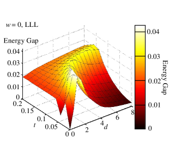
(a) (b)

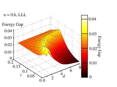
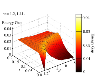
(c) (d)

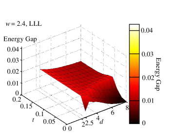
Figure 4: (Color online) FQHE energy gap as a function of layer separation $d$ and tunneling amplitude $t$ for the $\nu=1/2$ lowest LL system with $N=8$ electrons. We consider single quantum well widths of (a) $w=0$, (b) $w=0.6$, (c) $w=1.2$, and (d) $w=2.4$. The energy gap is also color-coded such that black is zero gap and white is maximum on a scale from zero to 0.0425 in Coulomb energy units, $e^{2}/(\kappa l)$.

For non-zero single-layer width (finite $w$) the general behavior outlined above does not change appreciably, cf. Figs. 3(b)-(d). The only real difference is that for increasing $w$, less tunneling is required, at the same value of layer separation $d$, to make the system one-component. That is, it is easier to push the system into one-component behavior via tunneling when $w\neq 0$.

Comparing these results to our overlap results shown in Fig. 1 we see that when the system is effectively two-component for weak tunneling the Halperin 331 state has a higher overlap with the exact state than the Moore-Read Pfaffian state. This is expected since the Pf state describes a one-component state. On the other hand, when the system is effectively one-component for strong tunneling the one-component Pf state has a higher overlap with the exact state $\Psi_{0}$ than $\Psi_{331}$ does. Looking closer, one finds that when $(N_{S}-N_{A})/2$ is increased from zero towards $(N_{S}-N_{A})/2\sim 2.5$ the overlap with the exact state switches from being higher with the two-component 331 state to the one-component Pf state (this is true irrespective of $w$). In other words, the two-component description of the exact state provided by $\Psi_{331}$ survives until nearly 60$\%$ more electrons are in the symmetric state than the antisymmetric state–the two-component 331 state is surprisingly robust to tunneling that drives the system towards one-component behavior.

IV.3 Will the system display the FQHE?–lowest Landau level

Wavefunction overlap and pseudo-spin are only two properties that elucidate the physics. Another property is the energy gap above the $L=0$ ground state in the excitation spectra; a crucial characteristic that determines the incompressibility or the robustness of the FQHE. In Fig. 4(a)-(d) we show the energy gap, defined as the difference between the first excited and ground state energies at constant $N_{\phi}$, as a function of $d$ and $t$ for the $\nu=1/2$ lowest LL system for (a) $w=0$, (b) $w=0.6$, (c) $w=1.2$, and (d) $w=2.4$. It is clear that for finite $d$ and $t$ there is a 1/2 FQHE with a finite gap. At the SU(2) symmetric point the energy gap is vanishingly small. Interestingly, the energy gap has a peak in $t$-$d$ space–a ridge along which the energy gap is maximum. Generally, as $w$ is increased the value of the energy gap decreases as is expected since finite width of a single quantum well reduces the Coulomb energy by softening it. For $w=2.4$, the maximum width considered, the energy gap retains the basic qualitative structure as for the other widths, however, its overall value is very small. Note as well that the maximum energy gap ridge is approximately located at the point in the $d$-$t$ parameter space where the overlap between the exact state crosses over from being larger with the Pfaffian ansatz and the 331 ansatz (more on this below), i.e., the gap is maximum close to the transition line between 331 and Pfaffian.

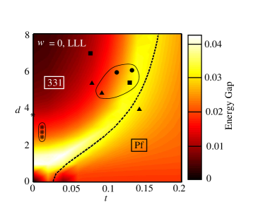
(a) (b)

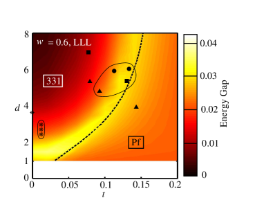
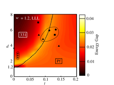
(c) (d)

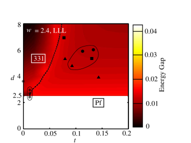
Figure 5: (color online) Quantum phase diagram (QPD) and FQHE gap (color coded) versus layer separation $d$ and tunneling strength $t$ for widths (a) $w=0$, (b) $w=0.6$, (c) $w=1.2$, and (d) $w=2.4$. For the QPD, the 331 and Pf phases (as discussed in the text) are separated by a dashed black line and labeled appropriately. The FQHE gap is given as a contour plot with color coding given by the color-bar from dark to light, i.e., white being a largest value of 0.0425 and black being value of 0. The asterisks, triangles, circles, and squares correspond to the different experiments in Refs. Eisenstein et al., 1992, Suen et al., 1992a, Suen et al., 1994, Shabani et al., 2009a and Luhman et al., 2008, respectively. Only experimental points showing FQHE are within the large solid circles in (a) with the lower smaller circles and upper larger circles indicating experiments in double-quantum-well structures and WQW structures, respectively. We note that the single triangle on the Pf side of the QPD does not manifest any experimental FQHE indicating that the theoretical gap may be overestimated for the Pf state.

In Fig. 5 we project the energy gap onto the two-dimensional $t$-$d$ plane with the color coding indicating the numerical FQHE gap strength on the same scale as in Fig. 4. Note that the Coulomb interaction is undefined for $d<w$ so no results are obtained in that case. On this same plot we draw with a black dashed line the line that separates the 331 phase from the Pfaffian phase. This phase boundary is determined by noting which state has a higher overlap with the exact state $\Psi_{0}$ in which region of parameter space, i.e., if $\langle\Psi_{331}|\Psi_{0}\rangle$ is larger than $\langle\Psi_{\mathrm{Pf}}|\Psi_{0}\rangle$ then we say the exact system is in the 331 phase and vice-versa. Note that the dashed line is only an operational phase boundary within our calculation since all we know is that the 331 (Pf) has higher (lower) overlap above (below) this line. We cannot rule out the possibility that the in thermodynamic limit some other state (including possibly a compressible state) besides the $\Psi_{331}$ or $\Psi_{\mathrm{Pf}}$ dominates.

We show the approximate quantum phase diagram (QPD) for all four values of the layer width parameter (a) $w=0$, (b) $w=0.6$, (c) $w=1.2$, and (d) $w=2.4$. The zero- (Fig. 5(a)) and the intermediate-width (Fig. 5(b)) results are of physical relevance whereas the (unrealistically) large width results (Fig. 5(c) and (d)) are provided here only for completeness (since this is the regime where the Pf state dominates over the 331 state in the quantum phase diagram). We note that we are using the simplistic Zhang-Das Sarma (ZDS) model Zhang and Das Sarma (1986) for describing the well width effect, and crudely speaking $w=1$ in the ZDS model corresponds roughly to $w_{QW}\approx 6$ where $w_{QW}$ is the corresponding physical (i.e., effective single-layer) quantum well width. For a single WQW, where the effective bilayer is created by the self-consistent potential of the electrons themselves Luhman et al. (2008); Shabani et al. (2009a); Suen et al. (1992a, 1994), our $w$ is typically much less than the total width $W$ of the WQW–very roughly speaking $w\sim W/12$, and $d\sim W/2$. As emphasized above, we treat $t$, $d$, and $w(<d)$ as independent tuning parameters.

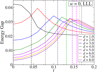
(a) (b)

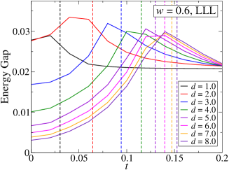
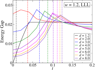
(c) (d)

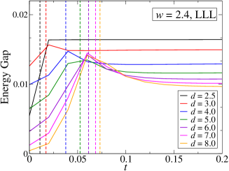
Figure 6: (color online) FQHE energy gap versus tunneling strength $t$ for several values of layer separation $d$ for (a) $w=0$, (b) $w=0.6$, (c) $w=1.2$, and (d) $w=2.4$. A dashed vertical line of the same color corresponds to the boundary between the Pfaffian phase (right of the line) and the 331 phase (left of the line).

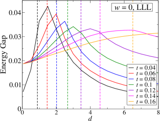
(a) (b)

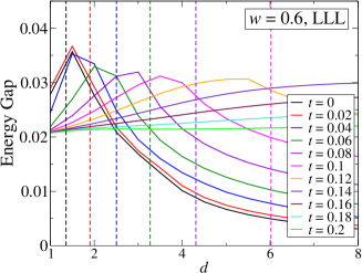
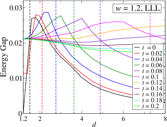
(c) (d)

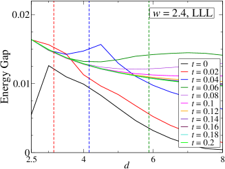
Figure 7: (color online) FQHE energy gap versus layer separation $d$ for a few values of tunneling strength $t$ for (a) $w=0$, (b) $w=0.6$, (c) $w=1.2$, and (d) $w=2.4$. A dashed vertical corresponds to the phase boundary between the Pfaffian phase (left of the line) and the 331 phase (right of the line).

In Fig. 5, we have put as discrete symbols all existing $\nu=1/2$ bilayer published FQHE experimental data (both for double quantum well systems and single wide-quantum-wells) in the literature, extracting the relevant parameter values (i.e., $d$ and $t$) from the experimental works Eisenstein et al. (1992); Suen et al. (1992a, 1994); Luhman et al. (2008); Shabani et al. (2009a). Because of the ambiguity and uncertainty in the definition of $w$ (i.e., how to precisely relate our theoretical $w$ in the Zhang-Das Sarma model to the experimental layer width in real samples), we have put the data points on all four QPDs shown in Fig. 5 although the actual experimental width values correspond to only Figs. 5(a) and (b). See Sec. VIII for a detailed description of exactly how the experimental points were determined.

Results shown in Fig. 5 bring out several important points of physics not clearly appreciated earlier in spite of a great deal of theoretical exact diagonalization work on $\nu=1/2$ bilayer FQHE:
(i) It is obvious that large, or small, $t$ and small, or large, $d$, in general, lead to a decisive preference for the existence of $\nu=1/2$ Pf, or 331, FQHE. The fact that large $t$ values would preferentially lead to the Pf state over the 331 state is, of course, expected since the system becomes an effective one-component system for large tunneling strength.
(ii) What is, however, not obvious, but apparent from the QPDs shown in Fig. 5, is that the FQHE gap (given in color coding in the figures) is maximum near the phase boundary between 331 and Pf.
(iii) Another non-obvious result is the persistence of the 331 state for very large (essentially arbitrarily large!) values of the tunneling strength $t$ as long as the layer separation $d$ is also large–thus having a large $t$ by itself, as achieved in the Luhman et al. experiment Luhman et al. (2008), is not enough to realize the single-layer $\nu=1/2$ Pf FQHE, one must also have a relatively small value of layer separation $d$ so that one is below the phase boundary (dashed line) in Fig. 5. The explanation for the Luhman experimental $\nu=1/2$ FQHE being a 331 sate, as can be seen in Fig. 5, is indeed the fact that both $t$ and $d$ are large in these samples making 331 a good variational state.
(iv) An important aspect of Fig. 5 is that the Pf FQHE gap tends to be very small–this is particularly true for larger values of $w$, where the Pf overlap is large. This implies, as emphasized by Storni et al. Storni et al. (2008), that the observation of a $\nu=1/2$ Pf state is unlikely since the activation gap would be extremely (perhaps even vanishingly) small.
(v) For larger values of $w$ (and large $t$), our calculated QPD is dominated by the Pf state–particularly for the unrealistically large width $w=2.4$ (corresponding to $w_{QW}\sim 14$!) where all the experimental $d$ and $t$ values fall in the Pf regime of the phase diagram. We emphasize, however, that this Pf-dominated large-$w$ (and large-$t$) regime will be difficult to access experimentally since the FQHE gap would be likely extremely small as in Fig. 5. Our results however cannot decisively rule out the possibility of a $\nu=1/2$ Pfaffian state in the strong tunneling and small separation regime.

We now discuss the published experimental results in light of our theoretical QPD. First, we note that most of the existing experimental points fall on the 331 side of the phase diagram which is consistent with our QPD in Fig. 5. In particular, only samples on the 331 side of the QPD with reasonably large FQH gaps, i.e., the data points close to the phase boundary, exhibit experimental FQHE. By contrast, the one data point (solid triangle in Figs. 5(a) and (b)) on the Pf side of the phase boundary does not manifest any observable FQHE in spite of its location being in a regime of reasonable FQHE excitation gap according to our phase diagram. This is consistent with the finding of Storni et al. Storni et al. (2008) that the $\nu=1/2$ FQHE gap in a single-layer system is likely to be vanishingly small in the thermodynamic limit. It is, therefore, possible that the Pf regime in our QPD has a much smaller excitation gap than what we obtain on the basis of our $N=8$ particle diagonalization calculation. We refer to Storni et al. Storni et al. (2008) for more details on the theoretical status of the single-layer LLL $\nu=1/2$ FQHE.

For a more detailed view of the $\nu=1/2$ bilayer FQHE, we show in Figs. 6(a)-(d) and 7(a)-(d), respectively, our calculated FQHE gap as a function of $t$ (for a few fixed $d$ values) and as a function of $d$ (for a few fixed $t$ values). Note that similar results were obtained by Nomura and Yoshioka in Ref. Nomura and Yoshioka, 2004, however, they only considered the energy gap versus tunneling for two values of separation $d$ and fixed $w=3.8$ for a $N=6$ electron system, which is aliased with a possible FQHE at $\nu=2/3$ and therefore suspect. In each figure, we also depict the line separating the 331 (smaller $t$/larger $d$) and the Pf (larger $t$/smaller $d$) regimes in the phase diagram. The qualitatively interesting point is, of course, the non-monotonicity in the FQHE gap as a function of $t$ or $d$ with a maximum close (but always on the 331 side) to the phase boundary. The non-monotonicity in the FQHE gap as a function of $t$ (but not $d$) was earlier pointed out, but our finding that the peak lies always on the 331 side of the phase boundary is a new result. We emphasize that this result is strong evidence that the 331 phase is the dominant FQHE phase in $\nu=1/2$ systems. We believe that the only chance of observing the $\nu=1/2$ Pf FQHE is to look on the Pf side of the phase boundary at fairly large values of $d$ and $t$. This is in sharp contrast to the SLL $\nu=5/2$ bilayer FQHE where we show in Section V that there are two sharp ridges far away from each other in the $d$-$t$ space corresponding to the $\nu=5/2$ Pf and 331 bilayer phases Peterson and Sarma (2009).

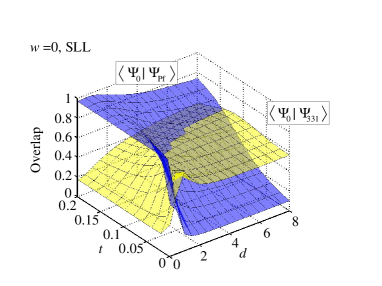
(a) (b)

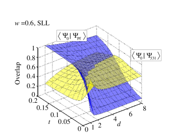
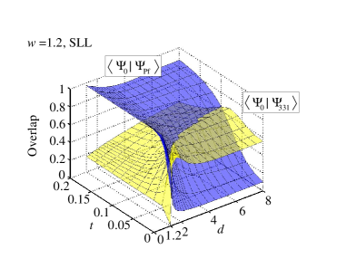
(c) (d)

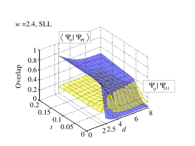
Figure 8: (Color online) Wavefunction overlap between the exact ground state $\Psi_{0}$ and the Pf state $\Psi_{\mathrm{Pf}}$ (blue (dark gray)) and 331 state $\Psi_{331}$ (yellow (light gray)) as a function of distance $d$ and tunneling amplitude $t$ for the half-filled second LL with $N=8$ electrons and width (a) $w=0$, (b) $w=0.6$, (c) $w=1.2$, and (d) $w=2.4$ ($d>w$ necessarily).

We conclude this section by commenting on the nature of the quantum phase transition (QPT) between the 331 and the Pf phase in the $d$-$t$ space. Our calculated QPD implies a continuous QPT from the strong-pairing 331 to the weak-pairing Pf state with increasing $t$ and/or decreasing $d$ as predicted by Read and Green Read and Green (2000). (Note this has also been very recently discussed by Dimov, Halperin, and Nayak Dimov et al. (2008).) In fact, our finite size diagonalization based QPD of Fig. 5 is topologically equivalent to the phase diagram predicted by Read and Green (Fig. 1 of Ref. Read and Green, 2000). We emphasize, however, that we cannot distinguish a quantum phase transition from a crossover because of the limitations of finite size calculations. It is also possible that a different phase, e.g. a compressible composite fermion Fermi liquid phase, has lower energy and intervenes between the 331 and Pf phases so that the system goes from 331 to Pf (or vice versa) through two first-order transitions. What we have shown here is that if the $\nu=1/2$ bilayer Pf phase exists at all, it would manifest most strongly in very wide samples and close to the phase boundary with the 331 phase with an extremely small FQHE excitation gap. We have also shown, through an explicit comparison with our $t$-$d$-$w$ phase diagram (Fig. 5) that all published $\nu=1/2$ FQHE data Luhman et al. (2008); Shabani et al. (2009a); Suen et al. (1992a, 1994); Eisenstein et al. (1992) are consistent with the existence of only the 331 phase in the LLL. Our work does not rule out the possibility of a weak Pf FQHE at $\nu=1/2$ for large values of tunneling.

V Second Landau Level

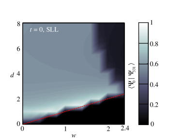
(a) (b)

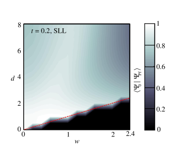
Figure 9: (Color online) Wavefunction overlap between the exact ground state $\Psi_{0}$ and $\Psi_{\mathrm{Pf}}$ at strong tunneling $t=0.2$ (a) and $\Psi_{331}$ at zero tunneling $t=0$ (b) as a function of separation $d$ and single-layer well width $w$ (where $d\geq w$) for the SLL with $N=8$ electrons. White corresponds to an overlap of unity while black corresponds to an overlap of zero. As in Fig. 2, the dashed red line is the condition $w=d$ and for $w>d$ the bilayer system is undefined, i.e., the single-layer width cannot be larger than the layer separation.

We now consider the same set of questions we asked regarding the physics of FQHE bilayers in the $\nu=1/2$ lowest LL (Sec. IV) about the bilayer FQHE systems in the second Landau level (SLL). Our approach here is to theoretically consider a single-layer FQHE at a half-filled SLL system, i.e., $\nu=2+1/2=5/2$ where the first two lowest Landau levels of spin-up and spin-down are completely occupied and inert. Thus, the half-filled SLL interacting electrons are projected into the LLL using the appropriate SLL Haldane pseudopotentials Haldane (1983). The exact nature of this procedure has been given many times in many places in great detail and will not be reiterated here (see Ref. Jain, 2007 for a good description). To consider a SLL bilayer system we then allow the single-layer to become a bilayer by reducing the tunneling and/or increasing the layer separation $d$. There are actually quite subtle points in defining this procedure in the SLL and they are discussed below in Sec. V.4 in detail. However, our procedure is completely well defined theoretically, and is a direct analog of the $\nu=1/2$ LL calculation in the SLL.

V.1 What is the physics?–second Landau level

(a) (b)

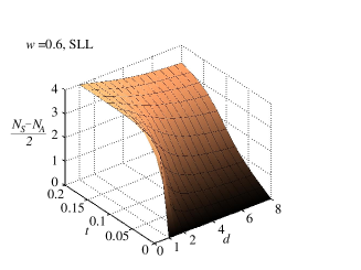
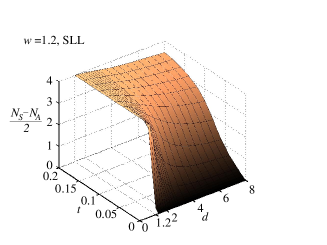
(c) (d)

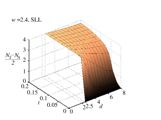
Figure 10: (Color online) $(N_{S}-N_{A})/2$ as a function of distance $d$ and tunneling amplitude $t$ for the half-filled second Landau level, $N=8$ electrons, and (a) $w=0$, (b) $w=0.6$, (c) $w=1.2$, and (d) $w=2.4$.

The calculated wavefunction overlap between the exact ground state $\Psi_{0}$ and the two appropriate candidate variational wavefunctions ($\Psi_{\mathrm{Pf}}$ and $\Psi_{331}$) as a function of distance $d$ and tunneling energy $t$ is shown in Fig. 8 for single-layer widths of $w=0$, $w=0.6$, $w=1.2$, and $w=2.4$. First we focus on the situation with zero width $w=0$ (Fig. 8(a)) and concentrate on the overlap with $\Psi_{\mathrm{Pf}}$. In the limit of zero tunneling and zero $d$ the overlap with $\Psi_{\mathrm{Pf}}$ is small–approximately 0.5 (unclear from the figure). However, only weak tunneling is required to produce a state with a sizable overlap of approximately $\sim 0.96$ and as tunneling increases this overlap remains large and approximately constant. For $d\neq 0$, in the weak tunneling limit, the overlap with $\Psi_{\mathrm{Pf}}$ decreases drastically. Adding moderate to strong tunneling we obtain a sizable overlap, decreasing gently in the large $d$ limit. This shows that the strong-tunneling (one-component) regime is well described by the Pf state. This strong tunneling Pf regime appears to be robust.

Next we consider the overlap between $\Psi_{0}$ and $\Psi_{331}$. In the zero tunneling limit, as a function of $d$, the overlap starts small, increases to a moderate maximum of $\approx 0.80$ at $d\sim 1$ before achieving an essentially constant value of $\approx 0.56$. For $d>4$ the overlap remains relatively constant and slowly decreases as the tunneling is increased (in fact, there is a slight increase in the overlap to $\sim 0.6$ for a region of positive $d>4$ and $0.1\lesssim t\lesssim 0.15$). Thus, the weak-tunneling (two-component) regime is well described by $\Psi_{331}$.

Similar to what we did in the LLL, we consider the effects of finite width, knowing that it may enhance the overlap Peterson et al. (2008b, a). In Fig. 9 (a) and (b) we show $\langle\Psi_{0}|\Psi_{331}\rangle$ and $\langle\Psi_{0}|\Psi_{\mathrm{Pf}}\rangle$, respectively, versus layer separation $d$ and single layer width $w$ for small tunneling $t=0$ and large tunneling $t=0.2$. In the zero tunneling limit (Fig. 9(a)) we see that the overlap can be increased significantly ($\sim 0.94$) by using $d\approx 1$ and $w\approx d$. The overlap between the exact state and the 331 state remains high with increasing width as long as the layer separation $d\approx 1$–this compares with the LLL case where the overlap is maximum for a larger separation near 1.8. However, the general feature that the maximum does not change appreciably with increasing $w$ is consistent with the LLL results. The main difference is the overlap with 331 is lower, and increasing $w$ and $d$ eventually pushes the overlap to zero.

For the strong tunneling limit ($t=0.2$), in the case of $\Psi_{\mathrm{Pf}}$ (Fig. 2(b)), our results are consistent with the single- layer finite-thickness results (cf. Refs. Peterson et al., 2008b and Peterson et al., 2008a). Compared to the LLL, however, the overlap increases to a maximum for a finite $w$ and that behavior continues to hold when $d$ is increased. Eventually, large single-layer width causes the overlap with the Pfaffian state to decrease for any $d$ significantly larger than $w$. Thus, finite layer width enhances the overlap with both 331 and Pf states in their regimes of phase space.

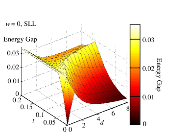
(a) (b)

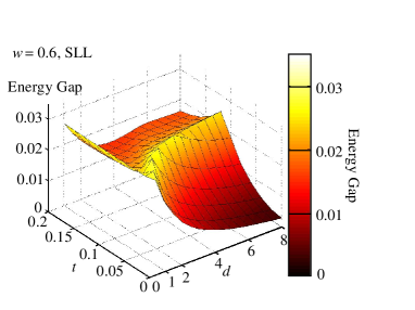
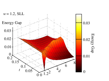
(c) (d)

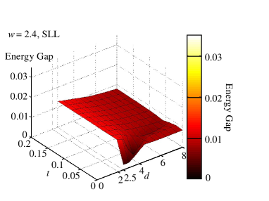
Figure 11: (Color online) FQHE energy gap as a function of layer separation $d$ and tunneling amplitude $t$ for the second LL system with $N=8$ electrons. We consider single quantum well widths of (a) $w=0$, (b) $w=0.6$, (c) $w=1.2$, and (d) $w=2.4$. The energy gap is also color-coded such that black is zero gap and white is maximum on a scale from zero to 0.035.

By examining Fig. 8(b)-(d) we see results qualitatively similar to the LLL results shown in Fig. 1. The real difference here is that the overlap between the exact state and the Pf state, in the region of phase space where it is better than the 331 state, is higher in the SLL than it is in the LLL. This is expected behavior when one considers the single-layer results Peterson et al. (2008b, a) where the Pf is known to be an excellent candidate for the $\nu=5/2$ single-layer FQHE. The other difference complimentary to the Pfaffian behavior is that the overlap between the exact state and the 331 state is lower in the SLL than it is in the LLL. In fact, for large layer width $w=2.4$ (Fig. 8(d)) the overlap with the 331 is quite low and it would be unreasonable to assume that the exact state is adequately described by the Halperin 331 state. The Pfaffian overlap is also lower for $w=2.4$ in the SLL than it is in the LLL (somewhat surprisingly). In fact, after investigating the FQHE energy gap for $w=2.4$ (below in Sec. V.3) it is clear that the bilayer SLL system most likely would not exhibit any FQHE for such large widths. Again, similar to the LLL results (Fig. 1(b)-(d)), we note that for increasing $w$, the region in phase space described by the Pf phase increases at the expense of the 331 state.

V.2 Is the system one- or two-component?–second Landau level

Fig. 10 shows the calculated value of $(N_{S}-N_{A})/2$ as a function of $d$ and $t$ with (a) $w=0$, (b) $w=0.6$, (c) $w=1.2$, and $w=2.4$ and, as before, our overlap based conclusions are consistent with the value of $(N_{S}-N_{A})/2$. It is difficult to clearly tell the difference between the results in the SLL compared to those in the LLL. The slight difference between the two is that in the large $d$ limit slightly more tunneling is required to drive the system to the one-component regime than in the LLL case. Further, in the strong tunneling limit, the SLL system’s one-component character is more robust to increasing layer separation $d$–but only just. Again, similar to the LLL, we find that when $(N_{S}-N_{A})/2\sim 2.5$ the overlap with the exact ground state switches from being either higher with the Pf state or the 331 state.

V.3 Will the system display the FQHE?–second Landau level

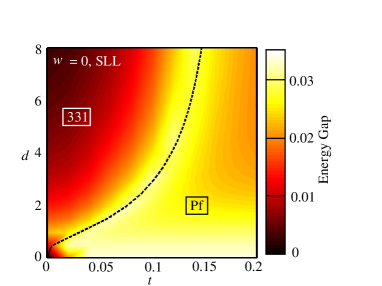
(a) (b)

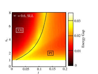
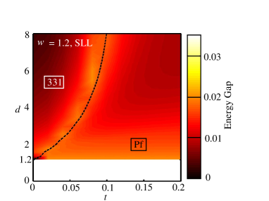
(c) (d)

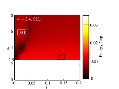
Figure 12: (color online) Quantum phase diagram (QPD) and FQHE gap (color coded) for the second LL for widths (a) $w=0$, (b) $w=0.6$, (c) $w=1.2$, and (d) $w=2.4$. For the QPD, the 331 and Pf phases are labeled appropriately and the gap is given as a contour plot with color coding given by the color-bar from dark to light, i.e., white being a largest value of 0.035 and black being value of 0.

In Fig. 11(a)-(d) we show the FQHE energy gap as a function of $d$ and $t$ for the SLL system for (a) $w=0$, (b) $w=0.6$, (c) $w=1.2$, and (d) $w=2.4$. Similar to the LLL, it clear that for finite $d$ and $t$, a 5/2 FQHE with a finite gap (being either 331 or Pf) exists in a realistic parameter regime. There is a clear qualitative difference between the lowest and second LLs, however. In the SLL, the largest FQHE energy gap is obtained in the zero $d$ limit for finite tunneling. That is, in the region where the Moore-Read Pfaffian ansatz is the better description of the exact ground state, the energy gap is largest. With an energy gap nearly as large is the “ridge” region identified in our LLL results–again the ridge lies in the region of $d$-$t$ phase space corresponding to the “quantum phase transition” between the Pf phase and 331 phase. Finite single-layer width $w$ (Fig. 11(b)-(d)) decreases the overall energy gap and moves the ridge area to weaker tunneling. Note that for the largest width considered ($w=2.4$) the energy gap is very small and the ridge has essentially become a “valley” and the overall energy gap is very small.

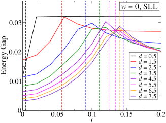
(a) (b)

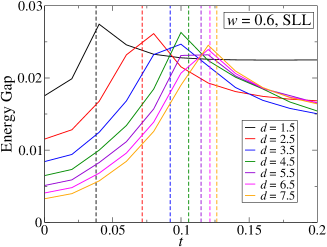
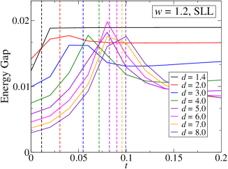
(c) (d)

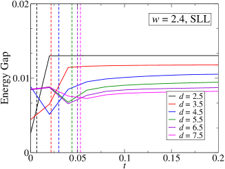
Figure 13: (color online) FQHE energy gap versus tunneling strength $t$ for a few values of layer separation $d$ for (a) $w=0$, (b) $w=0.6$, (c) $w=1.2$, and (d) $w=2.4$. A dashed vertical line of the same color corresponds to the boundary between the Pfaffian phase (right of the line) and the 331 phase (left of the line).

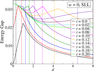
(a) (b)

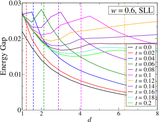
(c) (d)

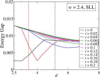
Figure 14: (color online) FQHE energy gap versus layer separation $d$ for a few values of tunneling strength $t$ for (a) $w=0$, (b) $w=0.6$, (c) $w=1.2$, and (d) $w=2.4$. A dashed vertical line of the same color corresponds to the boundary between the Pfaffian phase (left of the line) and the 331 phase (right of the line).

We now discuss the approximate quantum phase diagram for the bilayer system for the SLL as shown in Fig. 12 for single-layer widths (a) $w=0$, (b) $w=0.6$, (c) $w=1.2$, and (d) $w=2.4$. This QPD is calculated the same way as it is for the LLL (cf. Fig. 5)– identifying the 331 and Pf phases as the regions in the parameter space where the overlap with $\Psi_{0}$ is larger (Fig. 8). In general, the two-component 331 phase (the upper left region) has a weaker SLL FQHE than that of the one-component Pf (the lower right region). Figure 12, which is an important prediction of our work, shows that in the SLL bilayer system, both the 331 and Pf states should be visible, and in a realistic finite thickness system (Fig. 12(b) and (c)), the FQHE gap would become very small, perhaps even zero, in between the two phases.

Again, we ask the natural question whether our numerically obtained transition from the large-$d$ (small-$t$) region to the small-$d$ (large-$t$) region is a quantum phase transition or a crossover. Of course a finite-size numerical study cannot definitively answer this question. Our results, however, are consistent with the findings Read and Green (2000) of Read and Green, and we believe that there would be a QPT between 331 and Pf phases in the second LL since a crossover between topologically trivial (331) and non-trivial (Pf) phases is difficult to contemplate. We also note that for the $w=0$ case, the quantum phase transition line seems to terminate at $d=0=t$ for the SLL and for $d=0$ and finite tunneling $t$ in the LLL, i.e., some finite $t$ is required to push the system into the Pf phase. Thus, our SLL results are more similar to the QPD of Read and Green Read and Green (2000) where a multi-critical point exists separating the 331 Abelian phase from the non-Abelian Pf phase when $t=0$. It is perhaps understandable that our SLL results would more closely resemble that of Read and Green since they were modeling a 1/2-filled bilayer FQHE state as $p_{x}+ip_{y}$ superconductor of composite fermions which is thought to be the appropriate description for the 1/2-filled FQHE in the SLL, not necessarily in the LLL. Further, in our SLL QPD, the Pf phase is quite strong–as indicated by the FQHE energy gap–along the $d=0$ and finite $t$ line, whereas in the LLL, the gap is quite small along that line. Of course, the parameters in Read and Green’s analysis are not directly related to our parameters–they have a chemical potential $\mu$ in an effective pairing Hamiltonian while we have layer separation $d$. Furthermore, our model is SU(2) symmetric at the $d=0=t$ point while their model has explicitly broken SU(2). More work will be needed to understand completely the similarities of our approach and that of Read and Green definitively, but the fact that the topology of our numerically calculated phase diagram of Fig. 12 strongly resembles that of the phase diagram discussed by Read and Green is highly suggestive.

In Figs. 13(a)-(d) and 14(a)-(d) we provide a detailed view of the SLL FQHE bilayer system with the FQHE energy gap given as a function of tunneling energy $t$ for several values of the layer separation $d$ and the energy gap as a function of layer separation for several values of tunneling energy, respectively. The FQHE energy gap as a function of tunneling is similar qualitatively to the results in the LLL. Namely, the gap rises to a peak value and then falls off. Of course, for $w=2.4$ (Fig. 13(d)) the FQHE gap structure is different than all other cases, lowest or second LL, in that the peak has turned into a valley.

In Fig. 14 we find that the behavior of the FQHE energy gap as a function of layer separation $d$ for constant tunneling energy $t$ is qualitatively different from the behavior in the LLL. The difference is that in the SLL the largest value of the energy gap is for $d=0$ and for increasing $d$ the energy gap decreases slightly to a minimum (for $t>0.02$) and then rises again to a peak. For increasing tunneling energy, the peak becomes more rounded. This behavior is qualitatively different from the lowest LL in that there are two peaks in the energy gap versus $d$ at constant $t$ instead of one–note that for $w=0$ and $t\leq 0.02$ there is only a single peak not unlike the lowest LL results. For zero layer width ($w=0$), the phase boundary between the one-component Pfaffian phase (to the left of the boundary line) and two- component 331 phase (to the right of the boundary) is to the left of the single peak in the energy gap for $t\leq 0.02$, moves to slightly right of the second energy gap peak for $0.02<t<0.1$, and then finally moves back to being left of the second energy gap peak. For $w=0.6$ in Fig. 14(b) there are two energy gap peaks and the phase boundary is slightly to the right of the peak for $t<0.1$ for $w=0.6$. For $t>0.1$ the phase boundary moves to the left of the second peak. For $w=1.2$ in Fig. 14(c) (except for $t=0$) the phase boundary is always to the left of the second energy gap peak. Lastly, we show results for $w=2.4$ in Fig. 14(d) for sake of completeness but it is clear that this case is most likely not a FQHE for any parameter values other than for very small $d$ and large $t$.

V.4 Bilayer FQHE in higher Landau levels

(a)

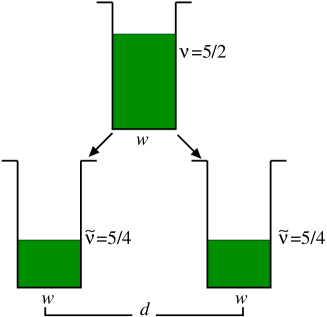
(b)

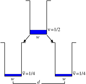
Figure 15: Schematic diagram depicting the FQHE system at total filling factor (a) $\nu=5/2$ and (b) $\nu=1/2$ being broken up into a bilayer system with each separate layer being at (a) $\tilde{\nu}=5/4$ and (b) $\tilde{\nu}=1/4$. The colored shaded section represents a density of electrons filling up a quantum well.

There is a conceptual difficulty that we postponed when discussing bilayer FQHE in the SLL which exists when discussing any bilayer FQHE in higher LLs. In fact, we carefully set up the initial SLL bilayer FQHE problem as starting with a single-layer, or one-component, system in the SLL (presumably the 1/2 filled SLL at $\nu=5/2$) and then systematically driving the system into a bilayer by the tuning of model parameters,. However, in our calculation, the electrons fractionally filling the SLL remain in the SLL throughout the procedure of tuning the system from one- to two-component. A bilayer FQHE at total filling factor $\nu=5/2$ would consist of two layers at single layer filling factor $\tilde{\nu}=(1/2)(5/2)=5/4$, see Fig. 15. This is compared to the LLL where the half-filled bilayer FQHE consists of $\nu=1/4+1/4=1/2$, i.e., two layers at $\tilde{\nu}=1/4$, which when combined yield total $\nu=1/2=2\tilde{\nu}$ (Fig. 15(b)).

The case of spin-less electrons (we consider the spin-full situation below) is depicted in Fig. 16. In the one-component limit, electrons in the half-filled SLL have total filling factor $\nu=1+1/2=3/2$–the LLL is completely filled and considered inert. In the two-component limit, when each of the two quantum well layers have been taken far apart from one another, the filling factor in each layer (assuming the electrons to have equal densities in each layer) will be $\tilde{\nu}=3/4$. Thus, the electrons in individual layers are in the lowest LL, not the SLL. The key conceptual difficulty is that we started with a one-component system at total $\nu=1/2$ in the second LL and ended up splitting it into a bilayer system of each layer at $\tilde{\nu}=3/4$ in the lowest LL, i.e., the electron LL index changed!

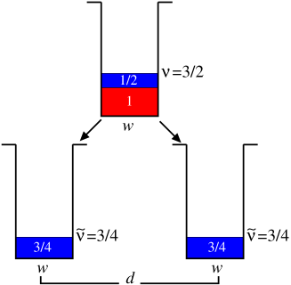
Figure 16: Schematic diagram depicting a spin-less FQHE system at total filling factor $\nu=3/2$ becoming a bilayer spin-less system with each layer at $\tilde{\nu}=3/4$. The fraction of the density fractionally filling a LL is colored blue (dark grey) while an inert LL (in this case the lowest) is colored red (light grey).

If one were to study bilayer FQHE in the SLL completely rigorously (necessarily numerically) one would have to consider–even for spin-less electrons–a system consisting of electrons with a layer degree of freedom (pseudo-spin) and at least two LL degrees of freedom. Furthermore, one would not necessarily be able to treat the electrons in the LLL (the 1 in the $1+1/2=3/2$) as inert. For the system we studied with $N=8$ electrons half-filling the second LL, one would need to fully consider $N=20$ interacting electrons with a layer degree of freedom and consider at least two LLs. Hence, the Hilbert space dimension would be extremely large–on the order of $10^{11}$ states. A Hilbert space dimension of $10^{11}$ is out of reach for any numerical procedure for any computer.

The experimental reality makes the situation more complicated due to the inclusion of spin. Half-filled FQHE in single-layer, presumably, one-component systems has only been observed in the SLL, i.e., $\nu=5/2$, which is modeled successfully by treating the completely filled spin-up and spin-down LLLs as inert. Once the system is made into a bilayer we are left with, in the extreme layer separation limit, two systems at $5/4=1+1/4$ filling. When the layers are very far apart (large $d$ and necessarily weak $t$) it would be expected that the structure of the 5/4 filled systems would be identical (since they would not interact) and the spin-up LLL would be filled and inert and the remaining electrons would fill the spin-down LLL up to 1/4 filling. Such a situation is depicted in Fig. 17(b). If, on the other hand, the system is barely becoming two-component, perhaps the simplest possibility is that the two $\tilde{\nu}=5/4$ layers will consist of a completely filled spin-up LLL in one layer and spin-down LL in the other layer (see Fig. 17(a)). However, when the two layers are close enough that they begin to interact with one another–even without any tunneling–the situation quickly becomes complicated (as discussed below). It is not clear if any of the electrons in a bilayer FQHE at total $\nu=5/2$ can be considered inert and one might need to consider an interacting electron system where the electrons carry spin, pseudo-spin, and two, or possibly three, LLs indices, making such a problem intractable.

(a)

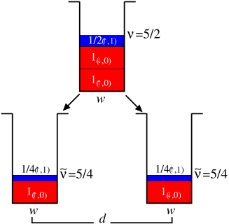
(b)

Figure 17: Schematic diagram depicting two possible scenarios for the spin-full FQHE system at total filling factor $\nu=5/2$ being broken up into a bilayer system with each separate layer being at $\tilde{\nu}=5/4$. In (a) we consider the small $d$ and strong $t$ limit where the lowest spin-up and spin-down Landau levels are completely occupied leaving a 1/4 filled spin-up Landau level in each layer. In (b) we depict the large $d$ and weak tunneling $t$ limit with the lowest spin-up LLL being filled in each layer leaving a 1/4-filled lowest Landau level of spin-down electrons in each layer. The notation is such that $\nu_{(\sigma,n)}$ corresponds to the filling factor $\nu$ for electrons with spin-$\sigma$ electrons with orbital Landau level index $n$, i.e., $1_{(\uparrow,0)}$ corresponds to filling factor 1 of spin-$\uparrow$ electrons with LLL index $0$.

We note that considering each layer to have $\tilde{\nu}=2+1/4$ filling so that, in analogy with the LLL bilayer situation, we have 1/4 filling in each SLL layer, does not resolve the ambiguity since this produces a total filling of $\nu=(2+1/4)+(2+1/4)=9/2$, taking us to the half-filled third orbital LL! Similarly, considering each layer to have $\nu=1+1/4$ filling leads to a total bilayer filling of $\nu=5/2$, but takes us from the LLL to the SLL in going from a one layer to a bilayer system. The conundrum here is not theoretical, but is about how one connects the theoretical results with the experimental bilayer 5/2 system. We emphasize that no such ambiguity arises for the $\nu=1/2=1/4+1/4$ bilayer system where all of the physics occurs in the LLL, both for individual layers and for the total bilayer. Also, there is no ambiguity in the strong tunneling regime where the bilayer effectively acts as a single layer system with $\nu=5/2$ as in a single 2D system.

For our fully spin-polarized model, however, there is an easy conceptual (and operational) way out of this ambiguity for the bilayer $\nu=5/2$ system. Since we assume the whole system (in both layers and in both orbital Landau levels) to have the same spin, the system is effectively spin-less (which is equivalent to assuming the Zeeman energy to be much larger than the cyclotron energy). In this spin-less (or spin-polarized) situation, each orbital LL by definition comes with just one spin index. Therefore, the $\nu=5/2$ balanced bilayer system is equivalent to a $\tilde{\nu}=(1/2)(5/2)=5/4=1+1/4$ filling in each layer, where the completely filled inert level in each layer is simply the LLL, and the 1/4-filled level in each layer is in the SLL. Since the LLL is inert, the incompressible FQH states form entirely in the SLL, and we can construct a Halperin 331 SLL state with $\nu=1/2$ from the two 1/4-filled SLL states in each individual layer in a manner similar to that for the $\nu=1/2$ LLL bilayer state. We emphasize that this simplicity is lost if we include both spin and layer indices on an equal footing since including the two spin indices (up and down) and two layer indices (right and left) lead to an immediate problem on how to assign individual $\tilde{\nu}$ values which, when combined into the total $\nu=2\tilde{\nu}$, lead to a bilayer SLL $\nu=5/2$ FQHE with both the total bilayer (i.e., $\nu$) and the individual layer (i.e., $\tilde{\nu}=\nu/2$) filling factor being in the SLL. (As emphasized already, the situation with two layers, two spins, and two orbital LLs is ambiguous unless the numerical diagonalization takes exactly into account the full dynamics of all three two-level quantum indices which is impossible to do for any computer.)

We mention that earlier theoretical work (alluded to above) by Zheng et al. Zheng et al. (1997), Das Sarma et al., Das Sarma et al. (1997, 1998), Demler et al. Demler and Das Sarma (1999), and Brey et al. Brey et al. (1999) did take into account the dynamical interplay between layer and spin indices with the conclusion that there should be a novel quantum canted antiferromagnetic phase in bilayers for situations where each individual layer state has a gap in the spectrum (e.g., $\nu=1+1$ or $1/3+1/3$ or $1+1/3+1+1/3$). For the case we are considering in the current work, i.e., $\nu=5/2$ and $\tilde{\nu}=\nu/2=5/4$, there is not necessarily a gap in the individual layer spectrum, and therefore a canted phase is not expected.

VI Conclusions

Our results concerning the $\nu=1/2$ LLL FQHE bilayer system point to strong evidence that the dominant FQH phase is the two-component Abelian Halperin 331 phase. We believe that the only chance of observing the $\nu=1/2$ non-Abelian Moore-Read Pfaffian FQHE is to look on the Pf side of the phase boundary (Fig. 5) at fairly large values of $d$ and $t$. This contrasts the SLL bilayer situation where there are two sharp ridges far away from each other in the $d$-$t$ space corresponding to the Pf and 331 phases. We note that for unrealistically large single layer width $w$ the Pf phase dominates the 331 phase but the FQHE gap is extremely small. If the Pf phase exists at all, it would manifest most strongly in wide samples and close to the phase boundary with the 331 phase.

In addition, we predict the existence of both the two-component 331 Abelian (at intermediate to large $d$ and small $t$) and the one-component Pfaffian non-Abelian (at small $d$ and intermediate to large $t$) $\nu=5/2$ SLL FQHE phase in bilayer structures. The observation of these two topologically distinct phases, one (Pf) stabilized by large inter-layer tunneling and the other (331) stabilized by large inter-layer separation would be a spectacular verification of the theoretical expectation Read and Green (2000) that bilayer structures allow quantum phase transitions between topologically trivial and non-trivial paired even-denominator incompressible FQHE states. The direct experimental observation of our predicted “two distinct branches” of two strong SLL FQHE regimes in bilayer structures, as shown in Fig. 12(a)-(c), with the FQHE gap being largest along the two ridges in the phase diagram as $d$ and $t$ are varied, will be compelling evidence for the existence of the $\nu=5/2$ non-Abelian Pf state.

Note that for small $d$ and $t$, Pf and 331 phases are continuously connected, indicating the possible existence of a quantum phase transition. We cannot, of course, dismiss a crossover due to the limitations of finite size calculations, but it is difficult to contemplate how an Abelian and non-Abelian phase could continuously go into each other without a quantum phase transition.

Besides our exact diagonalization results for the bilayer $\nu=1/2$ and 5/2 FQHE, we have raised an important conceptual issue involving the existence of Halperin type bilayer FQHE states in higher (i.e., beyond the lowest) Landau levels. In particular, the fact that two well-separated distinct layers have individual filling factors $\nu/2$, which necessarily lie in a lower orbital LL, make it tricky to define a composite bilayer Halperin wavefunction for $\nu$ which is in a higher LL. (This problem obviously does not arise in the LLL.) It is conceivable that any theoretical study of bilayer FQHE states in higher LLs must necessarily include the full dynamics involving layer, orbital LL, and spin degrees of freedom. This is an almost impossible theoretical challenge, and we hope that our work will motivate experimental activity in bilayer structures at total filling factor 5/2 in order to explore the possible difference between the physics of bilayer $\nu=1/2$ and $\nu=5/2$ systems.

VII Acknowledgements

We acknowledge support from Microsoft Q and DARPA QuEST. We also thank Nick Read and Kentaro Nomura for helpful discussions, and Bert Halperin for asking a particularly probing question.

VIII Appendix: Identifying the Experimental Points in the $\nu=1/2$ Bilayer FQHE Quantum Phase Diagram

We briefly describe our procedure for identifying the experimental data points in our calculated $\nu=1/2$ bilayer FQHE quantum phase diagram (Fig. 5). In other words, we explain how we extracted the parameter values $t$ (tunneling energy), $d$ (layer separation), and $w$ (layer width) for each experimental sample point shown in Fig. 5.

The tunneling energy $t$ is connected directly to the symmetric-antisymmetric gap $\Delta_{SAS}=t$ in our model and therefore we simply use the quoted value of $t$ (or $\Delta_{SAS}$) from the relevant experimental paper. The layer separation $d$ appears in our interlayer Coulomb interaction as $V_{\mathrm{inter}}=e^{2}/(\kappa\sqrt{r^{2}+d^{2}})$. For a true bilayer system the definition of $d$ is obvious (the well-center to well-center distance between the two quantum wells), and we use that value for $d$ from the experimental publications (see Fig. 18(a)). For a wide single-well system, where the effective bilayer arises as a direct result of the self-consistent density profile in the system, we choose $d$ as the distance between the two peaks in the calculated carrier density profile for the corresponding wide well sample (see Fig. 18(b)). These self-consistent density profiles are given in each experimental paper for each sample we show in Fig. 5. This procedure is, of course, imperfect–for example, the density profiles could be different from the calculated zero-field local density approximation (LDA) results since the systems is in the strong field FQHE regime. We do not, however, believe that this is a serious issue since the 2D dynamics of the electrons leading to FQHE is separable from the calculated density profile in the $z$-direction transverse to the 2D plane. In any case, the value of $d$, as given by the calculated LDA density profile, is the best one can do.

(a)

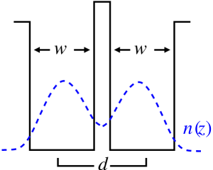
(b)

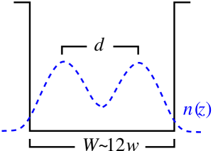
Figure 18: Schematic diagram depicting the two bilayer structures considered in this work. (a) shows a double quantum well structure along with a generic density profile in the $z$-direction $n(z)$ (blue dashed line) for experiments like Ref. Eisenstein et al., 1992 while (b) shows a single wide-quantum-well structure and generic density profile (blue dashed line) typical of experiments like Ref. Suen et al., 1992a.

Experiment	$d/l$	$t/(e^{2}/(\kappa l))$	$w/l$
Luhman et al., (squares), Ref. Luhman et al.,2008	5.3	0.13	0.4
	6.9	0.07	0.3
Eisenstein et al., (asterisks), Ref. Eisenstein et al.,1992	2.4	0.01	0.3
	2.7	0.01	0.3
	3.6	0.01	0.3
Suen et al., (triangles), Ref. Suen et al.,1992a, 1994	5.3	0.08	0.4
	4.8	0.09	0.4
	3.9	0.14	0.4
Shabani et al., (circles), Ref. Shabani et al.,2009a	5.9	0.11	0.25
	6.0	0.13	0.25

Table 1: Values of layer separation $d$, quantum well width $w$, and tunneling energy $t$ in units of magnetic length $l$ and Coulomb energy $e^{2}/(\kappa l)$, respectively, taken from Refs. Luhman et al., 2008,  Eisenstein et al., 1992, Suen et al., 1992a, Suen et al., 1994, and Shabani et al., 2009a as described in Section VIII.

The most problematic parameter for our model is the finite width parameter $w$ which, in the Zhang-Das Sarma model (Ref. Zhang and Das Sarma, 1986), does not correspond at all to the physical layer width. This is why we have shown the experimental points on all four “width” values in Fig. 5. It is known from earlier work He et al. (1990); Peterson et al. (2008a); Morf (1998); Morf et al. (2002); Ortalano et al. (1997); Park and Jain (1998); Park et al. (1999) that the Zhang-Das Sarma parameter $w$ has the following, very approximate, correspondence with the quantum well width parameter $w_{\mathrm{QW}}$: $w\simeq\frac{w_{\mathrm{QW}}}{6}$. Given that a balanced, symmetric, wide-quantum-well structure with a total width of $W$ has $w_{\mathrm{QW}}=W/2$ for each individual layer, we conclude $w_{\mathrm{ZDS}}\approx w_{\mathrm{QW}}/12$. This is, however, a very qualitative and crude estimate. Because of all the approximations involved in our depiction of the experimental data, points in Fig. 5 should be taken as a qualitative comparison, rather than a quantitative one.

In Table 1 we provide the values for $t$, $d$, and $w$ we get from individual experimental papers whose data points show up in Fig. 5

Lastly, we schematically show in Fig. 18 how $d$ and $w$ in our model correspond to those in the experimental sample. The tunneling energy $t$ corresponds directly to the symmetric-antisymmetric splitting, and the density profile in the wide well is obtained from LDA calculations for the experimental samples. Fig. 18(a) corresponds to double quantum well structure and typical density profile in the experiments by Eisenstein et al. Eisenstein et al. (1992) and Fig. 18(b) matches the single wide-quantum-well structure and typical density profile in experiments by Suen et al. Suen et al. (1992a, 1994), Luhman et al. Luhman et al. (2008), and Shabani et al. Shabani et al. (2009b).

References

- Luhman et al. (2008) D. R. Luhman, W. Pan, D. C. Tsui, L. N. Pfeiffer, K. W. Baldwin, and K. W. West, Physical Review Letters 101, 266804 (2008).
- Das Sarma et al. (2005) S. Das Sarma, M. Freedman, and C. Nayak, Phys. Rev. Lett. 94, 166802 (2005).
- Nayak et al. (2008) C. Nayak, S. H. Simon, A. Stern, M. Freedman, and S. D. Sarma, Rev. Mod. Phys. 80, 1083 (2008).
- Willett et al. (1987) R. Willett, J. P. Eisenstein, H. L. Störmer, D. C. Tsui, A. C. Gossard, and J. H. English, Phys. Rev. Lett. 59, 1776 (1987).
- Eisenstein et al. (1988) J. P. Eisenstein, R. Willett, H. L. Stormer, D. C. Tsui, A. C. Gossard, and J. H. English, Phys. Rev. Lett. 61, 997 (1988).
- Gammel et al. (1988) P. L. Gammel, D. J. Bishop, J. P. Eisenstein, J. H. English, A. C. Gossard, R. Ruel, and H. L. Stormer, Phys. Rev. B 38, 10128 (1988).
- Pan et al. (1999) W. Pan, J.-S. Xia, V. Shvarts, D. E. Adams, H. L. Stormer, D. C. Tsui, L. N. Pfeiffer, K. W. Baldwin, and K. W. West, Phys. Rev. Lett. 83, 3530 (1999).
- Eisenstein et al. (2002) J. P. Eisenstein, K. B. Cooper, L. N. Pfeiffer, and K. W. West, Phys. Rev. Lett. 88, 076801 (2002).
- Xia et al. (2004) J. S. Xia, W. Pan, C. L. Vicente, E. D. Adams, N. S. Sullivan, H. L. Stormer, D. C. Tsui, L. N. Pfeiffer, K. W. Baldwin, and K. W. West, Phys. Rev. Lett. 93, 176809 (2004).
- Csáthy et al. (2005) G. A. Csáthy, J. S. Xia, C. L. Vicente, E. D. Adams, N. S. Sullivan, H. L. Stormer, D. C. Tsui, L. N. Pfeiffer, and K. W. West, Phys. Rev. Lett. 94, 146801 (2005).
- Choi et al. (2008) H. C. Choi, W. Kang, S. Das Sarma, L. N. Pfeiffer, and K. W. West, Phys. Rev. B 77, 081301 (2008).
- Moore and Read (1991) G. Moore and N. Read, Nucl. Phys. B 360, 362 (1991).
- Dean et al. (2008) C. R. Dean, B. A. Piot, P. Hayden, S. D. Sarma, G. Gervais, L. N. Pfeiffer, and K. W. West, Phys. Rev. Lett. 100, 146803 (2008).
- foo (a) The 2 in comes from completely filling the lowest spin-up and spin-down Landau levels.
- He et al. (1991) S. He, X. C. Xie, S. Das Sarma, and F. C. Zhang, Phys. Rev. B 43, 9339 (1991).
- Greiter et al. (1992) M. Greiter, X. G. Wen, and F. Wilczek, Phys. Rev. B 46, 9586 (1992).
- He et al. (1993) S. He, S. Das Sarma, and X. C. Xie, Phys. Rev. B 47, 4394 (1993).
- Nomura and Yoshioka (2004) K. Nomura and D. Yoshioka, J. Phys. Soc. Jpn. 73, 2612 (2004).
- Shabani et al. (2009a) J. Shabani, T. Gokmen, and M. Shayegan, Phys. Rev. Lett. 103, 046805 (2009a).
- Halperin (1983) B. I. Halperin, Helv. Phys. Acta 56, 783 (1983).
- Read and Rezayi (1996) N. Read and E. Rezayi, Phys. Rev. B 54, 16864 (1996).
- Storni et al. (2008) M. Storni, R. H. Morf, and S. D. Sarma, Phys. Rev. Lett. 104, 076803 (2010).
- Papić et al. (2009) Z. Papić, G. Möller, M. V. Milovanović, N. Regnault, and M. O. Goerbig, Phys. Rev. B 79, 245325 (2009).
- Shabani et al. (2009b) J. Shabani, T. Gokmen, Y. T. Chiu, and M. Shayegan, Phys. Rev. Lett. 103, 256802 (2009b).
- Peterson et al. (2008a) M. R. Peterson, T. Jolicoeur, and S. D. Sarma, Phys. Rev. B 78, 155308 (2008a).
- Papić et al. (2009) Z. Papić, N. Regnault, and S. Das Sarma, Phys. Rev. B 80, 201303 (2009).
- Morf (1998) R. H. Morf, Phys. Rev. Lett. 80, 1505 (1998).
- Feiguin et al. (2009) A. E. Feiguin, E. Rezayi, K. Yang, C. Nayak, and S. Das Sarma, Phys. Rev. B 79, 115322 (2009).
- Jain (1989) J. K. Jain, Phys. Rev. Lett. 63, 199 (1989).
- Jain (2007) J. K. Jain, Composite Fermions (Cambridge University Press, New York, 2007).
- Kalmeyer and Zhang (1992) V. Kalmeyer and S.-C. Zhang, Phys. Rev. B 46, 9889 (1992).
- Halperin et al. (1993) B. I. Halperin, P. A. Lee, and N. Read, Phys. Rev. B 47, 7312 (1993).
- Halperin (1994) B. I. Halperin, Sur. Sci. 305, 1 (1994).
- Read and Green (2000) N. Read and D. Green, Phys. Rev. B 61, 10267 (2000).
- Laughlin (1983) R. B. Laughlin, Phys. Rev. Lett. 50, 1395 (1983).
- Yoshioka et al. (1988) D. Yoshioka, A. H. MacDonald, and S. M. Girvin, Phys. Rev. B 38, 3636 (1988).
- Yoshioka et al. (1989) D. Yoshioka, A. H. MacDonald, and S. M. Girvin, Phys. Rev. B 39, 1932 (1989).
- Eisenstein et al. (1992) J. P. Eisenstein, G. S. Boebinger, L. N. Pfeiffer, K. W. West, and S. He, Phys. Rev. Lett. 68, 1383 (1992).
- Suen et al. (1992a) Y. W. Suen, L. W. Engel, M. B. Santos, M. Shayegan, and D. C. Tsui, Phys. Rev. Lett. 68, 1379 (1992a).
- Suen et al. (1992b) Y. W. Suen, M. B. Santos, and M. Shayegan, Phys. Rev. Lett. 69, 3551 (1992b).
- Suen et al. (1994) Y. W. Suen, H. C. Manoharan, X. Ying, M. B. Santos, and M. Shayegan, Phys. Rev. Lett. 72, 3405 (1994).
- r (1) See J.P.Eisenstein and S.M. Girvin and A.H. MacDonald in Perspectives in Quantum Hall Effects (Wiley, New York, 1997), edited by S. Das Sarma and A. Pinczuk.
- Rezayi and Haldane (2000) E. H. Rezayi and F. D. M. Haldane, Phys. Rev. Lett. 84, 4685 (2000).
- Park et al. (1998) K. Park, V. Melik-Alaverdian, N. E. Bonesteel, and J. K. Jain, Phys. Rev. B 58, R10167 (1998).
- Scarola et al. (2002) V. W. Scarola, J. K. Jain, and E. H. Rezayi, Phys. Rev. Lett. 88, 216804 (2002).
- Scarola et al. (2000) V. W. Scarola, K. Park, and J. K. Jain, Nature 406, 863 (2000).
- Peterson et al. (2008b) M. R. Peterson, T. Jolicoeur, and S. D. Sarma, Phys. Rev. Lett. 101, 016807 (2008b).
- Möller and Simon (2008) G. Möller and S. H. Simon, Phys. Rev. B 77, 075319 (2008).
- Tőke and Jain (2006) C. Tőke and J. K. Jain, Phys. Rev. Lett. 96, 246805 (2006).
- Tőke et al. (2007) C. Tőke, N. Regnault, and J. K. Jain, Phys. Rev. Lett. 98, 036806 (2007).
- Wójs and Quinn (2006) A. Wójs and J. J. Quinn, Phys. Rev. B 74, 235319 (2006).
- Levin et al. (2007) M. Levin, B. I. Halperin, and B. Rosenow, Phys. Rev. Lett. 99, 236806 (2007).
- Lee et al. (2007) S.-S. Lee, S. Ryu, C. Nayak, and M. P. A. Fisher, Phys. Rev. Lett. 99, 236807 (2007).
- Peterson et al. (2008c) M. R. Peterson, K. Park, and S. Das Sarma, Phys. Rev. Lett. 101, 156803 (2008c).
- Wang et al. (2009) H. Wang, D. N. Sheng, and F. D. M. Haldane, Phys. Rev. B 80, 241311 (2009).
- Bishara and Nayak (2009) W. Bishara and C. Nayak, Phys. Rev. B 80, 121302 (2009).
- Zhang and Das Sarma (1986) F. C. Zhang and S. Das Sarma, Phys. Rev. B 33, 2903 (1986).
- Möller et al. (2008) G. Möller, S. H. Simon, and E. H. Rezayi, Phys. Rev. Lett. 101, 176803 (2008).
- Möller et al. (2009) G. Möller, S. H. Simon, and E. H. Rezayi, Phys. Rev. B 79, 125106 (2009).
- (60) C. Shi, S. Jolad, N. Regnault, and J. K. Jain, Phys. Rev. B 77, 155127 (2008).
- foo (b) The relation between the number of electrons and the total magnetic flux for is , while the relation for is . Thus, they cannot be compared directly to or which have .
- Peterson and Sarma (2009) M. R. Peterson and S. D. Sarma, arXiv:0908.3481 (2009).
- Dimov et al. (2008) I. Dimov, B. I. Halperin, and C. Nayak, Phys. Rev. Lett. 100, 126804 (2008).
- Haldane (1983) F. D. M. Haldane, Phys. Rev. Lett. 51, 605 (1983).
- Zheng et al. (1997) L. Zheng, R. J. Radtke, and S. Das Sarma, Phys. Rev. Lett. 78, 2453 (1997).
- Das Sarma et al. (1997) S. Das Sarma, S. Sachdev, and L. Zheng, Phys. Rev. Lett. 79, 917 (1997).
- Das Sarma et al. (1998) S. Das Sarma, S. Sachdev, and L. Zheng, Phys. Rev. B 58, 4672 (1998).
- Demler and Das Sarma (1999) E. Demler and S. Das Sarma, Phys. Rev. Lett. 82, 3895 (1999).
- Brey et al. (1999) L. Brey, E. Demler, and S. Das Sarma, Phys. Rev. Lett. 83, 168 (1999).
- He et al. (1990) S. He, F. C. Zhang, X. C. Xie, and S. Das Sarma, Phys. Rev. B 42, 11376 (1990).
- Morf et al. (2002) R. H. Morf, N. d’Ambrumenil, and S. Das Sarma, Phys. Rev. B 66, 075408 (2002).
- Ortalano et al. (1997) M. W. Ortalano, S. He, and S. Das Sarma, Phys. Rev. B 55, 7702 (1997).
- Park and Jain (1998) K. Park and J. K. Jain, Phys. Rev. Lett. 81, 4200 (1998).
- Park et al. (1999) K. Park, N. Meskini, and J. K. Jain, Journal of Physics: Condensed Matter 11, 7283 (1999).