The entanglement dynamics of interacting qubits embedded in a spin environment with Dzyaloshinsky-Moriya term

Abstract

We investigate the entanglement dynamics of two interacting qubits in a spin environment, which is described by an XY model with Dzyaloshinsky-Moriya (DM) interaction. The competing effects of environmental noise and interqubit coupling on entanglement generation for various system parameters are studied. We find that the entanglement generation is suppressed remarkably in weak-coupling region at quantum critical point (QCP). However, the suppression of the entanglement generation at QCP can be compensated both by increasing the DM interaction and by decreasing the anisotropy of the spin chain. Beyond the weak-coupling region, there exist resonance peaks of concurrence when the system-bath coupling equals to external magnetic field. We attribute the presence of resonance peaks to the flat band of the self-Hamiltonian. These peaks are highly sensitive to anisotropy parameter and DM interaction.

I Introduction

Since the discovery of quantum mechanics, quantum entanglement has played an important role in quantum information processing (QIP), such as superdense coding ben , teleportation ben92 and quantum algorithms joz . In recent years, there has been a growing interest in entanglement dynamics by using the coherent manipulation in solid state systems. One of the most natural candidates is spin chain, which can be simulated by means of cold atoms in optical lattices duan03 or by coupled microcavities har07 , and has been extensively studied in numerous works os02 ; ost02 ; gun01 ; ar01 ; zhu . Especially much attention has been paid to the relation between entanglement and quantum phase transitions (QPTs) which are driven purely by quantum fluctuation occurring at zero temperature wang ; Connor ; Gu . The QPT is related to a dramatic change in the ground-state properties of the system as an external non-temperature parameter varies across the transition point. Consequently, the dramatic change in the structure of the ground state should result in a great difference between the quantum correlation on both sides of the quantum critical point (QCP). Naturally, the entanglement should be able to characterize the change. For example, Osterloh et al. ost02 has proven that the derivative of the nearest-neighbor entanglement diverges at QCP. Due to the dynamical ultrasensitivity of the induced quantum critical system quan , quantum entanglement can be treated as a tool oru ; amico to characterize QPTs.

It’s worth noting that the systems considered are closed, i.e., isolated systems have no interaction with their external environment. However, real physical systems are never isolated, since the coupling between system and the surrounding environment is inevitable. The quantum dynamics of physical systems is always complicated by their coupling to many ’environmental’ modes. The dominant environmental effects are localized modes at low temperature, which are usually described by spin-bath model. An interesting phenomenon is that the coupling process between system and bath shows a duality of influence on quantum system. On one hand, the coupling can assist people to achieve some tasks in QIP ple ; bos . One of the focuses is the induced entanglement between the two noninteracting qubits. For instance, Yi et al. yi showed that the entanglement changed dramatically along the line of critical points of spin bath. Subsequently, an enhanced effect of induced entanglement near the critical point was demonstrated sun . These investigations exhibit a new perspective to engineer protocols for entanglement generation. On the other hand, the coupling between system and bath can play a role as decoherence. It can transfer a pure ensemble of qubits to a mixture of classical ones zur and lead to asymptotical disappearance of system entanglement. In some cases, the entanglement will vanish even in finite time yu . Great efforts have been devoted to the study of the decoherence caused by the spin bath bose04 ; zur05 . One of the most common models is anisotropic XY model, which encompasses two well-known spin models, i.e., Ising chain and the XX (isotropic XY) chain in a transverse field. The XY model holds an advantage that it can be exactly solved by mapping to a spinless fermionic model. Such solvability provides a playground for testing the physical ideas wenlong . For one-qubit case, Quan et al. quan first proved that the decay of the Loschmidt echo (LE) was enhanced by the QPT of the Ising bath. With that, this consideration was extended to the two-qubit case. In the transverse Ising model, Sun et al. sun07 showed that the concurrence decayed exponentially with fourth power of time in the vicinity of the critical point of spin bath. For an XY spin chain with Dzyaloshinsky-Moriya (DM) interaction, Cheng et al. cheng found that decay of decoherence factor was sensitive to the DM interaction, especially in the strong-coupling region. Also, the three-qubit case was studied by some works ma ; ma08 . The previous works have extensively studied the decoherence process of initially entangled state of noninteracting qubits sun07 ; cheng ; ma ; ma08 .

In this paper, we investigate the influence of the XY spin bath with DM interaction term for two interacting qubits. The paper is organized as follows. In Sec. II, we introduce the model Hamiltonian describing two-qubit system coupled to an XY spin chain with DM interaction, and derive an analytic formula for the exact solution of entanglement. In Sec. III, regarding the spin bath as a decoherent environment, we exhibit the competition between system-bath and interqubit interaction in the entanglement dynamics. We analyze the competing effects of environmental noise and two-qubit interaction for various system parameters, especially at the QCP of spin bath. We observe resonance peaks emerging for some specific parameters. Finally, we give a summary of our results in Sec. IV.

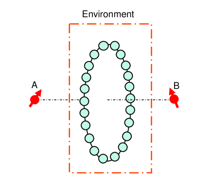
Figure 1: (Color online) The schematic diagram of two external interacting spin qubits symmetrically coupled to the environment described as an XY spin chain with Dzyaloshinsky-Moriya term.

II Model and solution

The quantum system we consider consists of two interacting qubits $s_{A}^{z}$ and $s_{B}^{z}$ coupled to a spin environment $E$. The environment is composed by $N$ spin-1/2 particles with periodic boundary condition, which can be described by one-dimensional XY spin chain with DM interaction Lieb-AnnPhys-1961 . The schematic diagram of the quantum open system is shown in Fig. 1. The corresponding Hamiltonian is given by

$$H=H_{E}^{\lambda}+H_{AB}+H_{I},$$ (1)

with

$$H_{E}^{\lambda} = \sum_{j=1}^{N}\left(\frac{1+\gamma}{2}\sigma_{j}^{x}\sigma_{j+1}^{x}+\frac{1-\gamma}{2}\sigma_{j}^{y}\sigma_{j+1}^{y}+\lambda\sigma_{j}^{z}\right)$$ (2)

$$+\sum_{j=1}^{N}\vec{D}\cdot(\vec{\sigma}_{j}\times\vec{\sigma}_{j+1}),$$

$$H_{AB} = Js_{A}^{z}s_{B}^{z},$$ (3)

$$H_{I} = g(s_{A}^{z}+s_{B}^{z})\sum_{j=1}^{N}\sigma_{j}^{z},$$ (4)

where $\sigma_{j}^{a}$ ($a=x$, $y$, $z$) is the Pauli matrix at site $j$. The parameters $\gamma$ and $\lambda$ characterize the anisotropy of the self-Hamiltonian and the intensity of the magnetic field applied along the $z$ axis, respectively. Here, such self-Hamiltonian $H_{E}^{\lambda}$ comprises DM term, which is an antisymmetric spin coupling. The DM interaction often arises from a mixture of superexchange and spin-orbit coupling in low-dimensional magnetic materials Dzyaloshinsky ; Moriya . For analytical solvability, we assume that the $\vec{D}$ vector is imposed along the $z$ direction., i.e., $\vec{D}=D\vec{z}$. The strength of interaction between the system qubits is given by $J(>0)$, and the coupling between the system qubits and the surrounding spin chain is denoted by $g$.

Since $[H_{AB},H_{I}]=0$, Hamiltonian (1) can be rewritten as

$$H=\sum_{\mu=1}^{4}\varepsilon_{\mu}|\phi_{\mu}\rangle\langle\phi_{\mu}|\otimes H_{E}^{\lambda_{\mu}},$$ (5)

where $|\phi_{\mu}\rangle$ $(\mu=1,\ldots,4)$ is the $\mu$th eigenstate of $H_{AB}$ with eigenvalue $\varepsilon_{\mu}$. Under these bases, the coupling $H_{I}$ between the qubits and spin chain exerts an extra magnetic field $\xi_{\mu}$ on the spin bath $H_{E}^{\lambda}$, and then gives rise to an effective qubit-dressed Hamiltonian $H_{E}^{\lambda_{\mu}}$ with magnetic field $\lambda_{\mu}=\lambda+\xi_{\mu}$. It is easy to find that

$$\xi_{1}=g,\quad\xi_{2}=\xi_{3}=0,\quad\xi_{4}=-g.$$ (6)

The Hamiltonian $H_{E}^{\lambda_{\mu}}$ can be diagonalized by following the standard procedures. The Jordan-Wigner transformation Jordan-Zphys-1928 ; Sachdev

$$\sigma_{j}^{+} =\exp\left[i\pi\sum_{i=1}^{j-1}f_{i}^{\dagger}f_{i}\right]f_{j}=\prod_{i=1}^{j-1}\sigma_{i}^{z}f_{j},$$

$$\sigma_{j}^{-} =\exp\left[-i\pi\sum_{i=1}^{j-1}f_{i}^{\dagger}f_{i}\right]f_{j}^{\dagger}=\prod_{i=1}^{j-1}\sigma_{i}^{z}f_{j}^{\dagger},$$

$$\sigma_{j}^{z} =1-2f_{j}^{\dagger}f_{j},$$ (7)

maps spin chain to one-dimensional spinless fermionic model with creation and annihilation operators as follows

$$H_{E}^{\lambda_{\mu}} =\sum_{j=1}^{N-1}\Bigg{[}(1-2iD)f_{j}^{\dagger}f_{j+1}+(1+2iD)f_{j+1}^{\dagger}f_{j}$$

$$+\gamma\left(f_{j}^{\dagger}f_{j+1}^{\dagger}+f_{j+1}f_{j}\right)+\lambda_{\mu}\left(1-2f_{j}^{\dagger}f_{j}\right)\Bigg{]}$$

$$+\Bigg{[}(1-2iD)f_{N}^{\dagger}f_{1}+(1+2iD)f_{1}^{\dagger}f_{N}$$

$$+\gamma\left(f_{N}^{\dagger}f_{1}^{\dagger}+f_{1}f_{N}\right)\Bigg{]}\exp(i\phi)+\lambda_{\mu}\left(1-2f_{N}^{\dagger}f_{N}\right).$$ (8)

An extra phase $\phi$ = $\pi(\sum_{j=1}^{N}f_{j}^{\dagger}f_{j}+1)$ appears on the chain boundary due to phase accumulation of the Jordan-Wigner transformation.

Next discrete Fourier transformation is introduced to convert the fermionic operators from real space to momentum space by defining

$$d_{k}=\frac{1}{\sqrt{N}}\sum_{j}e^{ikj}f_{j},\text{ \ \ }d_{k}^{\dagger}=\frac{1}{\sqrt{N}}\sum_{j}e^{-ikj}f_{j}^{\dagger},$$ (9)

with the discrete momentums as

$$k=\frac{(2n\pi+\phi)}{N},\quad n=-\frac{N}{2},-\frac{N}{2}+1,...,\frac{N}{2}-1.$$ (10)

After that, the Hamiltonian becomes

$$H_{E}^{\lambda_{\mu}} = \sum_{k}\left(2\cos k-2\lambda_{\mu}-4D\sin k\right)d_{k}^{\dagger}d_{k}$$ (11)

$$+i\gamma\sin k\left(d_{-k}^{\dagger}d_{k}^{\dagger}+d_{-k}d_{k}\right)+N\lambda_{\mu}.$$

The diagonalized form is achieved by Bogoliubov transformation which defines quasiparticle creation (annihilation) operator $b_{k,\lambda_{\mu}}^{\dagger}$ ($b_{k,\lambda_{\mu}}$) as

$$d_{k} =\cos\frac{\theta_{k}^{\lambda_{\mu}}}{2}b_{k,\lambda_{\mu}}+i\sin\frac{\theta_{k}^{\lambda_{\mu}}}{2}b_{-k,\lambda_{\mu}}^{\dagger},$$

$$d_{k}^{\dagger} =\cos\frac{\theta_{k}^{\lambda_{\mu}}}{2}b_{k,\lambda_{\mu}}^{\dagger}-i\sin\frac{\theta_{k}^{\lambda_{\mu}}}{2}b_{-k,\lambda_{\mu}},$$ (12)

with the angle $\theta_{k}^{\lambda_{\mu}}$ defined by

$$\tan\theta_{k}^{\lambda_{\mu}}=\frac{-\gamma\sin k}{\lambda_{\mu}-\cos k}.$$ (13)

Consequently, the dressed self-Hamiltonian is unitarily equivalent to such diagonal form

$$H_{E}^{\lambda_{\mu}}=\sum_{k}\Omega_{k}^{\lambda_{\mu}}(b_{k,\lambda_{\mu}}^{\dagger}b_{k,\lambda_{\mu}}-\frac{1}{2}),$$ (14)

where

$$\Omega_{k}^{\lambda_{\mu}}(k)=2\sqrt{\left(\lambda_{\mu}-\cos k\right)^{2}+\left(\gamma\sin k\right)^{2}}-4D\sin k.$$ (15)

The ground state $|G\rangle_{\lambda_{\mu}}$ has no quasiparticle for arbitrary $k$, i.e., $b_{k,\lambda_{\mu}}|G\rangle_{\lambda_{\mu}}=0$. Due to the relation $b_{k,\lambda_{\mu}}=\cos(\theta_{k}^{\lambda_{\mu}}/2)$ $d_{k}-$$i\sin(\theta_{k}^{\lambda_{\mu}}/2)d_{-k}^{\dagger}$, $|G\rangle_{\lambda_{\mu}}$ can be written as

$$|G\rangle_{\lambda_{\mu}}=\prod_{k>0}\left(\cos\frac{\theta_{k}^{\lambda_{\mu}}}{2}|0\rangle_{k}|0\rangle_{-k}+i\sin\frac{\theta_{k}^{\lambda_{\mu}}}{2}|1\rangle_{k}|1\rangle_{-k}\right),$$ (16)

where $|0\rangle_{k}$ and $|1\rangle_{k}$ are the vacuum and single excitation of the $k$th mode $d_{k}$, respectively. With these analytical expressions, we can straightforwardly derive the time evolution of arbitrary initial state and obtain the reduced density matrix of the two-qubit system, and then examine the effect of the environment. Suppose that at time $t=0$ the qubits are completely disentangled from the environment, i.e., the global system wave function is given by

$$|\Psi(0)\rangle=|\phi(0)\rangle_{AB}\otimes|\phi(0)\rangle_{E}.$$ (17)

Clearly, governed by the Hamiltonian (1), the state at time $t$ is given by $|\Psi(t)\rangle=U(t)|\Psi(0)\rangle$, where $U(t)=\exp(-iHt)$ is the evolution operator of the composite system. The reduced density matrix of the two-qubit system is obtained

$$\rho_{A,B} =\text{{Tr}}_{E}(|\Psi(t)\rangle\langle\Psi(t)|)$$

$$=\text{{Tr}}_{E}(e^{-iHt}|\Psi(0)\rangle\langle\Psi(0)|e^{iHt})$$

$$=\sum_{\mu,\nu=1}^{4}c_{\mu}(t)c_{\nu}^{\ast}(t)F_{\mu\nu}(t)|\phi_{\mu}\rangle\langle\phi_{\nu}|,$$ (18)

where

$$c_{\mu}=e^{-i\varepsilon_{\mu}t}\langle\phi_{\mu}|\Phi(0)\rangle_{AB},$$ (19)

and the decoherence factors are

$$F_{\mu\nu}(t)={}_{E}\langle\phi(0)|\exp(iH_{E}^{\lambda_{\nu}}t)\exp(-iH_{E}^{\lambda_{\mu}}t)|\phi(0)\rangle_{E}.$$ (20)

We assume that the two qubits in $AB$ system initially stem from a separable state, i.e., $|\phi(0)\rangle_{AB}=(|0\rangle+|1\rangle)/\sqrt{2}\otimes(|0\rangle+|1\rangle)/\sqrt{2}$, where $|0\rangle$ and $|1\rangle$ denote the spin up and down, respectively. The initial state of the environment is supposed as the ground state of $H_{E}^{\lambda}$, i.e., $|\phi(0)\rangle_{E}=|G\rangle_{\lambda}$. By tedious calculation cheng ; yuan07 , we have

$$F_{\mu\nu}(t) ={}_{\lambda}\langle G|e^{iH_{E}^{\lambda_{\nu}}t}e^{-iH_{E}^{\lambda_{\mu}}t}|G\rangle_{\lambda}$$

$$=\prod_{k>0}\cos\Theta_{k}^{\lambda_{\mu}}\cos\Theta_{k}^{\lambda_{\nu}}e^{i(\Omega_{k}^{\lambda_{\mu}}-\Omega_{k}^{\lambda_{\nu}})t}\cos(\Theta_{k}^{\lambda_{\mu}}-\Theta_{k}^{\lambda_{\nu}})$$

$$+\sin\Theta_{k}^{\lambda_{\mu}}\sin\Theta_{k}^{\lambda_{\nu}}e^{-i(\Omega_{k}^{\lambda_{\mu}}-\Omega_{k}^{\lambda_{\nu}})t}\cos(\Theta_{k}^{\lambda_{\mu}}-\Theta_{k}^{\lambda_{\nu}})$$

$$+\sin\Theta_{k}^{\lambda_{\mu}}\cos\Theta_{k}^{\lambda_{\nu}}e^{-i(\Omega_{k}^{\lambda_{\mu}}+\Omega_{k}^{\lambda_{\nu}})t}\sin(\Theta_{k}^{\lambda_{\mu}}-\Theta_{k}^{\lambda_{\nu}})$$

$$-\cos\Theta_{k}^{\lambda_{\mu}}\sin\Theta_{k}^{\lambda_{\nu}}e^{i(\Omega_{k}^{\lambda_{\mu}}+\Omega_{k}^{\lambda_{\nu}})t}\sin(\Theta_{k}^{\lambda_{\mu}}-\Theta_{k}^{\lambda_{\nu}}),$$ (21)

where $\Theta_{k}^{\lambda_{\mu}}=(\theta_{k}^{\lambda_{\mu}}-\theta_{k}^{\lambda})/2$ is the angle difference between the normal mode dressed by the system-environment interaction and the purely environment.

From Eq. (18), in the bases spanned by $\{|00\rangle,|01\rangle,|10\rangle,|11\rangle\}$, the reduced density matrix of the two-qubit system is obtained

$$\rho_{AB}(t)=\frac{1}{4}{\small\left(\begin{array}[]{cccc}1&e^{-\frac{iJt}{2}}F_{12}(t)&e^{-\frac{iJt}{2}}F_{13}(t)&F_{14}(t)\\ e^{\frac{iJt}{2}}F_{12}^{\ast}(t)&1&F_{23}(t)&e^{\frac{iJt}{2}}F_{24}(t)\\ e^{\frac{iJt}{2}}F_{13}^{\ast}(t)&F_{23}^{\ast}(t)&1&e^{\frac{iJt}{2}}F_{34}(t)\\ F_{14}^{\ast}(t)&e^{-\frac{iJt}{2}}F_{24}^{\ast}(t)&e^{-\frac{iJt}{2}}F_{34}^{\ast}(t)&1\end{array}\right).}$$ (22)

Some matrix elements can be further simplified for the choice of $\lambda_{\mu}$. For the case of Eq. (6), we have $\Theta_{k}^{\lambda_{2}}=\Theta_{k}^{\lambda_{3}}=0$, and also it is obvious that such relations hold: $F_{12}=F_{13}$, $F_{23}=1$, $F_{24}=F_{34}$. So there are three independent decoherence factors.

To investigate the entanglement dynamics of two qubits surrounding spin bath, rather than decoherence factor employed in Refs. cheng ; yuan07 , we utilize the concurrence directly Wootters , an entanglement measure for any bipartite system that relates to the two-site reduced density matrix $\rho$. The concurrence for two qubits is defined as

$$C(t)=\max\{0,\sqrt{\omega_{1}}-\sqrt{\omega_{2}}-\sqrt{\omega_{3}}-\sqrt{\omega_{4}}\},$$ (23)

where $\omega_{i}$ $(i=1,\ldots,4)$ are the eigenvalues in decreasing order of the auxiliary matrix $\zeta=\rho(\sigma_{y}\otimes\sigma_{y})\rho^{\ast}(\sigma_{y}\otimes\sigma_{y})$. Here $\rho^{\ast}$ denotes the complex conjugation of $\rho$ in the standard bases and $\sigma_{y}$ is the Pauli matrix. The concurrence varies from $C=0$ for a separable state (zero entanglement) to $C=1$ for a maximally entangled state.

III Entanglement dynamics of the two-qubit system

Before we consider the competition of system-bath coupling and two-qubit interaction, we first emphasize the following two limiting cases. On one hand, when there is no coupling between system and environment, i.e., $g=0$, we can get $\omega_{1}=\sin^{2}Jt/2$, $\omega_{2}=\omega_{3}=\omega_{4}=0$, and then $C(t)=|\sin Jt/2|$. It means the interaction between the qubits can generate an oscillating entanglement with period of $2\pi/J$. At $t=(2m+1)\pi/J$ ($m=0,1,2,...$), the state of the system reaches the maximum entanglement. On the other hand, when there is no interaction between the two qubits, the entanglement dynamics of the qubit system returns to the process of entanglement induced by the spin bath yi . The entanglement changes dramatically along the line of critical points of the spin bath. Now we investigate the influence of the spin bath during the process of entanglement generation. In Fig. 2, concurrence is plotted as a function of magnetic field $\lambda$ and time $t$ with $J=2,\gamma=1,D=0$ in weak-coupling ($g\ll 1$) region. It shows that the spin bath will weaken the entanglement generation when the coupling between system and environment is adiabatically turned on. Especially, the quantum phase transition of XY model at $\lambda=1$ will greatly enhance the decoherence, which coincides with the rapid decay of LE in an Ising model quan . It should be noted that we consider dynamics evolution of the system based on a finite-sized environment. To examine the effect of the chain length $N$ on the quantum entanglement evolution, we plot Fig. 3. It shows that the longer the spin chain, the more serious the attenuation at QCP. The concurrence displays oscillatory decay of time for $N=401$ and $801$. As the length of the chain increases, the maximum value of concurrence decreases, and the revival of the concurrence disappears. The inset of Fig. 3 shows that the maximum concurrence decays exponentially with the square root of chain length $N$. In addition, in weak-coupling region, for large $\lambda$, the concurrence restores the sine function versus time. It seems that the effect of system-bath coupling is insignificant. The reason is that the spin bath is polarized along $z$ axis in strong magnetic field. In this case, each spin is not entangled with the rest spins and the qubits sjgu1 ; sjgu2 . In other word, the ferromagnetic bath can be more or less thought of as classical. Therefore, it has negligible effect on qubits, and the interaction between qubits plays a dominant role in entanglement generation again, as shown in Fig. 2.

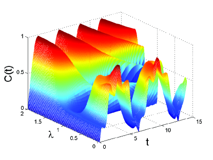
Figure 2: (Color online) Concurrence evolution versus $\lambda$ for $N=801$, $J=2$, $\gamma=1$, $D=0$ when there is weak-coupling between qubits and spin bath, i.e., $g=0.05$.

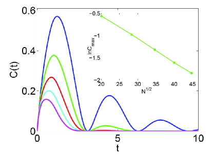
Figure 3: (Color online) Concurrence versus time $t$ is plotted for different chain length $N$ with $\lambda=1$, g=0.05, $\gamma$=1, J=2, D=0. From above to below, the lines correspond to $N$= 401, 801, 1201, 1601 and 2001. The logarithm of maximum concurrence versus $\sqrt{N}$ is shown in the inset.

Then we investigate the effect of DM interaction at QCP of the spin bath. In Fig. 4 (a)-(c), we display the concurrence against time $t$ under different $D$ with $\gamma$ equals to $0.8$, $0.6$ and $0.4$, respectively. We can see the maximum concurrence is enhanced by increasing $D$. The bigger the magnitude of $D$, the less time needed to reach the maximum concurrence. The growth of entanglement can be interpreted via the fact that the DM interaction arouses the strong planar quantum fluctuations. We would like to point out that the entanglement generation is suppressed at the QCP of spin bath as in Fig. 2, so the maximum concurrence can not reach unity. However, as the anisotropy parameter $\gamma$ decreases, the quantum fluctuations arising from the in-planar interactions become stronger kar , and then the two qubits in the presence of quantum fluctuations are more quantum correlated. In a word, the suppression of the entanglement at the QCP can be compensated both by increasing the DM interaction and by decreasing the anisotropy of the spin chain.

We now turn to the entanglement dynamics beyond the weak-coupling region. Fig. 5 shows the concurrence as a function of time and the coupling $g$. When the coupling $g$ increases, due to the decoherence of spin environment, the concurrence damps dramatically. Thus in the strong-coupling region, no entanglement is generated. However, it should be noted that in the vicinity of $g=\lambda=1$, the suppression of the entanglement generation at the quantum critical point is released. At some time entanglement emerges suddenly and reaches a maximum value in a short time. It can be easily concluded from Fig. 6 that the resonance peaks periodically appear at $t=m\pi/2$, where $m$ is an integer. We study the behavior of the resonance peaks with respect to parameters $D$ and $\gamma$. As shown in Fig. 6 (a), resonance peaks disappear quickly as $\gamma$ decreases, and there is no revival when $\gamma$ is less than certain threshold. A similar phenomenon builds up as the parameter $D$ increases, as shown in Fig. 6 (b). This reveals that these resonance peaks are highly sensitive to both the anisotropy parameter and the DM interaction strength.

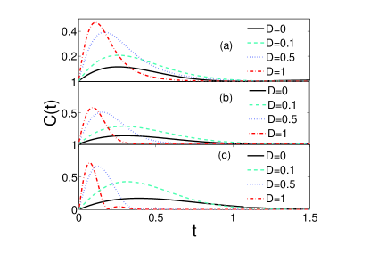
Figure 4: (Color online) Concurrence as a function of time $t$ under different $D$ with (a) $\gamma=0.8$, (b) $\gamma=0.6$, and (c) $\gamma=0.4$. We set other parameters as $\lambda=1.0$, $J=2$, $g=0.05$, and $N=2001$.

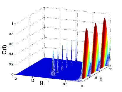
Figure 5: (Color online) Concurrence as a function of time $t$ and coupling parameter $g$ with $N=801$, where we set other parameters as $\lambda=1.0$, $J=2.0$, $\gamma=1$, and $D=0$.

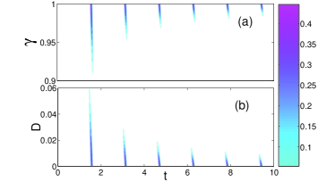
Figure 6: (Color online) Concurrence as a function of time $t$ and (a) the anisotropy parameter $\gamma$, (b) the intensity of the DM interaction $D$. We set other parameters as $N=801$, $g=\lambda=1.0$, $J=2.0$ with (a) $D=0$ and (b) $\gamma=1$.

In order to make a scrutiny into the resonance peaks, we rule out the effect of anisotropy and DM terms, i.e., $D=0$, $\gamma=1$. Now we have $\lambda_{1}=2\lambda$, $\lambda_{2}$ =$\lambda_{3}$ = $\lambda$, and $\lambda_{4}=0$. Under these parameters, Fig. 7 depicts the decoherence factors and concurrence against time in the resonance case $g=\lambda=1$. We can see that the decoherence factors $\left|F_{12}\right|$ and $\left|F_{14}\right|$ collapse to zero fleetly, while $\left|F_{24}\right|$ displays periodic revivals as time goes on. According to Eq. (23), the concurrence is dominated by $\left|F_{24}\right|$ when $\left|F_{12}\right|$ and $\left|F_{14}\right|$ decay to zero, and exhibits the similar behavior as $\left|F_{24}\right|$.

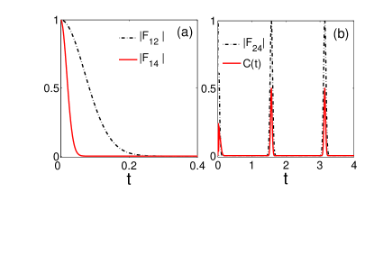
Figure 7: (Color online) Docoherence factor $|F_{\mu\nu}|$ and concurrence as a function of time $t$. We set other parameters as $N=801$, $g=\lambda=1.0$, $J=2.0$, $\ D=0$ and $\gamma=1$.

To illustrate why there are robust peaks of concurrence for $\gamma=1$ and $D=0$, let us give a heuristical explanation as follows. By Eq. (21), we have

$$F_{12}(t)=\prod_{k>0}e^{-i\Omega_{k}^{\lambda_{2}}t}\left[\cos^{2}(\Theta_{k}^{\lambda_{1}})e^{i\Omega_{k}^{\lambda_{1}}t}+\sin^{2}(\Theta_{k}^{\lambda_{1}})e^{-i\Omega_{k}^{\lambda_{1}}t}\right].$$

Such form of expression has been studied carefully in Refs. cheng ; Cucchietti1 ; Cucchietti2 . $|F_{12}(t)|$ shows a Gaussian decay with time for $\lambda=1$. Interestingly, the decoherence factor $F_{14}(t)=$
${}_{\lambda}\langle G|e^{iH_{E}^{\lambda_{4}}t}e^{-iH_{E}^{\lambda_{1}}t}|G\rangle_{\lambda}$ is similar to the decoherence factor in the spin-echo experiment in Ref. Cucchietti2 , and also the decay of $|F_{14}(t)|$ is Gaussian cheng , as shown in Fig. 7(a).

A remarkable difference arises from $F_{24}(t)$. From Eq. (21), we have

$$F_{24}(t) =\prod_{k>0}e^{i\Omega_{k}^{\lambda_{2}}t}\left[\cos^{2}(\Theta_{k}^{\lambda_{4}})e^{-i\Omega_{k}^{\lambda_{4}}t}+\sin^{2}(\Theta_{k}^{\lambda_{4}})e^{i\Omega_{k}^{\lambda_{4}}t}\right].$$

(25)

Due to the condition that $g=\lambda$, such Hamiltonian has an important feature: the spectra $\Omega_{k}^{\lambda_{4}}$ of all the modes are independent of momentum, i.e., $\Omega_{k}^{\lambda_{4}}=2$. Consequently, at $t=m\pi/2$ ($m=$0, 1, 2, $\ldots$), $F_{24}$$(m\pi/2)$=$\prod_{k>0}$$(-1)^{m}$$e^{im\Omega_{k}^{\lambda_{2}}\pi/2}$. The norm of $F_{24}(m\pi/2)$ is unity. Based on such analysis, at $t=m\pi/2$, we can approximatively set $F_{12}=0$, $F_{14}=0$, $F_{24}=1$ in Eq. (22), and thus we obtain $C(m\pi/2)=0.5$. For a tiny time deviation $\delta$ from resonance time $m\pi/2$, it arrives

$$|F_{24}(\delta)| =\prod_{k>0}\left|\cos^{2}(\Theta_{k}^{\lambda_{4}})e^{-2i\delta}+\sin^{2}(\Theta_{k}^{\lambda_{4}})e^{2i\delta}\right|$$

$$\simeq e^{-A\delta^{2}},$$ (26)

with $A=\sum_{k>0}(1-\cos(4\Theta_{k}^{\lambda_{4}}))$. In other words, the decoherence factor $F_{24}(t)$ will exponentially decay in a short time after deviating from the resonance time. Therefore, at $t\neq m\pi/2$, replacing $F_{12}$, $F_{14}$ and $F_{24}$ with zeros in Eq. (22), we get $C(t)=0$. It means that the entanglement generation is due to the presence of the momentum-independent spectrum structure. The flat band will also be destroyed when $\gamma$ is deviated from $1$ or $D$ is turned on, so the resonance peaks will be suppressed by varying $\gamma$ or $D$, as shown in Fig. 6. These interesting features are also confirmed in our numerical study. With regard to the parameters of $\gamma=1$, $D=0$ and $g=\lambda$, we obtain

$$A=\sum_{k>0}\frac{2\lambda^{2}\sin^{2}k}{\lambda^{2}-2\lambda\cos k+1}=\left\{\begin{array}[]{ll }\frac{N\lambda^{2}}{2},&\lambda<1,\\ \frac{N}{2},&\lambda\geq 1.\end{array}\right.$$ (29)

Thus, the width of spikes of $|F_{24}|$ in Fig. 7(b) is inversely proportional to $\sqrt{N}\lambda$ when $\lambda<1$, while it is inversely proportional to $\sqrt{N}$ when $\lambda\geq 1$. Since the concurrence has the same dependence as $F_{24}$, the resonance peaks at QCP will get sharper with the increase of chain length $N$. The peaks are robust even at the thermodynamic limit.

We want to emphasize that the behavior of $|F_{24}(t)|$ is universal for any $g=\lambda$, while the Gaussian decay for $F_{12(14)}(t)$ is only shown around QCP. When $g=\lambda\gg 1$, from the angle for Bogoliubov transformation in Eq. (13), we have

$$\theta_{k}^{\lambda} \approx 0,\quad\theta_{k}^{\lambda_{1}}\approx 0,\quad\theta_{k}^{\lambda_{2}}\approx 0,\quad\theta_{k}^{\lambda_{3}}\approx 0,$$ (30)

$$\theta_{k}^{\lambda_{4}} \approx \left\{\begin{array}[]{ll }\pi+k,&-\pi<k<0,\\ \pi-k,&0\leq k\leq\pi.\end{array}\right.$$ (33)

Consequently,

$$F_{12}(t) \approx \prod_{k>0}e^{i(\Omega_{k}^{\lambda_{1}}-\Omega_{k}^{\lambda_{2}})t},$$ (34)

$$F_{14}(t) \approx \prod_{k>0}e^{i\Omega_{k}^{\lambda_{1}}t}\left[\cos^{2}(\Theta_{k}^{\lambda_{4}})e^{-i\Omega_{k}^{\lambda_{4}}t}+\sin^{2}(\Theta_{k}^{\lambda_{4}})e^{i\Omega_{k}^{\lambda_{4}}t}\right].$$

Apparently, $|F_{12}(t)|\approx 1$, $F_{14}(t)/F_{24}(t)\approx F_{12}(t)$. It is notable that the form of Eq. (LABEL:Eq:F14) is similar with Eq. (25). Compared with $|F_{24}(t)|$ analyzed above, $|F_{12}(t)|$ should behave analogically, and spikes also spring up at $t=m\pi/2$. The situation is contrary to the case of $g=\lambda=1$. At $t\neq m\pi/2$, all the decoherence factors are zeros except $F_{12}(t)$, so the concurrence is dominated by $|F_{12}(t)|$, and thus the concurrence forms a flat platform structure, which remains at $C(t)=0.5$. As for $t=m\pi/2$, the concurrence shows exotic patterns, which are sensitive to the chain length $N$ and the amplitude of coupling $g$. Peaks and valleys emit from the platform at $t=m\pi/2$, where the system can reach maximum or zero concurrence state periodically, as depicted in Fig.8. According to the analysis above, we know that the width of peaks and valleys is inversely proportional to $\sqrt{N}$. It is observed that the width of peaks and valleys decreases as the chain length $N$ increase (see Fig. 8 (a)-(c)), and it is irrelevant to the coupling strength $g$ (see Fig. 8 (d)-(f)). For the region out of scope of QCP and strong coupling with $g=\lambda$, there exists competitive effect among these three decoherence factors.

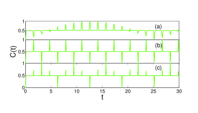
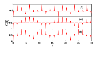
Figure 8: (Color online) Concurrence as a function of time $t$ for (a) N=201, (b) N=801, (c) N=1601 with $g$=$\lambda$=100, $J=2$, $\gamma=1$, and $D=0$; (d) $g$=$\lambda$=10, (e) g=$\lambda$=50, (f) g=$\lambda$=500 with $N=201$, $J=2$, $\gamma=1$, and $D=0$.

IV Conclusions

The investigation of decoherence of spin environment is an attractive topic in the entanglement dynamical process. In the paper, we have studied the entanglement dynamics in term of concurrence of two interacting spin qubits coupled to a general XY spin chain with DM interaction. When there is no coupling between two-qubit system and environment, the interaction between the qubits will generate entanglement as a sine function versus time. In the weak-coupling region, the entanglement generation is suppressed remarkably near the QCP of the spin bath. However, this suppression can be compensated both by increasing the DM interaction or by decreasing the anisotropy of the spin chain. Beyond the weak-coupling region, the system-bath coupling will make the entanglement in the system decay rapidly except for $g=\lambda$, where periodic resonance peaks of concurrence appear. By analyzing the decoherence factors, we attribute the appearance of resonance peaks to the emergence of the constant energy flat band. In such circumstances, increasing DM interaction or decreasing anisotropy will spoil the flatness of the band, and then the resonance peaks collapse. The effects of $\gamma$ and $D$ here seem contrary to case of weak coupling. The seemingly contradictory phenomena are originated from different mechanisms. The investigation of such model, in our opinion, may lead to several interesting phenomena in understanding decoherence in quantum open system. We hope that the simple analytical model described in this paper will assist us to gain further insight in QIP.

V ACKNOWLEDGMENTS

W. L. You is supported by start-up funding at Suzhou University under Grant No. Q4108907. Y. L. Dong acknowledges the support of the National Natural Science Foundation of China under Grant No. 10774108 and start-up funding at Suzhou University under Grant No. Q4108908.

References

- (1) C. H. Bennett and S. J. Wiesner, Phys. Rev. Lett. 69, 2881 (1992)
- (2) C. H. Bennett, G. Brassard, C. Crepeau, R. Jozsa, A. Peres, and W. K. Wootters, Phys. Rev. Lett. 70, 1895 (1993)
- (3) R. Jozsa and N. Linden, Proc. R. Soc. Lond. A 459, 2011 (2003)
- (4) L.-M. Duan, E. Demler, and M. D. Lukin, Phys. Rev. Lett. 91, 090402 (2003)
- (5) Michael J. Hartmann, Fernando G. S. L. Brandão, and Martin B. Plenio, Phys. Rev. Lett. 99, 160501 (2007)
- (6) T. J. Osborne, M. A. Nielsen, Phys. Rev. A 66, 032110 (2002)
- (7) A. Osterloh, L. Amico, G. Falci, and R. Fazio, Nature (London) 416, 608 (2002)
- (8) D. Gunlycke, V. M. Kendon, V. Vedral, and S. Bose, Phys. Rev. A 64, 042302 (2001)
- (9) M. C. Arnesen, S. Bose and V. Vedral, Phys. Rev. Lett. 87, 017901 (2001)
- (10) C. L. Zhang, S. Q. Zhu, and J. Ren, Phys. Lett. A 373 3522 (2009)
- (11) X. G. Wang, Phys. Rev. A 64, 012313 (2001)
- (12) K. M. O’Connor and W. K. Wootters, Phys. Rev. A 63, 052302 (2001)
- (13) S. J. Gu, S. S. Deng, Y. Q. Li, and H. Q. Lin, Phys. Rev. Lett. 93 086402 (2004)
- (14) H. T. Quan, Z. Song, X. F. Liu, P. Zanardi, and C. P. Sun, Phys. Rev. Lett. 96, 140604 (2006)
- (15) R. Orús, Phys. Rev. Lett. 100, 130502 (2008)
- (16) L. Amico, R. Fazio, A. Osterloh, and V. Vedral, Rev. Mod. Phys. 80, 517 (2008)
- (17) M. B. Plenio and S. F. Huelga, Phys. Rev. Lett. 88, 197901 (2002)
- (18) S. Bose, P. L. Knight, M. B. Plenio, and V. Vedral, Phys. Rev. Lett. 83, 5158 (1999)
- (19) X. X. Yi, H. T. Cui, and L. C. Wang, Phys. Rev. A 74, 054102 (2006)
- (20) Q. Ai, T. Shi, G. L. Long, and C. P. Sun, Phys. Rev. A 78, 022327 (2008)
- (21) W. H. Zurek, Phys. Today 44(10), 36 (1991)
- (22) T. Yu and J. H. Eberly, Science 323, 598 (2009)
- (23) A. Hutton and S. Bose, Phys. Rev. A 69, 042312 (2004)
- (24) F. M. Cucchietti, J. P. Paz, and W. H. Zurek, Phys. Rev. A 72, 052113 (2005)
- (25) W.-L You and W.-L. Lu, Phys. Lett. A 373, 1444 (2009)
- (26) Z. Sun, X. Wang, and C. P. Sun, Phys. Rev. A 75, 062312 (2007)
- (27) W. W. Cheng and J. M. Liu, Phys. Rev. A 79, 052320 (2009)
- (28) X. S. Ma, A. M. Wang, and Y. Cao, Phys. Rev. B 76, 155327 (2007)
- (29) X. S. Ma, H. S. Cong, J. Y. Zhang, and A. M. Wang, Eur. Phys. J. D, 48, 285 (2008)
- (30) E. Lieb, T. Schultz, and D. Mattis, Ann. Phys. 16, 407 (1961)
- (31) I. Dzyaloshinsky, J. Phys. Chem. Solids 4, 241 (1958)
- (32) T. Moriya, Phys. Rev. Lett. 4, 228 (1960)
- (33) P. Jordan and E. Wigner, Z. Phys. 47, 631 (1928)
- (34) S. Sachdev, Quantum Phase Transitions, (Cambridge University Press, Cambridge, UK, 2000)
- (35) Z. G. Yuan, P. Zhang, and S. S. Li, Phys. Rev. A 76, 042118 (2007)
- (36) W. K. Wootters, Phys. Rev. Lett. 80, 2245 (1998)
- (37) S. J. Gu, H. Q. Lin, and Y. Q. Li, Phys. Rev. A 68, 042330 (2003)
- (38) S. J. Gu, G. S. Tian, H. Q. Lin, Phys. Rev. A 71, 052322 (2005)
- (39) M. Kargarian, R. Jafari, and A. Langari, Phys. Rev. A 79, 042319 (2009)
- (40) F. M. Cucchietti, J. P. Paz, and W. H. Zurek, Phys. Rev. A 72, 052113 (2005)
- (41) F. M. Cucchietti, S. Fernandez-Vidal, and J. P. Paz, Phys. Rev. A 75, 032337 (2007)