A statistical method to determine open cluster metallicities

Abstract

Context. The study of open cluster metallicities helps to understand the local stellar formation and evolution throughout the Milky Way. Its metallicity gradient is an important tracer for the Galactic formation in a global sense. Because open clusters can be treated in a statistical way, the error of the cluster mean is minimized.

Aims. Our final goal is a semi-automatic statistical robust method to estimate the metallicity of a statistically significant number of open clusters based on Johnson $BV$ data of their members, an algorithm that can easily be extended to other photometric systems for a systematic investigation.

Methods. This method incorporates evolutionary grids for different metallicities and a calibration of the effective temperature and luminosity. With cluster parameters (age, reddening and distance) it is possible to estimate the metallicity from a statistical point of view. The iterative process includes an intrinsic consistency check of the starting input parameters and allows us to modify them. We extensively tested the method with published data for the Hyades.

Results. We selected sixteen open clusters within 1000 pc around the Sun with available and reliable Johnson $BV$ measurements. In addition, Berkeley 29, with a distance of about 15 kpc was chosen. For several targets we are able to compare our result with published ones which yielded a very good coincidence (including Berkeley 29).

Conclusions. A new method for the statistical determination of open cluster metallicities is presented and tested. It is quite robust against errors in effective temperature and luminosity calibration of the individual stars.

1 Introduction

Open clusters comprise of a local stellar population of with the same age and metallicity at a distinct distance from the Sun. Their study provides valuable information on the local as well as the global environment. In general, determining the age, distance and reddening for an open cluster by fitting isochrones is rather straightforward. However, the fourth free parameter, the metallicity, is either set to the solar value or is simply neglected.

Table 1: Distance, reddening and age starting values for the seventeen open clusters used in our analysis are presented in the left panel. In the right panel are the results obtained with our analysis.

Cluster		$d$	$E(B-V)$	log $t$	$d$	$E(B-V)$	log $t$	[Z]	[Fe/H]	[Fe/H]L
		[pc]	[mag]	[dex]	[pc]	[mag]	[dex]	[dex]	[dex]	[dex]
Alessi 13		110	0.040	8.720	110	0.040	8.720	0.027(7)	+0.17
Berkeley 29	C0650+169	14870	0.157	9.025	16440	0.200	9.380	0.007(2)	$-$0.48	$-$0.31(3)2
IC 4665	C1743+057	352	0.174	7.634	352	0.174	7.634	0.022(9)	+0.08	$-$0.03(4)2
Melotte 20	Alpha Per	185	0.090	7.854	185	0.090	8.050	0.028(7)	+0.18	$-$0.051
Melotte 25	Hyades	45	0.010	8.896	46	0.010	8.900	0.028(7)	+0.18	+0.13(5)2
Melotte 111	Coma Ber	96	0.013	8.652	81	0.013	8.800	0.018(8)	$-$0.03	$-$0.051
NGC 752	C0154+374	457	0.034	9.050	429	0.044	9.100	0.021(5)	+0.05	$-$0.081
NGC 1039	C0238+425	499	0.070	8.249	499	0.070	8.250	0.023(7)	+0.10	$-$0.301
NGC 2168	C0605+243	816	0.262	7.979	816	0.262	8.200	0.014(3)	$-$0.15	$-$0.161
NGC 2451 A	C0743$-$378	189	0.010	7.780	189	0.010	7.780	0.020(5)	+0.02
NGC 2451 B	C0743$-$378	302	0.055	7.648	302	0.055	7.570	0.019(4)	$-$0.01
NGC 2516	C0757$-$607	409	0.101	8.052	360	0.112	8.150	0.015(5)	$-$0.12	+0.061
NGC 2547	C0809$-$491	455	0.041	7.557	382	0.060	7.500	0.017(5)	$-$0.06	$-$0.161
NGC 2632	Praesepe	187	0.009	8.863	171	0.027	8.720	0.028(6)	+0.18	+0.141
NGC 6475	C1750$-$348	301	0.103	8.475	301	0.103	8.300	0.028(7)	+0.18	+0.14(6)2
NGC 7092	C2130+482	326	0.013	8.445	326	0.013	8.445	0.026(6)	+0.15
Stock 2	C0211+590	303	0.380	8.230	380	0.340	8.230	0.032(10)	+0.25
1: Chen et al (2003), 2: Magrini et al. (2009)

But the intrinsic metallicity of (proto-)stars is an important key parameter for our understanding of stellar formation and evolution. Metallicity already severely influences the cooling and collapse of ionized gas during the first stages of star formation (Jappsen et al. 2007). Machida (2008) showed that clouds with lower metallicity have a higher probability of fragmentation, indicating that the binary frequency is a decreasing function of cloud metallicity. On larger scales, clusters form and evolve significantly different in different environments, for example in the Milky Way and the Magellanic Clouds (Johnson et al. 1999).

Investigating the global properties of our Milky Way, a metallicity gradient throughout the Galactic disk was discovered several decades ago. The study of this gradient provides strong constraints on the mechanism of galaxy formation. Models show that star formation and the accretion history as functions of galactocentric distance strongly influence the appearance and the development of the abundance gradients (Chiappini et al. 2001). Relevant studies either use stellar data, for example those of Cepheids (Andrievsky et al. 2004, Cescutti et al. 2007), or open clusters (Chen et al. 2003, Magrini et al. 2009) as well as globular clusters (Yong et al. 2008). The first approach is limited to the accurate distance estimation of field stars and the uncertainties of spectroscopic abundance analysis for very distant and therefore faint objects, whereas metallicity compilations of open clusters (for example Chen et al. 2003) are normally based on rather inhomogeneous data sets.

We present a statistical method to estimate the metallicity of an open cluster based on photometric data sets; mostly on Johnson $BV$, for brighter stars also Geneva and Strömgren; and isochrone fitting to its members with an approximate knowledge about the clusters’ age, reddening and distance. The latter three parameters can be derived independently from different photometric data sets (Mermilliod & Paunzen 2003) or can be taken from catalogues (Paunzen & Netopil 2006).

The presented method can be easily extended to any other photometric system for which isochrones are available. This is especially interesting for all-sky-surveys like 2MASS (Cutrie et al. 2003) including homogeneous data of open clusters. Furthermore, it includes an intrinsic consistency check of the starting input parameters, hence it is superior to a standard isochrone fitting technique.

In Sect. 2 we present the basic method, its application to the Hyades and the target selection. In Sect. 3 we apply our method to sixteen additional open clusters. Several of them are compared to previous, independent investigations.

2 Aims, methods and target selection

Recently, Magrini et al. (2009) published metallicities for 45 open clusters on the basis of high resolution spectroscopy from the literature (mainly from red giants). However, it is still unclear whether the elemental abundances derived from highly evolved members of open clusters really represent those of stars still on the Main Sequence (MS hereafter). Another project in this respect is the Bologna Open Cluster Chemical Evolution project (Bragaglia 2008), dedicated primarily to old open clusters. Such surveys for open clusters are rather time consuming.

Our final goal is a semi-automatic statistically robust method to estimate the metallicity of a statistically significant sample of open clusters based on Johnson $BV$ data of its members. The method is designed in a way that it can easily be extended to other photometric systems like $VI_{\mathrm{c}}$. The influence of calibration errors of the basic astrophysical parameters for the individual stars should be minimized.

The procedure incorporates published evolutionary grids for different metallicities (Sect. 2.1) and a calibration for the effective temperature and luminosity (Sect. 2.2).

Targets were selected on the basis of well-known cluster parameters (distance, reddening and age) within 1000 pc. Furthermore, available Johnson $BV$ photometry to define a reliable MS for each cluster was another criterion. In order to test our method also at larger galactic distances, we additionally chose Berkeley 29 (about 15 kpc away from the Sun). For this old cluster, widely different cluster parameters are published. In total, we investigated seventeen open clusters in WEBDA that fulfil our requirements (Table 1). They are evenly distributed according to the reddening and age values.

The consecutive steps of our method, incorporating a test using the data of the Hyades are described in Sect. 2.3.

In the literature, metallicities are listed either as [Fe/H] or [Z] values. If not indicated otherwise, these parameters can be transformed using [Y] = 0.23 + 2.25[Z] derived by Girardi et al. (2000). For clarity, we list the corresponding values used for this paper in Table 2.

For the remainder of the paper the errors in the final digits of the corresponding quantity are given in parenthesis.

Table 2: Transformation of [Fe/H] to [Z].

[Fe/H]	[Z]	[Fe/H]	[Z]	[Fe/H]	[Z]
$-$0.729	0.004	$-$0.030	0.018	+0.253	0.032
$-$0.525	0.006	+0.019	0.020	+0.288	0.034
$-$0.387	0.008	+0.077	0.022	+0.312	0.036
$-$0.282	0.010	+0.116	0.024	+0.343	0.038
$-$0.224	0.012	+0.152	0.026	+0.371	0.040
$-$0.149	0.014	+0.185	0.028
$-$0.086	0.016	+0.225	0.030

2.1 The grid of evolutionary models

Our intention is to determine the metallicity on the basis of a theoretical Hertzsprung-Russell diagram, that means basically via $\log L/L_{\sun}$ versus $\log T_{\mathrm{eff}}$. Below we use the classical notation [H,He,Others] for [X,Y,Z] and/or [X:Y:Z]. The starting point is the evolutionary grid published by Claret & Gimenez (1998) available for [X:Z] = [0.63,0.73,0.80:0.01], [0.60,0.70,0.80:0.02] and [0.55,0.65,0.75:0.03]. The models allow us to take into account a known Helium abundance for open clusters (e.g. Hyades). Furthermore, they are very densely tabulated, justifying a linear interpolation. For [X:Y:Z] = [0.744:0.252:0.004] as well as [0.62:0.34:0.04], which are not available by Claret & Gimenez (1998), we used the models published by Schaller et al. (1992), Charbonnel et al. (1993) and Schaerer et al. (1993). The mentioned three grids are consistent within each other.

As a first step, the compatibility of the above mentioned grids was tested. For this purpose, the Zero-Age-Main-Sequence (ZAMS hereafter) of the model [X:Y:Z] = [0.68:0.30:0.02] was calculated and compared to the others. For the range 0 $\leq$ $\log L/L_{\sun}$ $\leq$ 3, with differences for $\log T_{\mathrm{eff}}$ between 0.006 and 0.010 dex which corresponds to $\leq$ 2% in $T_{\mathrm{eff}}$ only.

Table 3 shows the dependence of $\log T_{\mathrm{eff}}$ to [X:Y] for a constant [Z] value. In general, a mean [Y] value is assumed, which is related to the solar one. We were able to study published [Y] abundances for the case of the Hyades as described in Sect. 2.3. Perryman at al. (1998) derived [Y] = 0.26(2), whereas de Bruijne et al. (2001) list [Y:Z] = [0.285:0.024], taking into account new results for the Sun. The latter values agree with the Y-Z-relation published by Girardi et al. (2000). An uncertainty of a few percent for [Y] corresponds to only a small alteration of $\log T_{\mathrm{eff}}$ (Table 3), which is well in the range of the “grid differences”. An absolute error of 3% in the temperature determination ($\approx$ 200 K) is equal to $\Delta$[Y] = 0.1, which is well beyond the observed abundance uncertainties.

With [Y] = 0.23 + 2.25[Z] as published by Girardi et al. (2000), we chose the following models for our calibrations: [0.744:0.252:0.004], [0.73:0.26:0.01], [0.70:0,28:0.02], [0.65:0.32:0.03], and [0.62:0.34:0.04].

The final grid used for our analysis is listed in Table 5 in time steps of $\Delta$log $t$ = 0.2 for the complete metallicity and age range from 7.2 $\leq$ $\log t$ $\leq$9.6.

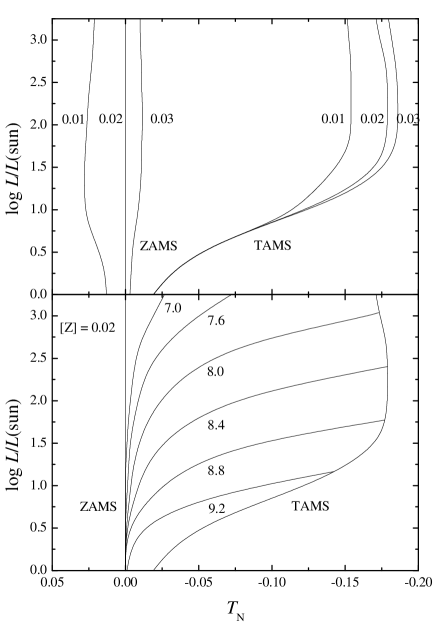
Figure 1: The evolutionary grid for different metallicities and ages versus the normalized effective temperature ($T_{\mathrm{N}}$).

Table 3: The ZAMS (left panel) and TAMS (right panel) for [Z] = 0.02 and different core Hydrogen abundances ($X_{\mathrm{c}}$).

$X_{\mathrm{c}}$	0.6	0.7	0.8	0.6	0.7	0.8
$\log L/L_{\sun}$	$\log T_{\mathrm{eff}}$			$\log T_{\mathrm{eff}}$
0.3	3.815	3.798	3.785	3.798	3.780	3.764
1.2	3.967	3.953	3.938	3.829	3.803	3.785
2.1	4.131	4.118	4.107	3.975	3.939	3.902
3.0	4.289	4.277	4.266	4.142	4.103	4.065

2.2 Calibration of the effective temperature and luminosity

For the calibration of the luminosity, an estimation for the bolometric correction $BC$ is vital. We took the results of Flower (1996), who lists $BC$ versus $\log T_{\mathrm{eff}}$ and ($B-V$) for MS stars and Giants. His Table 3 includes values for $-$0.35 $<$ ($B-V$) $<$ +1.8, which can be immediately compared to the calibration by Alonso et al. (1996) for [Fe/H] = 0. The differences $\Delta\log T_{\mathrm{eff}}$ between these two lists for +0.04 $<$ ($B-V$) $<$ +0.64 and the complete range of metallicities is less than 1%.

A polynomial interpolation of the data of Flower (1996) was performed, resulting in the following equations

$$BC = -0.238-5.561(\log T_{\mathrm{eff}}-4)$$

$$\qquad\qquad\qquad\qquad\mbox{for}\,\,4.00<\log T_{\mathrm{eff}}<4.25$$

$$BC = -0.243-5(\log T_{\mathrm{eff}}-4)-26(\log T_{\mathrm{eff}}-4)^{2}-$$

$$-33.33(\log T_{\mathrm{eff}}-4)^{3}$$

$$\qquad\qquad\qquad\qquad\mbox{for}\,\,3.76<\log T_{\mathrm{eff}}<4.00$$

$$BC = -0.155+2.84(B-V)-15.13(B-V)^{2}+$$

$$+25.57(B-V)^{3}$$

$$\qquad\qquad\qquad\qquad\mbox{for }-0.2<(B-V)<+0.1$$

$$BC = -0.030+0.491(B-V)-0.937(B-V)^{2}+$$

$$+0.055(B-V)^{3}$$

$$\qquad\qquad\qquad\qquad\mbox{for }+0.1<(B-V)<+0.8,$$

which are used to determine the $BC$. Finally the luminosity can be derived, taking $M_{\mathrm{\sun,Bol}}$ = 4.74 mag from Bessell et al. (1998) into account as

$$\log L/L_{\sun}=1.896-0.4(M_{\mathrm{V}}+BC)$$ (6)

within the listed range of parameters.

For establishing a metallicity calibration of an open cluster without narrow band and/or reddening independent photometry, we needed a well established and tested effective temperature calibration for ($B-V$). Alonso et al. (1996) published a $\log T_{\mathrm{eff}}$–[Fe/H]–($B-V$) calibration valid for +0.2 $<$ ($B-V$) $<$ +1.5 (F0 to K5) and $-$0.5 $<$ [Fe/H] $<$ +0.5 (suitable for open clusters) as follows

$$\Theta_{\mathrm{eff}}= + 0.541+0.533(B-V)+0.007(B-V)^{2}-$$ (7)

$$- 0.019(B-V)[\mathrm{Fe/H}]-0.047[\mathrm{Fe/H}]-$$

$$- 0.011[\mathrm{Fe/H}]^{2},$$

where $\Theta_{\mathrm{eff}}$ = 5040/$T_{\mathrm{eff}}$. We checked the results of the calibration with the values for Hyades members listed in Perryman at al. (1998) and found the following statistically significant correction term (see Sect. 2.3)

$$\log T_{\mathrm{eff}}^{\mathrm{corr}}-\log T_{\mathrm{eff}}=-0.009+0.012(B-V),$$ (8)

In the paper by Alonso et al. (1996), several comparisons with other calibrations can also be found.

For further interpolation we used normalized logarithmic effective temperature $T_{\mathrm{N}}$ values defined as

$$T_{\mathrm{N}}=\log T_{\mathrm{eff}}(\log L/L_{\sun})-\log T_{\mathrm{eff}}(\log L/L_{\sun})_{\mathrm{ZAMS(Z=0.02)}},$$ (9)

which simplified the calculations significantly. The basis of the normalization were the values of the ZAMS model for [0.70:0.28:0.02] as listed in Table 4. In other words, the evolution from the ZAMS for stars results always in a lower $T_{\mathrm{N}}$. If one intends to use other isochrone models, only the normalization ZAMS has to be altered. Figure 1 shows the grid for solar metallicity and different ages (lower panel). The upper panel shows the dependence of the ZAMS and Terminal-Age-Main-Sequence (TAMS hereafter) on the metallicity. The standard lines of $T_{\mathrm{N}}$ are much better separated for the metal poor than for the metal rich models. The differences for the region close to the TAMS are less pronounced. It is therefore essential to provide a profound knowledge about the cluster MS.

Table 4: The ZAMS of the evolutionary model used for the normalization.

$\log L/L_{\sun}$	$\log T_{\mathrm{eff}}$	$\log L/L_{\sun}$	$\log T_{\mathrm{eff}}$
$-$0.3	3.725	+1.8	4.064
+0.0	3.766	+2.1	4.118
+0.3	3.798	+2.4	4.171
+0.6	3.835	+2.7	4.225
+0.9	3.893	+3.0	4.277
+1.2	3.953	+3.3	4.327
+1.5	4.009

2.3 Test case: the Hyades

The Hyades were a natural choice for testing our method because they are well investigated and their metallicity is far from being settled. If our method is not robust at all, the result should be far off from the published values because the astrophysical parameters of the members are well known. In addition, we would like to point out that Melotte 20, Melotte 111, NGC 2632, and NGC 6475 are also included in this study. These open clusters are, in general, taken as “standards” in various papers. The main source of our investigation is the paper by Perryman at al. (1998), who extensively discussed the membership probabilities, distance, age and metallicity. They found a best isochrone fit with the model [0.716:0.26:0.024]. Here is an incomplete review of published [Fe/H] values

• Cameron (1985b): +0.08, photometry

• Berthet (1990): +0.081, photometry

• Boesgaard & Friel (1990): +0.127(22), high resolution spectroscopy

• Varenne & Monier (1999): $-$0.05(15), high resolution spectroscopy

• Dias et al. (2002): +0.17, mean value from publications

• Paulson et al. (2003): +0.13(1), high resolution spectroscopy

• Taylor & Joner (2005): +0.103(8), photometry and spectroscopy

showing the overall range of the estimates.

In Table 8 by Perryman at al. (1998), 40 Hyades members are listed, for which high resolution spectroscopy, photometry, parallaxes, effective temperatures, bolometric magnitudes and abundances are available. From this list, we excluded known spectroscopic binaries, chemically peculiar stars and giants which are too far from the ZAMS, which left us with 33 objects. These give a distance modulus of 3.33(1) or 46 pc for the cluster centre. The members are within 10 pc around the centre and necessitate the use of the individual distances for deriving the luminosities.

The reddening was set to 0.01 mag, which is an upper limit for the Hyades (de Bruijne et al. 2001). Any smaller value has no significant influence on the effective temperature calibration. The age of the Hyades is estimated as 625(50) Myr by Perryman at al. (1998), whereas An et al. (2007) give 550 Myr. In Dias et al. (2002) we find a significant higher value of 787 Myr.

The published metallicity can be estimated by the weights [0.60,0.36,0.04] of the following isochrones [0.70:0.28:0.02], [0.75:0.22:0.03] and [0.65:0.32:0.03], respectively. Figure 2 shows the isochrones for the Hyades with the apparent members. The lower panel shows the offset to the calibration of Alonso et al. (1996) according to Sect. 2.2 with (filled circles) and without (open circles) correction. According to this figure, we deduce log $t$ = 8.90 for our further analysis. The mean difference $\Delta\log T_{\mathrm{eff}}$ of the calibrated to the isochrone value for stars with $\log L/L_{\sun}$ $>$ 0 is $-$0.002(7).

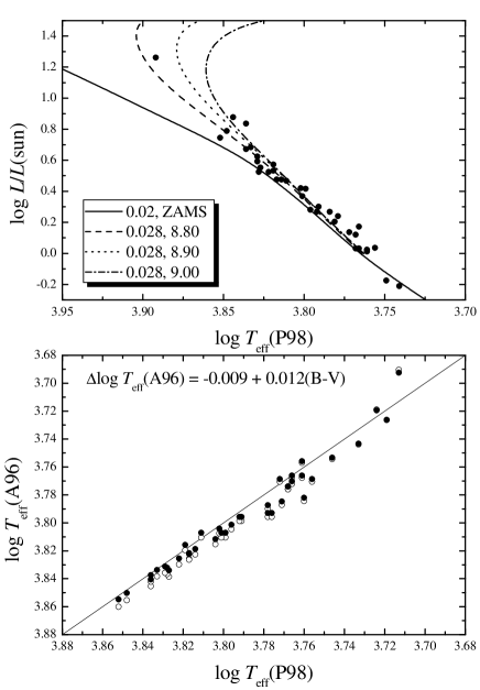
Figure 2: The isochrones for the Hyades with the members taken from Perryman at al. (1998, P98). The lower panel shows the offset to the calibration of Alonso et al. (1996, A96).

Below we list the consecutive steps of the iterative process of our method, the input parameters are $V$, $(B-V)$ and the grid $\log L/L_{\sun}$-$T_{\mathrm{N}}$-[Fe/H] (Table 5)

1. $\log T_{\mathrm{eff}}$ = f($(B-V)_{\mathrm{0}}$,[Fe/H]) [Eq. 7]

2. BC = f($(B-V)_{\mathrm{0}}$,$\log T_{\mathrm{eff}}$) [Eq. 2.2 - 2.2]

3. $\log L/L_{\sun}$ = f($M_{\mathrm{V}}$($V$,$d$,$E(B-V)$),BC) [Eq. 6]

4. $T_{\mathrm{N}}$ = f($\log T_{\mathrm{eff}}$,$\log L/L_{\sun}$) [Eq. 9, Table 4]

5. $[$Z$]$ from isochrones [Table 5]

The starting value for [Z] is always [Z]_☉. The transformation from [Z] into [Fe/H] can be done via the values listed in Table 2. If the input parameters $d$, $E(B-V)$, log $t$ and [Z] are correctly chosen, within the errors, the final $<$[Z]$>$ value has to be compatible with the individual starting value. If not, at least one iteration with different starting values has to be performed until no significant changes are seen. We wish to emphasize that this intrinsic consistency check makes our method superior to a standard isochrone fitting technique.

In total, the first iteration for 21 members of the Hyades gives mean metallicities between 0.029 and 0.032 for logarithmic ages between 8.8 and 9.0, respectively. These [Z] values are not compatible with the starting one. So we applied one iteration with [Fe/H] = 0.17, which is listed in Dias et al. (2002).

Taking the isochrone for log $t$ = 8.90 results in [Z] = 0.028(7), which is the best agreement between the starting and the mean value (see Fig. 2). The same procedure applying the corrected calibration by Alonso et al. (1996) gave [Z] = 0.025(9) as well as [Z] = 0.028(9), respectively. The corresponding median values ranged between 0.024 and 0.029 which excellently agrees with the derived means.

The age and metallicity is in concordance with the values listed by Dias et al. (2002). The test of our method with data for the Hyades gives a satisfying result. The grid of evolutionary models (Sect. 2.1) and the applied calibrations (Sect. 2.2) represent the test data very well.

Figure 3: The members of investigated clusters in the grid of isochrones. For clarity, only the grid for [Z] = 0.02 is included.

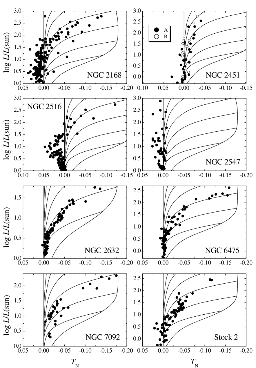
Figure 4: Same as Fig. 3.

Figure 5: The isochrone fits for investigated clusters.

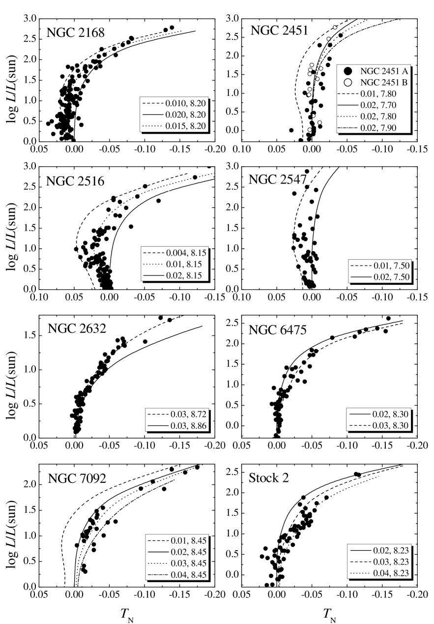
Figure 6: Same as Fig. 5.

2.4 Limitations

Before we discuss the apparent limitations of our method, we wish to stress again that the build-in intrinsic consistency check makes our method superior to a standard isochrone fitting technique.

On the other hand, there are no tests for the uniqueness of the final solution incorporated. One needs reliable input parameters for the age, reddening and distance. Looking at Table 1 we find “iterative changes” for the distance and reddening of up to 20%. Comparing these values with the results of Paunzen & Netopil (2006), we conclude that at least 60% of their evaluated data material fulfil these requirements. For the age, even a much larger spread can be treated by our method (see Berkeley 29 and NGC 2168).

The quality of published photometric data is highly divergent in the literature (Mermilliod & Paunzen 2003). In addition to the errors due to photon noise and the reduction process (for example point-spread-function fitting), the definition and transformation of the instrumental to a standard photometric systems, lacks all consistency much of the time. However, the high quality checks within WEBDA guarantees that the most divergent cases can be easily detected and rejected.

The MS of open clusters is shifted by a maximum of $M_{\mathrm{V}}$ = 0.754 mag caused by binaries of equal mass. Sharma et al. (2008) deduced a spread for it of about 0.2 mag in $(V-I)$. Hurley & Tout (1998) simulated the cluster MS with a realistic model of the binary fraction, concluding that there is a very pronounced “single star MS”, a much less pronounced one for a mass fraction equal to one and that in between there is only a sparse populated one. The misleading due to this effect can therefore in a statistically point-of-view be neglected.

One severe problem is the identification and choice of true cluster members. The most convenient way is to use kinematic data, like the proper motion and radial velocity for the individual stars. Recent data (Frinchaboy & Majewski 2008, Mermilliod et al. 2009) improved the membership criteria significantly in this respect. However, these data are mainly available for nearby open clusters. For more distant clusters, at least two statistical methods were developed to overcome the problem. Koposov et al. (2008) presented a technique to derive the clusters MS by counting the number of stars within segments of circles around the apparent cluster centre and plotting a density colour-magnitude diagram. With this method, they were able to detect new open clusters within the 2MASS survey. The other approach is to perform a statistically cleaning of the overall (cluster and field) colour-magnitude diagram with several assumptions about the stellar content for the line of sight (Piatti et al. 2009). Both methods proved to be very robust in a statistical sense. These algorithm could help to perform a pre-selection of bona-fide members for distant open clusters before applying our method to derive the metallicity and improved cluster parameters. Because our method has to be seen from a statistical point-of-view, the choice of “true” members may decrease the error, but does not influence the average value itself. Looking at Figs. 3 and 4, a clear and distinct MS can be seen for all open clusters. Even if there are apparent non-members at the MS, the result will be not statistically affected similar to a Hess-diagramm for isochrone fitting (Koposov et al. 2008).

3 Analysis of additional sixteen open cluster data

As a further step, we applied our method to sixteen additional open clusters (Table 1). The photometric data were taken from WEBDA. Figures 3 and 4 show the cluster data within the evolutionary grids for [Z] = 0.02 and the isochrone ages according to Fig. 1. The cluster parameters taken from WEBDA, mainly based on the catalogue by Dias et al. (2002), are listed in Table 1.

The separate isochrone fits are shown in Figs. 5 and 6, which we will now discuss in more detail. The summary of all results are listed in Table 1.

Alessi 13: The only investigation of this cluster was done by Kharchenko et al. (2005), who did not include any metallicity value on the basis of $BV$ from the ASCC2.5 catalogue. The Hertzsprung-Russell diagram shows a clear MS. Taking their cluster parameters results in [Z] = 0.027(7), similar to the Hyades.

Berkeley 29: With a distance of about 15 kpc, it is one of the most distant galactic open clusters known. The papers of Kaluzny (1994) and Tosi et al. (2004) suggest an higher age than listed in WEBDA. We got a value of [Z] = 0.007(2), which is in the range of that published by Magrini et al. (2009) deduced from red giant members. The derived age is between the values published by Dias et al. (2002; 1.06 Gyr) and Tosi et al. (2004; 3.4 to 3.7 Gyr) and fits the isochrones very well.

IC 4665: The photometric measurements especially for stars with $V$ $>$ 12.5 mag exhibit a significant scatter probably caused by the young age and differential reddening. This makes the determination of the MS rather difficult. We calculated a value of [Z] = 0.022(9).

Melotte 20: The published metallicity values range from $-$0.05 $<$ [Fe/H] $<$ +0.07 for this young and near cluster. For the first iteration, based on recent $UBV$ CCD photometry, we chose [Fe/H] = +0.20, which is supported by a $\delta$($U-B$)_0.6 of $-$0.03 for the members and the corresponding metallicity calibration from Cameron (1985b). The best isochrone fit was found for log $t$ = 8.05 and [Z] = 0.03. The mean values for about 60 stars for log $t$ = 7.8, 8.0 and 8.2 are [Z] = 0.031(7), 0.030(7) as well as 0.027(8), respectively. As described in Sect. 2.3, the higher metallicity makes an estimation for solar luminosity stars more uncertain. As for the Hyades, we excluded members with calculated [Z] $>$ 0.04 values resulting in [Z] = 0.028(7) or [Fe/H] = +0.18. Melotte 20 seems more metal rich and older than previously thought.

Melotte 111: This open cluster is well investigated with [Fe/H] = $-$0.05 according to Gratton (2000). The published distances range from 81 pc (Makarov 2003) to 96 pc (Dias et al. 2002). Because the metallicity is very well known, it is possible to estimate the best distance value. The colour-magnitude diagram shows a large scatter. Nevertheless, it is possible to establish an MS from which we derived $d$ = 96 pc and [Z] = 0.028(8) as well as $d$ = 81 pc and [Z] = 0.018(8), both with log $t$ = 8.80, respectively. The latter value of [Z] agrees very well with published ones from the literature. We therefore conclude that the lower distance value is the more probable one.

NGC 752: We used the parameters given by Anthony-Twarog et al. (2006) and Taylor (2007) for our analysis. Several publications indicate that NGC 752 exhibits a nearly solar metallicity. We find [Z] = 0.021(5) from data of 40 members.

NGC 1039: It is one of the clusters for which rather different metallicity values are published. There is a sufficient number of observed members to apply our method. Cameron (1985a) listed a metallicity of [Fe/H] = $-$0.291, whereas Schuler et al. (2003) deduced [Fe/H] = +0.07(4) from five “warm stars”. We investigated the isochrones for [Z] = 0.01, 0.02 and 0.03, which show that the metallicity value from Cameron (1985a) does not fit the Hertzsprung-Russell diagram. Our final result of [Z] = 0.023(7) agrees very well with that by Schuler et al. (2003).

NGC 2168: With a distance of approximately 820 pc from the Sun, NGC 2168 is the most distant cluster apart from Berkeley 29 of our target sample. It is a perfect test case for more distant open clusters because we find diverging published values ranging from 816 pc (Kharchenko et al. 2005) to 918 pc (Kalirai et al. 2003). Barrado y Navascues et al. (2001) list [Fe/H] = $-$0.21, whereas we calculated [Z] = 0.014(3) for the best isochrone fit for log $t$ = 8.20.

NGC 2451 A and B: Maitzen & Catalano (1986) were the first who suggested that NGC 2451 actually comprises of two separate clusters, which happen to lie in a common line of sight. This conclusion was proved by Röser & Bastian (1994) on the basis of kinematic data. Hünsch et al. (2003) estimated an age of 50 and 80 Myr, a distance of 206 and 370 pc and a reddening of 0.01 and 0.05 mag for the individual components. The rather low metallicity value of [Fe/H] = $-$0.50 published by Lyngå  & Wramdemark (1984) does not take into account the “binary nature” of this cluster and is most certainly incorrect (Hünsch et al. 2003). We included the data of both components in one plot to show the similar metallicities and the rather young ages. Our metallicity estimation is [Z] = 0.020(5) and [Z] = 0.019(4) for NGC 2451 A and B, respectively.

NGC 2516: The large number of members and peculiar stars made NGC 2516 a target of several detailed investigations. We used the cluster parameters listed by Sung et al. (2002) who included all up-to-date published data and new optical as well as X-ray observations. We found a best fit for log $t$ = 8.15 and derived [Z] = 0.015(5), which is compatible with the value mentioned before.

NGC 2547: We compared the cluster parameters published by Dias et al. (2002), Naylor et al. (2002), Lyra et al. (2006) and Kharchenko et al. (2005) using the appropriate isochrones. The best fit was obtained with the values from Naylor et al. (2002), which were used to calculate [Z] = 0.017(5).

NGC 2632: For Praesepe we found several metallicity estimates in the literature ranging from +0.04 to +0.19 (Gratton 2000). For the reddening, we used $E(B-V)$ = 0.027 mag (Taylor 2006), which fits the photometric data much better than the value (0.009) listed by Dias et al. (2001). The latter resulted in effective temperatures which were systematically two to three percent too low. For an age of log $t$ = 8.72 (An et al. 2007), we get [Z] = 0.028(6) which means that the metal content of Praesepe is similar to that of the Hyades.

NGC 6475: Meynet et al. (1993) list this cluster in their standard compilation with an age of log $t$ = 8.35, which is younger than the age (8.475) given in Dias et al. (2002). We found a best fit for log $t$ = 8.30 yielding [Z] = 0.028(7).

NGC 7092: The published cluster parameters by Robichon et al. (1999), Dias et al. (2002) and Kharchenko et al. (2005) agree within the errors very well, resulting in [Z] = 0.026(6).

Stock 2: The cluster parameters by Dias et al. (2002, Table 1) do not coincide with those by Kharchenko et al. (2005), who list a larger distance of 380 pc and a smaller reddening of 0.34 mag, but a comparable age. We checked both sets of cluster parameters and found a much better agreement using the ones by Kharchenko et al. (2005), which we took to estimate [Z] = 0.032(10).

In Table 1 we summarize our results and compare them with the cluster parameters from WEBDA. In addition, we list the [Fe/H] values either from Magrini et al. (2009) based on high resolution spectroscopy or Chen et al. (2003), which is a mean of the at that time published values. The latter did not examine the data individually to see whether there were important differences among the clusters in the different catalogues. So the values can only serve as a guideline.

From the complete sample of seventeen open clusters, we deduced a mean error of $\sigma$[Z] = 0.006 for the derived metallicities. Averaging the errors listed in Magrini et al. (2009) results in $\sigma$[Z] = 0.004. Therefore our method provides in a statistical sense a comparable error level, to that of high resolution spectroscopy.

4 Conclusion and outlook

The situation of a homogeneous metallicity determination of open clusters is still very unsatisfying. Recent compilations in this respect suffer from the bias introduced by averaging values from many different sources and applied techniques (e.g. isochrone fitting and spectroscopic determinations) as well as large uncertainties for single object estimations which yield a significant error of the means.

The overall metallicity of open clusters and their members is an important astrophysical parameter for the understanding and modelling of the formation and evolution from a local (stars, binary systems, etc.) and global (the Milky Way as Galaxy) point of view. The key observational constraint of the Galactic metallicity gradient, for example, is still very inaccurate. Results of open clusters should be compared to abundances determinations of star groups like Cepheids, or globular clusters to get a consistent and global picture.

We presented a statistically robust method to determine the cluster metallicity in an iterative way. With a rough estimate of the age, reddening and distance of the cluster, the algorithm iterates within normalized evolutionary grids (Schaller et al. 1992, Charbonnel et al. 1993, Schaerer et al. 1993, and Claret & Gimenez 1998) to find the best numerical fit of all free four cluster parameters. As input data, Johnson $BV$ measurements of members defining the MS of the individual cluster are needed. These data are then calibrated using a corrected effective calibration by Alonso et al. (1996) and the bolometric correction by Flower (1996). One major advantage of the proposed method is the statistical treatment of many objects simultaneously, which minimizes individual outliers as well as erroneous measurements.

Our method was demonstrated and tested with data from the Hyades yielding an excellent agreement with the published values. Using the photometric data from WEBDA, we have selected sixteen additional open clusters, namely Alessi 13, Berkeley 29, IC 4665, Melotte 20, Melotte 111 , NGC 752 , NGC 1039, NGC 2168, NGC 2451 A, NGC 2451 B, NGC 2516, NGC 2547, NGC 2632, NGC 6475, NGC 7092 and Stock 2, within a distance of 1000 pc (exception: Berkeley 29 with 15 kpc) around the Sun and applied our method to determine the overall mean metallicity. In addition, the published cluster parameters were checked and, if necessary, improved.

The algorithm can be employed in a semi-automatic way for a much larger sample of open clusters and can be extended to any other photometric system. As a next step, we will apply the algorithm to the data included in WEBDA to determine cluster metallicities for a statistical significant number of aggregates.

Appendix A Evolutionary grids

Here we list the complete evolutionary grids from Claret & Gimenez (1998), Schaller et al. (1992), Charbonnel et al. (1993) and Schaerer et al. (1993) used for this paper. They are normalized using the ZAMS model for [0.70:0.28:0.02], listed in Table 4, to the logarithmic effective temperature $T_{\mathrm{N}}$.

Table 5: The complete evolutionary grids in time steps of $\Delta$log $t$ = 0.2 used for this study. Within the individual isochrones, a linear interpolation was performed.

ZAMS						log $t$ = 7.2
Z	0.004	0.01	0.02	0.03	0.04	Z	0.004	0.01	0.02	0.03	0.04
$\log L/L_{\sun}$	$T_{\mathrm{N}}$					$\log L/L_{\sun}$	$T_{\mathrm{N}}$
$-$0.3		+0.020	+0.000	$-$0.001
+0.0	+0.019	+0.013	+0.000	$-$0.003	$-$0.004	+0.0	+0.019	+0.013	+0.000	$-$0.003	$-$0.004
+0.3	+0.026	+0.014	+0.000	$-$0.004	$-$0.007	+0.3	+0.026	+0.014	+0.000	$-$0.004	$-$0.007
+0.6	+0.035	+0.020	+0.000	$-$0.005	$-$0.013	+0.6	+0.035	+0.019	+0.000	$-$0.005	$-$0.013
+0.9	+0.042	+0.027	+0.000	$-$0.008	$-$0.024	+0.9	+0.045	+0.026	+0.000	$-$0.009	$-$0.025
+1.2	+0.049	+0.028	+0.000	$-$0.010	$-$0.027	+1.2	+0.049	+0.027	+0.000	$-$0.012	$-$0.028
+1.5	+0.054	+0.028	+0.000	$-$0.011	$-$0.027	+1.5	+0.053	+0.027	$-$0.001	$-$0.013	$-$0.029
+1.8	+0.056	+0.027	+0.000	$-$0.011	$-$0.027	+1.8	+0.053	+0.026	$-$0.002	$-$0.014	$-$0.030
+2.1	+0.055	+0.026	+0.000	$-$0.012	$-$0.027	+2.1	+0.049	+0.022	$-$0.004	$-$0.015	$-$0.031
+2.4	+0.050	+0.025	+0.000	$-$0.011	$-$0.026	+2.4	+0.043	+0.017	$-$0.007	$-$0.017	$-$0.034
+2.7	+0.046	+0.023	+0.000	$-$0.011	$-$0.024	+2.7	+0.035	+0.011	$-$0.011	$-$0.022	$-$0.043
+3.0	+0.044	+0.022	+0.000	$-$0.010	$-$0.021	+3.0	+0.026	+0.003	$-$0.018	$-$0.029	$-$0.048
+3.3		+0.021	+0.000	$-$0.010		+3.3		$-$0.007	$-$0.028	$-$0.038
+3.6		+0.019	+0.000	$-$0.009		+3.6		$-$0.021	$-$0.042	$-$0.053
log $t$ = 7.4						log $t$ = 7.6
Z	0.004	0.01	0.02	0.03	0.04	Z	0.004	0.01	0.02	0.03	0.04
$\log L/L_{\sun}$	$T_{\mathrm{N}}$					$\log L/L_{\sun}$	$T_{\mathrm{N}}$
						$-$0.3		+0.020	+0.000
+0.0	+0.019	+0.013	+0.000	$-$0.003	$-$0.004	+0.0	+0.019	+0.013	+0.000	$-$0.003	$-$0.004
+0.3	+0.026	+0.014	+0.000	$-$0.004	$-$0.007	+0.3	+0.026	+0.014	+0.000	$-$0.004	$-$0.007
+0.6	+0.035	+0.019	+0.000	$-$0.005	$-$0.013	+0.6	+0.035	+0.019	+0.000	$-$0.005	$-$0.013
+0.9	+0.045	+0.026	+0.000	$-$0.010	$-$0.025	+0.9	+0.045	+0.026	+0.000	$-$0.010	$-$0.025
+1.2	+0.049	+0.027	$-$0.001	$-$0.012	$-$0.028	+1.2	+0.049	+0.026	$-$0.001	$-$0.013	$-$0.029
+1.5	+0.053	+0.026	$-$0.002	$-$0.013	$-$0.029	+1.5	+0.052	+0.024	$-$0.003	$-$0.015	$-$0.031
+1.8	+0.051	+0.024	$-$0.003	$-$0.015	$-$0.031	+1.8	+0.049	+0.021	$-$0.006	$-$0.018	$-$0.034
+2.1	+0.046	+0.019	$-$0.007	$-$0.018	$-$0.034	+2.1	+0.042	+0.014	$-$0.011	$-$0.023	$-$0.040
+2.4	+0.038	+0.013	$-$0.011	$-$0.022	$-$0.041	+2.4	+0.031	+0.006	$-$0.017	$-$0.029	$-$0.046
+2.7	+0.028	+0.004	$-$0.018	$-$0.029	$-$0.045	+2.7	+0.018	$-$0.007	$-$0.029	$-$0.041	$-$0.059
+3.0	+0.016	$-$0.008	$-$0.029	$-$0.040	$-$0.057	+3.0	$-$0.002	$-$0.024	$-$0.048	$-$0.061	$-$0.079
+3.3		$-$0.022	$-$0.045	$-$0.056		+3.3		$-$0.050	$-$0.077	$-$0.091
+3.6		$-$0.047	$-$0.072	$-$0.087		+3.6		$-$0.104	$-$0.139	$-$0.162
						TAMS
						$\log L/L_{\sun}$		+3.769	+3.702	+3.642
						$T_{\mathrm{N}}$		$-$0.153	$-$0.168	$-$0.171
						$\log T_{\mathrm{eff}}$		+4.252	+4.226	+4.213
log $t$ = 7.8						log $t$ = 8.0
Z	0.004	0.01	0.02	0.03	0.04	Z	0.004	0.01	0.02	0.03	0.04
$\log L/L_{\sun}$	$T_{\mathrm{N}}$					$\log L/L_{\sun}$	$T_{\mathrm{N}}$
$-$0.3		+0.020	+0.000	+0.001		$-$0.3		+0.020	+0.000	+0.001
+0.0	+0.023	+0.013	+0.000	$-$0.003	$-$0.004	+0.0	+0.023	+0.013	+0.000	$-$0.003	$-$0.005
+0.3	+0.028	+0.014	+0.000	$-$0.004	$-$0.007	+0.3	+0.028	+0.014	+0.000	$-$0.004	$-$0.007
+0.6	+0.034	+0.019	+0.000	$-$0.005	$-$0.013	+0.6	+0.035	+0.018	$-$0.001	$-$0.005	$-$0.013
+0.9	+0.047	+0.025	$-$0.001	$-$0.011	$-$0.026	+0.9	+0.047	+0.024	$-$0.002	$-$0.012	$-$0.026
+1.2	+0.053	+0.024	$-$0.002	$-$0.014	$-$0.030	+1.2	+0.052	+0.022	$-$0.004	$-$0.016	$-$0.032
+1.5	+0.052	+0.022	$-$0.005	$-$0.018	$-$0.033	+1.5	+0.048	+0.018	$-$0.009	$-$0.022	$-$0.038
+1.8	+0.045	+0.017	$-$0.009	$-$0.022	$-$0.039	+1.8	+0.039	+0.011	$-$0.015	$-$0.029	$-$0.047
+2.1	+0.035	+0.008	$-$0.017	$-$0.030	$-$0.048	+2.1	+0.025	$-$0.003	$-$0.029	$-$0.043	$-$0.066
+2.4	+0.021	$-$0.005	$-$0.029	$-$0.041	$-$0.060	+2.4	+0.004	$-$0.023	$-$0.048	$-$0.063	$-$0.095
+2.7	+0.000	$-$0.024	$-$0.048	$-$0.062	$-$0.091	+2.7	$-$0.026	$-$0.055	$-$0.085	$-$0.104	$-$0.129
+3.0	$-$0.036	$-$0.054	$-$0.082	$-$0.100	$-$0.128	+3.0	$-$0.092	$-$0.126	$-$0.165
+3.3		$-$0.113	$-$0.144	$-$0.173
TAMS						TAMS
$\log L/L_{\sun}$	+3.447	+3.421	+3.371	+3.317	+3.222	$\log L/L_{\sun}$	+3.086	+3.076	+3.039	+2.987	+2.937
$T_{\mathrm{N}}$	$-$0.117	$-$0.151	$-$0.170	$-$0.179	$-$0.180	$T_{\mathrm{N}}$	$-$0.113	$-$0.152	$-$0.173	$-$0.182	$-$0.176
$\log T_{\mathrm{eff}}$	+4.239	+4.196	+4.168	+4.132	+4.141	$\log T_{\mathrm{eff}}$	+4.181	+4.140	+4.110	+4.092	+4.090

Table 5: continued

log $t$ = 8.2						log $t$ = 8.4
Z	0.004	0.01	0.02	0.03	0.04	Z	0.004	0.01	0.02	0.03	0.04
$\log L/L_{\sun}$	$T_{\mathrm{N}}$					$\log L/L_{\sun}$	$T_{\mathrm{N}}$
$-$0.3		+0.020	+0.000	+0.001		$-$0.3		+0.020	+0.000	+0.001
+0.0	+0.019	+0.013	+0.000	$-$0.003	$-$0.005	+0.0	+0.019	+0.013	+0.000	$-$0.003	$-$0.005
+0.3	+0.027	+0.013	+0.000	$-$0.004	$-$0.006	+0.3	+0.027	+0.013	$-$0.001	$-$0.004	$-$0.007
+0.6	+0.036	+0.017	$-$0.001	$-$0.007	$-$0.013	+0.6	+0.037	+0.017	$-$0.002	$-$0.006	$-$0.013
+0.9	+0.046	+0.022	$-$0.003	$-$0.014	$-$0.026	+0.9	+0.047	+0.019	$-$0.006	$-$0.017	$-$0.029
+1.2	+0.047	+0.019	$-$0.007	$-$0.020	$-$0.034	+1.2	+0.047	+0.015	$-$0.013	$-$0.026	$-$0.042
+1.5	+0.041	+0.013	$-$0.014	$-$0.028	$-$0.045	+1.5	+0.040	+0.003	$-$0.025	$-$0.040	$-$0.054
+1.8	+0.031	+0.000	$-$0.027	$-$0.041	$-$0.059	+1.8	+0.028	$-$0.019	$-$0.047	$-$0.063	$-$0.081
+2.1	+0.010	$-$0.023	$-$0.049	$-$0.064	$-$0.090	+2.1	+0.009	$-$0.058	$-$0.090	$-$0.108	$-$0.130
+2.4	$-$0.043	$-$0.057	$-$0.087	$-$0.106	$-$0.143	+2.4	$-$0.088	$-$0.142	$-$0.179
+2.7	$-$0.101	$-$0.132	$-$0.172
TAMS						TAMS
$\log L/L_{\sun}$	+2.762	+2.771	+2.729	+2.663	+2.613	$\log L/L_{\sun}$	+2.464	+2.442	+2.402	+2.343	+2.334
$T_{\mathrm{N}}$	$-$0.113	$-$0.154	$-$0.178	$-$0.185	$-$0.180	$T_{\mathrm{N}}$	$-$0.113	$-$0.154	$-$0.179	$-$0.186	$-$0.182
$\log T_{\mathrm{eff}}$	+4.126	+4.083	+4.052	+4.033	+4.032	$\log T_{\mathrm{eff}}$	+4.074	+4.025	+ 3.993	+3.975	+3.980
log $t$ = 8.6						log $t$ = 8.8
Z	0.004	0.01	0.02	0.03	0.04	Z	0.004	0.01	0.02	0.03	0.04
$\log L/L_{\sun}$	$T_{\mathrm{N}}$					$\log L/L_{\sun}$	$T_{\mathrm{N}}$
$-$0.3		+0.020	$-$0.001	+0.001		$-$0.3		+0.021	$-$0.002	+0.001
+0.0	+0.019	+0.012	$-$0.001	$-$0.003	$-$0.006	+0.0	+0.020	+0.012	$-$0.001	$-$0.003	$-$0.006
+0.3	+0.027	+0.013	$-$0.001	$-$0.004	$-$0.007	+0.3	+0.028	+0.012	$-$0.001	$-$0.004	$-$0.007
+0.6	+0.035	+0.015	$-$0.003	$-$0.008	$-$0.015	+0.6	+0.035	+0.013	$-$0.005	$-$0.011	$-$0.016
+0.9	+0.043	+0.019	$-$0.010	$-$0.023	$-$0.035	+0.9	+0.038	+0.008	$-$0.019	$-$0.032	$-$0.042
+1.2	+0.033	+0.006	$-$0.022	$-$0.037	$-$0.055	+1.2	+0.020	$-$0.011	$-$0.039	$-$0.056	$-$0.077
+1.5	+0.012	$-$0.015	$-$0.043	$-$0.061	$-$0.090	+1.5	$-$0.017	$-$0.050	$-$0.083	$-$0.104	$-$0.137
+1.8	$-$0.032	$-$0.056	$-$0.088	$-$0.107	$-$0.137	+1.8	$-$0.040	$-$0.151
+2.1	$-$0.100	$-$0.150
TAMS						TAMS
$\log L/L_{\sun}$	+2.135	+2.118	+2.082	+2.040	+1.981	$\log L/L_{\sun}$	+1.845	+1.802	+1.772	+1.736	+1.671
$T_{\mathrm{N}}$	$-$0.111	$-$0.154	$-$0.179	$-$0.186	$-$0.183	$T_{\mathrm{N}}$	$-$0.106	$-$0.153	$-$0.178	$-$0.185	$-$0.177
$\log T_{\mathrm{eff}}$	+4.017	+3.967	+3.936	+3.921	+3.918	$\log T_{\mathrm{eff}}$	+3.956	+3.922	+3.881	+3.866	+3.867
log $t$ = 9.0						log $t$ = 9.2
Z	0.004	0.01	0.02	0.03	0.04	Z	0.004	0.01	0.02	0.03	0.04
$\log L/L_{\sun}$	$T_{\mathrm{N}}$					$\log L/L_{\sun}$	$T_{\mathrm{N}}$
$-$0.3		+0.019	$-$0.002	+0.001		$-$0.3		+0.019	$-$0.003	+0.001
+0.0	+0.022	+0.011	$-$0.001	$-$0.003	$-$0.007	+0.0	+0.019	+0.011	$-$0.002	$-$0.004	$-$0.008
+0.3	+0.025	+0.011	$-$0.002	$-$0.005	$-$0.008	+0.3	+0.022	+0.009	$-$0.005	$-$0.008	$-$0.011
+0.6	+0.028	+0.008	$-$0.009	$-$0.016	$-$0.023	+0.6	+0.020	+0.001	$-$0.017	$-$0.025	$-$0.034
+0.9	+0.021	$-$0.005	$-$0.033	$-$0.047	$-$0.061	+0.9	$-$0.012	$-$0.032	$-$0.061	$-$0.075	$-$0.095
+1.2	$-$0.011	$-$0.044	$-$0.076	$-$0.096	$-$0.133	+1.2	$-$0.079
+1.5	$-$0.090	$-$0.145
TAMS						TAMS
$\log L/L_{\sun}$	+1.533	+1.516	+1.478	+1.411	+1.351	$\log L/L_{\sun}$	+1.242	+1.197	+1.165	+1.120	+1.057
$T_{\mathrm{N}}$	$-$0.099	$-$0.149	$-$0.171	$-$0.173	$-$0.167	$T_{\mathrm{N}}$	$-$0.090	$-$0.128	$-$0.145	$-$0.143	$-$0.134
$\log L/L_{\sun}$	+3.919	+3.863	+3.834	+3.819	+3.817	$\log L/L_{\sun}$	+3.873	+3.824	+3.800	+3.793	+3.793
log $t$ = 9.4						log $t$ = 9.6
Z	0.004	0.01	0.02	0.03	0.04	Z	0.004	0.01	0.02	0.03	0.04
$\log L/L_{\sun}$	$T_{\mathrm{N}}$					$\log L/L_{\sun}$	$T_{\mathrm{N}}$
+0.0	+0.019	+0.011	$-$0.003	$-$0.006	$-$0.011	+0.0	+0.018	+0.010	$-$0.004	$-$0.008	$-$0.014
+0.15	+0.019	+0.011	$-$0.005	$-$0.008	$-$0.013	+0.15	+0.017	+0.008	$-$0.008	$-$0.014	$-$0.020
+0.3	+0.018	+0.007	$-$0.008	$-$0.012	$-$0.017	+0.3	+0.015	+0.002	$-$0.016	$-$0.028	$-$0.037
+0.45	+0.014	+0.001	$-$0.014	$-$0.022	$-$0.029	+0.45	+0.008	$-$0.010	$-$0.029	$-$0.046
+0.6	+0.008	$-$0.012	$-$0.030	$-$0.040	$-$0.056	+0.6	$-$0.018	$-$0.040	$-$0.060
+0.75	$-$0.004	$-$0.034	$-$0.056	$-$0.070	$-$0.090
+0.9	$-$0.028	$-$0.075	$-$0.098
TAMS						TAMS
$\log L/L_{\sun}$	+0.982	+0.940	+0.908	+0.855	+0.778	$\log L/L_{\sun}$	+0.695	+0.650	+0.603	+0.538	+0.446
$T_{\mathrm{N}}$	$-$0.075	$-$0.090	$-$0.103	$-$0.103	$-$0.097	$T_{\mathrm{N}}$	$-$0.055	$-$0.060	$-$0.064	$-$0.064	$-$0.060
$\log L/L_{\sun}$	+3.839	+3.808	+3.785	+3.781	+3.778	$\log L/L_{\sun}$	+3.818	+3.795	+3.774	+3.771	+3.763