Singlet-triplet relaxation in multivalley silicon single quantum dots

Abstract

We investigate the singlet-triplet relaxation due to the spin-orbit coupling together with the electron-phonon scattering in two-electron multivalley silicon single quantum dots, using the exact diagonalization method and the Fermi golden rule. The electron-electron Coulomb interaction, which is crucial in the electronic structure, is explicitly included. The multivalley effect induced by the interface scattering is also taken into account. We first study the configuration with a magnetic field in the Voigt configuration and identify the relaxation channel of the experimental data by Xiao et al. [Phys. Rev. Lett. 104, 096801 (2010)]. Good agreement with the experiment is obtained. Moreover, we predict a peak in the magnetic-field dependence of the singlet-triplet relaxation rate induced by the anticrossing of the singlet and triplet states. We then work on the system with a magnetic field in the Faraday configuration, where the different values of the valley splitting are discussed. In the case of large valley splitting, we find the transition rates can be effectively manipulated by varying the external magnetic field and the dot size. The intriguing features of the singlet-triplet relaxation in the vicinity of the anticrossing point are analyzed. In the case of small valley splitting, we find that the transition rates are much smaller than those in the case of large valley splitting, resulting from the different configurations of the triplet states.

I INTRODUCTION

Spin-based qubits in semiconductor quantum dots (QDs) are believed to be a promising candidate for scalable quantum computation.scalable Among different kinds of QDs, GaAs ones have been extensively investigated in the past decade.koppens ; petta ; koppens2 ; petta2 ; sasaki ; meunier ; cheng ; shen ; jiang ; golovach ; taylor ; taylor2 ; hanson ; hanson2 ; amasha ; climente As reported, the spin decoherence, which is essential to know for genuine applications in such systems, is limited by the hyperfine interactionpaget ; pikus ; erlingsson ; khaetskii ; witzel ; yao ; zhang ; deng ; coish1 ; cywinski ; cywinski2 and the spin-orbit coupling (SOC)dresselhaus ; rashba together with the scattering.cheng ; shen ; jiang ; climente Recently, much attention has been given to silicon due to its outstanding spin coherence properties.culcer ; li ; prada ; pan ; liu ; shaji ; culcer2 ; xiao Specifically, the hyperfine coupling strength in natural silicon is two orders of magnitude weaker than that in GaAscoish2 and can be further reduced by isotopic purification.taylor3 In addition, the Dresselhaus SOCdresselhaus is absent in bulk silicon because of the existence of the bulk inversion symmetry. Although the interfaces of a confined system can introduce an interface inversion asymmetry (IIA),vervoort ; vervoort2 ; nestoklon the SOC due to this effect is still very small. Moreover, the absence of the piezoelectric interaction makes the electron-phonon scattering much weaker compared to that in III-V semiconductor QDs.li All these features suggest a long spin decoherence time in silicon QDs, which is of great help in realizing the operation of logic gates and the storage of information. Furthermore, as an indirect gap semiconductor, silicon has sixfold degenerate minima of the conduction band. This degeneracy can be splitted by strain or confinement in quantum wells into two parts: a double-degenerate subspace of lower energy and a fourfold-degenerate subspace of higher energy. The presence of the interfaces can further lift the twofold degeneracy by a valley splitting energy, which is strongly dependent on the size of the confinement structure.boykin ; friesen Moreover, the correlation effects in silicon are much stronger than those in GaAs due to the enhanced electron-electron Coulomb interaction, thanks to the reduced kinetic energy due to the larger effective mass. Thus, the physics in silicon is expected to be richer.

Very recently, spin-qubits utilizing the singlet-triplet (ST) states in silicon QDs have been actively investigated.culcer ; li ; prada ; pan ; liu ; shaji ; culcer2 ; xiao Culcer et al.culcer analyzed the feasibility of initialization and manipulation of ST qubits in double QDs, concentrating on the multivalley effect. With a large valley splitting, the exchange coupling was explicitly investigated by Li et al..li However, to the best of our knowledge, study on the ST relaxation in silicon QDs is rather limited.prada ; pan ; shaji ; xiao Prada et al.prada calculated the ST relaxation using the perturbation method with the lowest few levels, which has been shown to be inadequate to study the ST relaxation time.shen Moreover, the Coulomb interaction was not explicitly calculated in their work. However, the strong Coulomb interaction together with the SOC are of critical importance to determine the energies and wave functions of the eigenstates in QDs. Therefore, the diagonalization approach with a large number basis functions is required to guarantee the convergence of the energy spectrum and the ST relaxation rates.shen ; climente In the present work, we calculate the ST relaxation in silicon single QDs by explicitly including the Coulomb interaction and the multivalley band structure as well as the SOC,rashba ; nestoklon which is the key of the ST relaxation mechanism discussed in this work. In the calculation, we employ the exact diagonalization method and calculate the ST relaxation rate from the Fermi golden rule.cheng ; shen We first calculate the ST relaxation rate in silicon QDs with a parallel magnetic field (i.e., the Voigt configuration). Our theory successfully explains the recent experiment, by Xiao et al.xiao and suggests that the measurement corresponds the relaxation of the lowest singlet, with the dominant channel being the one associated with the lowest triplet. We further predict a peak in the magnetic-field dependence of the ST relaxation rate, resulting from the large spin mixing at the anticrossing point between the singlet and triplet states. Then we investigate the perpendicular magnetic-field (the Faraday configuration) dependence of the ST relaxation rate with different values of the valley splitting. In the situation of large valley splitting, the lowest singlet and three triplet states are all constructed by the lowest valley state. We find that the transition rates can be effectively manipulated by the magnetic field and dot size. We also find intriguing features in the vicinity of the anticrossing points. Moreover, we compare the relative contributions of the intravalley transverse acoustic (TA) and longitudinal acoustic (LA) phonons to the transition rates. In the case of small valley splitting, the eigenstates of the lowest two valleys contribute. We find the ST relaxation in this case is much slower than that in the large valley splitting one.

This paper is organized as follows. We set up the model and give the formalism in Sec. II. Then in Sec. III, we utilize the exact diagonalization method to obtain the energy spectrum and calculate the ST relaxation rates. Both parallel and perpendicular magnetic-field dependences of the ST relaxation rates are studied. The behavior of the transition rates in the vicinity of the anticrossing points is also discussed in this section. We summarize in Sec. IV.

II MODEL AND FORMALISM

In our model, we choose the lateral confinement as $V_{c}(x,y)=\frac{1}{2}m_{t}\omega_{0}^{2}(x^{2}+y^{2})$, with $m_{t}$ and $\omega_{0}$ representing the in-plane effective mass and the confining potential frequency.fock ; darwin The effective diameter can then be expressed as $d_{0}=\sqrt{\hbar\pi/m_{t}\omega_{0}}$. In the growth direction $[001]$, $V_{z}(z)$ is applied within the infinite-depth well potential approximation. Then the single-electron Hamiltonian with magnetic field ${\bf B}=B_{\perp}\hat{\bf z}+B_{\|}\hat{\bf x}$ is described by

$$H_{\rm e}=\frac{{P_{x}}^{2}+{P_{y}}^{2}}{2m_{t}}+\frac{{P_{z}}^{2}}{2m_{z}}+V({\bf r})+H_{\rm so}({\bf P})+H_{\rm Z}+H_{\rm v},$$ (1)

with $m_{z}$ representing the effective mass along the $z$-direction. $V({\bf r})=V_{c}+V_{z}$ and ${\bf P}=-i\hbar{\mbox{\boldmath$\nabla$\unboldmath}}+(e/c){\bf A}$, with ${\bf A}=(-yB_{\perp},xB_{\perp},2yB_{\|})/2$. $H_{\rm so}$ describes the SOC Hamiltonian, including the Rashba termrashba due to the structure inversion asymmetry and the term due to the IIA.vervoort ; vervoort2 ; nestoklon Then, one obtains

$$H_{\rm so}=a_{0}(P_{x}\sigma_{y}-P_{y}\sigma_{x})+b_{0}(-P_{x}\sigma_{x}+P_{y}\sigma_{y}),$$ (2)

where $a_{0}$ and $b_{0}$ stand for the strengths of the Rashba and IIA terms, respectively. The Zeeman splitting is given by $H_{\rm Z}=\frac{1}{2}g\mu_{B}(B_{\perp}\sigma_{z}+B_{\|}\sigma_{x})$ with $g$ being the Landé factor. Since the four in-plane valleys are separated from the two out-of-plane ones by a large energy gain, only the two out-of-plane valleys are relevant in the calculation. $H_{\rm v}$ in Eq. (1) describes the couplingboykin ; friesen between the valleys lying at $\pm\langle k_{0}\rangle$ along the $z$-axis with $\langle k_{0}\rangle=0.85(2\pi/a_{\rm Si})$. Here, $a_{\rm Si}=5.43\,\mathring{\rm A}$ is the lattice constant of silicon. Throughout this paper, one uses the subscripts “$z$” and “$\bar{z}$” to denote the valley at $\langle k_{0}\rangle$ and the one at $-\langle k_{0}\rangle$, respectively.

By solving the Schrödinger equation of the Hamiltonian $H_{0}=\tfrac{1}{2m_{t}}({P_{x}}^{2}+{P_{y}}^{2})+\tfrac{1}{2m_{z}}{{P_{z}}^{2}}+V({\bf r})$, one obtains the eigenvaluesfock ; darwin

$$E_{nln_{z}}=\hbar\Omega(2n+|l|+1)+\hbar l\omega_{B}+\frac{{n_{z}}^{2}{\pi}^{2}{\hbar}^{2}}{8m_{z}a^{2}},$$ (3)

where $\Omega=\sqrt{{\omega_{0}}^{2}+{\omega_{B}}^{2}}$ and $\omega_{B}={eB_{\perp}}/{(2m_{t})}$. $a$ represents the half-well width. Here, $n=0,1,2,...$ is the radial quantum number and $l=0,\pm 1,\pm 2,...$ represents the azimuthal angular momentum quantum number. The index $n_{z}$ denotes the subbands resulting from the confinement along the growth direction. The corresponding eigenfunctions read

$$F_{nln_{z}}({\bf r}) = N_{n,l}(\alpha r)^{|l|}e^{-(\alpha r)^{2}/2}e^{il\theta}L_{n}^{|l|}{\big{(}}(\alpha r)^{2}{\big{)}}$$ (6)

$$\mbox{}\times\left\{\begin{array}[]{ll}\frac{1}{\sqrt{a}}\sin[\frac{n_{z}\pi}{2a}(z+a)],&\mbox{$|z|\leq a$}\\ 0,&\mbox{otherwise},\end{array}\right.$$

with $N_{n,l}=\{{\alpha}^{2}n!/[\pi(n+|l|)!]\}^{1/2}$ and $\alpha=\sqrt{m_{t}\Omega/\hbar}$. $L_{n}^{|l|}$ is the generalized Laguerre polynomial. The wave functions in different valleys can then be expressed as $\phi_{nln_{z}}^{z,\bar{z}}=F_{nln_{z}}({\bf r})e^{\pm ik_{0}z}u_{z,\bar{z}}({\bf r})$, with $u_{z,\bar{z}}({\bf r})$ representing the lattice-periodic Bloch functions.culcer Here, we neglect the orbital effect of the parallel magnetic field by considering the strong confinement along the growth direction.

One can demonstrate that the overlap between the wave functions in different valleys is negligibly small, therefore only $H_{\rm v}$ is considered to contribute to the intervalley coupling in the present work. However, there still remain some controversies over the valley coupling nowadays.friesen ; saraiva ; chutia In this work, we take $\langle\phi_{nln_{z}}^{z,\bar{z}}|H_{\rm v}|\phi_{n^{\prime}l^{\prime}n_{z}}^{\bar{z},z}\rangle=\Delta^{1}_{n_{z}}\delta_{nn^{\prime}}\delta_{ll^{\prime}}$ and $\langle\phi_{nln_{z}}^{z,\bar{z}}|H_{\rm v}|\phi_{n^{\prime}l^{\prime}n_{z}}^{z,\bar{z}}\rangle=\Delta^{0}_{n_{z}}\delta_{nn^{\prime}}\delta_{ll^{\prime}}$, according to Ref. friesen, . Here, only the coupling element between the states with identical $n_{z}$ is given, since only the first subband is included in our calculation while the others are neglected due to the much higher energy. Including this intervalley coupling, the eigenstates become $\phi_{nln_{z}}^{\pm}=\frac{1}{\sqrt{2}}(\phi_{nln_{z}}^{z}\pm\phi_{nln_{z}}^{\bar{z}})$ with eigenvalues $E_{nln_{z}}^{\pm}=E_{nln_{z}}+\Delta_{n_{z}}^{0}\pm|\Delta_{n_{z}}^{1}|$. In these equations,

$$\Delta_{n_{z}}^{0} = \frac{V_{\rm v}{n_{z}}^{2}{\pi}^{2}{\hbar}^{2}}{4m_{z}a^{3}},$$ (7)

$$\Delta_{n_{z}}^{1} = \frac{V_{\rm v}{n_{z}}^{2}{\pi}^{2}{\hbar}^{2}\cos(2k_{0}a)}{4m_{z}a^{3}},$$ (8)

with $V_{\rm v}$ standing for the ratio of the valley coupling strength to the depth of quantum well.friesen

For a two-electron QD, the total Hamiltonian is given by

$$H_{\rm tot}=(H_{\rm e}^{1}+H_{\rm e}^{2}+H_{\rm C})+H_{\rm p}+H_{\rm ep}^{1}+H_{\rm ep}^{2}.$$ (9)

Here, the two electrons are labeled by $``1"$ and $``2"$. The electron-electron Coulomb interaction is described by $H_{\rm C}=\frac{e^{2}}{4\pi\epsilon_{0}\kappa|{\bf r_{1}}-{\bf r_{2}}|}$ with $\kappa$ representing the relative static dielectric constant. $H_{\rm p}=\sum_{{\bf q}\lambda}\hbar\omega_{{\bf q}\lambda}a_{{\bf q}\lambda}^{+}a_{{\bf q}\lambda}$ represents the phonon Hamiltonian with $\lambda$ and ${\bf q}$ denoting the phonon mode and the momentum respectively. The electron-phonon interaction Hamiltonian is given by $H_{\rm ep}=\sum_{{\bf q}\lambda}M_{{\bf q}\lambda}(a_{{\bf q}\lambda}^{+}+a_{-{\bf q}\lambda})e^{i{\bf q}\cdot{\bf r}}$.

We construct two-electron basis functions in the forms of either singlet or triplet based on the the single-electron eigenstates. For example, we use two single-electron spatial wave functions $|n_{1}l_{1}n_{z1}n_{v1}\rangle$ and $|n_{2}l_{2}n_{z2}n_{v2}\rangle$ (denoted as $|N_{1}\rangle$ and $|N_{2}\rangle$ for short; $n_{v}=\pm$) to obtain the singlet functions

$$|S^{(\Xi)}\rangle=(|\uparrow\downarrow\rangle-|\downarrow\uparrow\rangle)\otimes\begin{cases}\frac{1}{\sqrt{2}}|N_{1}N_{2}\rangle,&N_{1}=N_{2}\\ \frac{1}{2}(|N_{1}N_{2}\rangle+|N_{2}N_{1}\rangle),&N_{1}\not=N_{2},\end{cases}$$ (10)

and the triplet functions for $N_{1}\neq N_{2}$

$$|T_{+}^{(\Xi)}\rangle=\frac{1}{\sqrt{2}}(|N_{1}N_{2}\rangle-|N_{2}N_{1}\rangle)\otimes|\uparrow\uparrow\rangle,$$ (11)

$$|T_{0}^{(\Xi)}\rangle=\frac{1}{2}(|N_{1}N_{2}\rangle-|N_{2}N_{1}\rangle)\otimes(|\uparrow\downarrow\rangle+|\downarrow\uparrow\rangle),$$ (12)

$$|T_{-}^{(\Xi)}\rangle=\frac{1}{\sqrt{2}}(|N_{1}N_{2}\rangle-|N_{2}N_{1}\rangle)\otimes|\downarrow\downarrow\rangle.$$ (13)

Here, the spatial wave functions of the first and second electrons in $|NN^{\prime}\rangle$ are denoted as $N$ and $N^{\prime}$ in sequence. The superscript $(\Xi)$ denotes the valley configuration of each state. We define $\Xi=\pm$ for the valley indexes of single electron states $n_{v1}=n_{v2}=\pm$, and $\Xi=m$ for $n_{v1}\neq n_{v2}$.

Then, one can calculate the matrix elements of the Coulomb interaction, which can be expressed by

$$\langle N_{1}N_{2}|H_{\rm C}|N_{1}^{\prime}N_{2}^{\prime}\rangle=\frac{e^{2}}{16{\pi}^{2}\epsilon_{0}\kappa}\delta_{l_{1}+l_{2},l_{1}^{\prime}+l_{2}^{\prime}}\sum_{\gamma_{1},\gamma_{2},\gamma_{1}^{\prime},\gamma_{2}^{\prime}=z,\bar{z}}\eta_{n_{v1}}^{\gamma_{1}}\eta_{n_{v2}}^{\gamma_{2}}\eta_{n_{v1}^{\prime}}^{\gamma_{1}^{\prime}}\eta_{n_{v2}^{\prime}}^{\gamma_{2}^{\prime}}G(\phi_{n_{1}l_{1}n_{z1}}^{\gamma_{1}},\phi_{n_{2}l_{2}n_{z2}}^{\gamma_{2}},\phi_{n_{1}^{\prime}l_{1}^{\prime}n_{z1}^{\prime}}^{\gamma_{1}^{\prime}},\phi_{n_{2}^{\prime}l_{2}^{\prime}n_{z2}^{\prime}}^{\gamma_{2}^{\prime}}),$$ (14)

where the superscripts $\gamma_{i}$ and $\gamma_{i}^{\prime}$ run over the two valleys, $z$ and $\bar{z}$, with $\eta_{\pm}^{z}=1$ and $\eta_{+}^{\bar{z}}=-\eta_{-}^{\bar{z}}=1$. $G$ is given in detail in Appendix. One also calculates the SOC and Zeeman splitting terms, hence obtains the two-electron Hamiltonian, i.e., the terms in the bracket in Eq. (9). Then, the two-electron eigenvalues and eigenfunctions can be obtained by exactly diagonalizing the two-electron Hamiltonian. We identify a two-electron eigenstate as singlet (triplet) if its amplitude of the singlet (triplet) components is larger than 50 %.

From the Fermi golden rule, one can calculate the transition rate from the state $|i\rangle$ to $|f\rangle$, due to the electron-phonon scattering,

$$\Gamma_{i\rightarrow f} = \frac{2\pi}{\hbar}\sum_{{\bf q}\lambda}|M_{{\bf q}\lambda}|^{2}|\langle f|\chi|i\rangle|^{2}[\bar{n}_{{\bf q}\lambda}\delta(\epsilon_{f}-\epsilon_{i}-\hbar\omega_{{\bf q}\lambda})$$ (15)

$$\mbox{}+(\bar{n}_{{\bf q}\lambda}+1)\delta(\epsilon_{f}-\epsilon_{i}+\hbar\omega_{{\bf q}\lambda})],$$

in which $\chi({\bf q},{\bf r_{1}},{\bf r_{2}})=e^{i{\bf q}\cdot{\bf r_{1}}}+e^{i{\bf q}\cdot{\bf r_{2}}}$ and $\bar{n}_{{\bf q}\lambda}$ stands for the Bose distribution of phonons. In our calculation, the temperature is fixed at 0 K. Thus $\bar{n}_{{\bf q}\lambda}=0$ and only the second term contributes.

III NUMERICAL RESULTS

Since the piezoelectric interaction is absent in siliconli and the energy difference between the initial and final states discussed here is much smaller than the energies of the intervalley acoustic phonon and the optical phonon,pop one only needs to calculate the intravalley electron-acoustic phonon scattering due to the deformation potential. In the present work, both the TA and LA phonons are included. The corresponding matrix elements are $M_{\beta,{\rm intra},{\bf Q}}^{2}={\hbar D_{\beta}^{2}Q^{2}}/{(2d\Omega_{\beta,{\rm intra},{\bf Q}})}$ with $\beta$=LA/TA standing for the LA/TA phonon mode. Here, we take the mass density of silicon $d=2.33$ g/cm³.sonder The deformation potentials for the LA and TA phonons are $D_{{\rm LA}}=6.39$ eV and $D_{{\rm TA}}=3.01$ eV, respectively.pop The phonon energy $\Omega_{\beta,{\rm intra},{\bf Q}}=v_{\beta}Q$ with sound velocities $v_{\rm LA}=9.01\times 10^{5}$ cm/s and $v_{\rm TA}=5.23\times 10^{5}$ cm/s.pop In our calculation, we take $m_{t}=0.19m_{0}$ and $m_{z}=0.98m_{0}$ with $m_{0}$ being the free electron mass.dexter The Landé factor $g=2$,graeff the ratio $V_{\rm v}=7.2\times 10^{-11}$ m.friesen In the calculation, we employ the exact diagonalization method with the lowest $1516$ singlet and $4452$ triplet basis functions to guarantee the convergence of the energies and the transition rates.

One finds that the eigenstates composed by the two-electron basis functions with single valley state “$-$” are almost independent of those constructed by the ones with single valley state “$+$” and two valley states “$-$” and “$+$”. On the one hand, there is nearly no coupling between them due to the negligibly small intervalley Coulomb interactionli and overlap between the wave functions in different valleys. One can also demonstrate that the elements of the SOCs between the states with different valley indices vanish when only the first subband is included, regardless of the coupling strengths $a_{0}$ and $b_{0}$. On the other hand, the transition between them is almost forbidden because $\langle f|\chi|i\rangle$ in Eq. (15) is strongly suppressed thanks to the large intervalley wave vector $\langle 2k_{0}\rangle$ from the difference of the phases between different valleys. Therefore, the eigenstates are divided into three independent sets based on the valley indexes. It is noted that the energy of the eigenstate with valley configuration “$-$” is smaller than the corresponding levels with valley configurations “$+$” and “$m$” due to the contribution of the valley splitting.

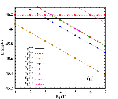
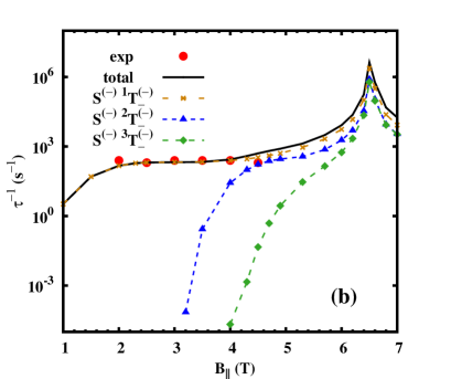
Figure 1: (Color online) (a) The lowest few energy levels vs. parallel magnetic field $B_{\|}$ in a single QD. Note that each of $|T_{0}^{(-)}\rangle$ and $|^{i}T_{-}^{(-)}\rangle$ ($i=1,2,3,6$) is double-degenerate. (b) Relaxation rates vs. the magnetic field. The red dots stand for the experimental data. ${\rm S^{(-)}\ }$ⁱ${\rm T_{-}^{(-)}}$ ($i=1$-$3$) denotes the sum of the relaxation rates from $|S^{(-)}\rangle$ to the two degenerate ⁱ${\rm T_{-}^{(-)}}$ levels. In the calculation, $2a=4.344$ nm and $d_{0}=56$ nm.

III.1 PARALLEL MAGNETIC-FIELD DEPENDENCE

Very recently, Xiao et al.xiao measured the ST relaxation time in Si/SiO₂ QDs under a magnetic field parallel to the interface of the heterostructure. They reported that the ST relaxation time only slightly fluctuates around 5 ms when the magnetic field increases from 2 to 4.5 T. In the experiment, the orbital level spacing is observed to be $\sim 0.4$ meV, corresponding to the effective diameter of the QD $d_{0}=56$ nm. However, some parameters such as the effective well width, the strengths of SOCs and the valley splitting are unavailable. Moreover, the channel of the relaxation process is not identified because of the uncertainty of the exact excited states spectrum in the experiment.xiao Here, we take advantage of our model to clarify the experiment situation. In the calculation, we assume the magnetic field along $x$-direction and take the relative static dielectric constant $\kappa=7.9$.li Since the valley splitting is strongly dependent on the effective well width according to Eq. (6), it is difficult to determine the energy spectrum without the knowledge of the exact well width. For a large valley splitting, the lowest levels are all constructed by the states with the single valley index “$-$”, and the energy difference between the adjacent levels is determined solely by the orbital level spacing and Zeeman splitting approximately. Therefore, the relaxation rate of each excited state can be calculated to identify the relaxation channel in the experiment. However, the lowest levels become more complicated for a small valley splitting because new levels with the valley index “$+$” become relevant. Fortunately, as said above, the inclusion of the states with valley configuration “$+$” or “$m$” has no observable influence on the relaxation of the states with the valley configuration “$-$”. In the following, we first study the large valley splitting case. We take 32 monoatomic layers of silicon along the growth direction, corresponding to the well width $2a=4.344$ nm ($2|\Delta_{n_{z}}^{1}|=0.83$ meV). The strengths of the Rashba SOC and IIA term are used as fitting parameters. We first calculate the energy spectrum since it is weakly dependent on the strengths of the SOCs. The lowest few levels, denoted as $|S^{(-)}\rangle$, $|T_{0}^{(-)}\rangle$ and $|^{i}T_{-}^{(-)}\rangle$ (spin down) ($i=1$-$6$) according to their major components, are plotted as function of the magnetic field in Fig. 1(a). As the magnetic field increases, the energies of $|S^{(-)}\rangle$ and $|T_{0}^{(-)}\rangle$ keep invariant while those of $|^{i}T_{-}^{(-)}\rangle$ ($i=1$-$6$) decrease due to the Zeeman splitting. The major component of $|S^{(-)}\rangle$ is constructed by the single-electron states $|01\rangle|0-1\rangle$ according to Eq. (10), and those of the triplet states $|^{4}T_{-}^{(-)}\rangle$ and $|^{5}T_{-}^{(-)}\rangle$ are given by $|01\rangle|0-1\rangle$ and $|00\rangle|10\rangle$ following Eq. (13), respectively. We find $|^{i}T_{-}^{(-)}\rangle$ ($i=1,2,3,6$) and $|T_{0}^{(-)}\rangle$ are all double-degenerate. The major components of the two levels of $|^{1}T_{-}^{(-)}\rangle$, $|^{2}T_{-}^{(-)}\rangle$, $|^{3}T_{-}^{(-)}\rangle$, and $|^{6}T_{-}^{(-)}\rangle$ are composed by the single-electron states $|00\rangle|0\pm 1\rangle$, $|0\pm 1\rangle|0\pm 2\rangle$, $|00\rangle|0\pm 2\rangle$ and $|10\rangle|1\pm 1\rangle$ in sequence. $|T_{0}^{(-)}\rangle$ is mainly constructed by the basis function involving $|00\rangle|0\pm 1\rangle$ also. Here, we only retain the quantum numbers $n$ and $l$ for short, because other quantum numbers of these single-electron states are all the same.

We then calculate the relaxation rates of these states due to phonon emission. Due to the low temperature in the experiment,xiao the relaxation rate at zero temperature can well represent the experimental data. We find that if one takes the Rashba SOC strength $a_{0}=-2.09$ m/s and the IIA term strength $b_{0}=-10.44$ m/s, the total relaxation rate of the state $|S^{(-)}\rangle$ fits the experimental data pretty well as shown in Fig. 1(b) (from 2 to 4.5 Tesla). The relaxation rates of other levels can not recover the experiment results. Specifically, the relaxation rate of $|T_{0}^{(-)}\rangle$ presents a peak at $B_{\|}\sim 3.45$ T (not shown in the figure) and those of $|^{i}T_{-}^{(-)}\rangle$ ($i=2$-$6$) relax too fast (in the magnitude of $\sim 1$ ns). Therefore, we conclude that the experimental data might correspond to the lifetime of the singlet $|S^{(-)}\rangle$. The rates of the major relaxation channels of $|S^{(-)}\rangle$ (involving ${\rm S^{(-)}}$ ⁱ${\rm T_{-}^{(-)}}$, $i=1$-$3$) are also plotted in Fig. 1(b). Interestingly, the calculation predicts a peak of the total relaxation rate at $B_{\|}\sim 6.5$ T, which should be checked by future experiments. Moreover, one also finds the significant increase of the total relaxation rate by increasing the magnetic field in the small magnetic field regime, i.e., below 2 T. Such rich magnetic-field dependences can be understood as follows. From the figure, we find that the dominant relaxation channel is the one from $|S^{(-)}\rangle$ to $|^{1}T_{-}^{(-)}\rangle$. In the small magnetic field regime, the energy of the phonon emmision of this channel (corresponding to the energy difference between $|S^{(-)}\rangle$ and $|^{1}T_{-}^{(-)}\rangle$) is small and linearly increases with the magnetic field, which lead to the significant enhancement of the transition.climente ; shen However, the transition rate becomes insensitive to the phonon energy since the value of $\langle f|\chi|i\rangle$ in Eq. (15) is suppressed for a large phonon momentum, then the transition rate only slightly varies beyond 2 T. This picture can be also used to understand the feature of the relaxation rates between $|S^{(-)}\rangle$ and $|^{i}T_{-}^{(-)}\rangle$ ($i=2,3$) far away from the peak. The peak at $B_{\|}\sim 6.5$ T, where the triplet state $|^{6}T_{-}^{(-)}\rangle$ intersects the singlet state $|S^{(-)}\rangle$, results from the strong coupling between them due to the SOCs. To ease further discussion, one denotes the total angular momentum and spin states as $L=l_{1}+l_{2}$ and $(S,S_{x})$, respectively, with $S_{x}$ representing the $x$ component of the total spin ${\bf S}$. By neglecting the terms with $\sigma_{x}$ in Eq. (2) due to its smaller magnitude compared with the Zeeman splitting, one obtains the SOC Hamiltonian

$$H_{\rm so}=\left[{a_{0}}(P^{+}+P^{-})-ib_{0}(P^{+}-P^{-})\right](S^{+}+S^{-})/\hbar,$$ (16)

with $S^{\pm}=S_{y}\pm iS_{z}$. The ladder operations $P^{\pm}$ and $S^{\pm}$ change $L$ and $S_{x}$ by one unit, respectively. Therefore, a state with $(L,S_{x})$ can couple with the one with $(L\pm 1,S_{x}\pm 1)$ or $(L\pm 1,S_{x}\mp 1)$ for both the Rashba and IIA terms. From the major components of the two-electron eigenstates, the quantum numbers $(L,S_{x})$ of $|^{6}T_{-}^{(-)}\rangle$ and $|S^{(-)}\rangle$ are $(\pm 1,-1)$ and $(0,0)$, respectively. It is obvious that $|^{6}T_{-}^{(-)}\rangle$ directly couples with $|S^{(-)}\rangle$ through the SOCs. As a result, there is an energy gap (too tiny to pick up in the figure) at the intersecting point between $|^{6}T_{-}^{(-)}\rangle$ and $|S^{(-)}\rangle$, which means an anticrossing event occurs. In the vicinity of this anticrossing point, the wave function of $|S^{(-)}\rangle$ contains a large amount of the spin-down triplet component, which enhances the spin relaxation process. One notices that the intersecting point between $|^{2}T_{-}^{(-)}\rangle$ and $|S^{(-)}\rangle$ is also an anticrossing point. However, the coupling between these states is indirect and small, hence only slightly affects the ST relaxation. Other intersecting points between $|S^{(-)}\rangle$ and $|^{i}T_{-}^{(-)}\rangle$ ($i=3$-$5$) are just simply crossing points. Moreover, one finds that the peak of the relaxation rate of $|T_{0}^{(-)}\rangle$ at $B_{\|}\sim 3.45$ T reflects the anticrossing behavior between $|T_{0}^{(-)}\rangle$ and $|^{i}T_{-}^{(-)}\rangle$ ($i=3$-$5$) and the fast relaxation of $|^{i}T_{-}^{(-)}\rangle$ ($i=2$-$6$) comes from the same spin configuration of the initial and final states. As discussed above, the relaxation rates of the states with single valley state “$-$” are insensitive to the valley splitting. Therefore, the results in the case of small valley splitting are almost the same as the case of large valley splitting. Moreover, we find the results are also robust against the effective well width.

Similarly, one can calculate the relaxation rates of the another set of states with the valley configuration “$+$”. The total relaxation rate of $|S^{(+)}\rangle$ can also recover the experimental data pretty well, where the channel between $|S^{(+)}\rangle$ and $|^{1}T_{-}^{(+)}\rangle$ is the dominant one. Here, $|S^{(+)}\rangle$ and $|^{1}T_{-}^{(+)}\rangle$ are the lowest singlet and triplet states of this set of valley configuration, separately. As for the set composed by the states with the valley configuration “$m$”, more triplet basis functions (constructed by two single-electron basis functions with the same quantum numbers $n$ and $l$) should be included. This makes the results of this set of states different from the other two with single valley index “$-$” or “$+$”. However, as the energies of the states with single valley state “$+$” are higher than the corresponding ones with valley state “$-$”, we suppose the experimental data by Xiao et al.xiao corresponding to the states with “$-$” valley index.

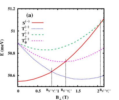
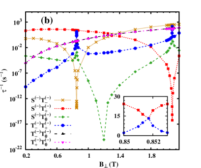
Figure 2: (Color online) (a) The lowest four energy levels vs. perpendicular magnetic field $B_{\perp}$ in a single QD. The anticrossing/crossing points are labeled as $B_{\rm S^{(-)}T_{-}^{(-)}}$, $B_{\rm S^{(-)}T_{0}^{(-)}}$ and $B_{\rm S^{(-)}T_{+}^{(-)}}$. (b) Transition rates vs. the magnetic field. The inset zooms the range near $B_{\rm S^{(-)}T_{-}^{(-)}}$ with the rates of channels ${\rm S^{(-)}T_{+}^{(-)}}$ and ${\rm T_{-}^{(-)}T_{+}^{(-)}}$. In the calculation, $2a=4.344$ nm and $d_{0}=29$ nm.

III.2 PERPENDICULAR MAGNETIC FIELD DEPENDENCE

In this part, we turn to the perpendicular magnetic field case and choose SiGe/Si/SiGe QDs without loss of generality. The relative static dielectric constant is $\kappa=11.9$ in this structure.sze We start from the structure with 32 monoatomic layers of silicon along the growth direction of the quantum well as in the parallel magnetic field case, corresponding to a large valley splitting $2|\Delta_{n_{z}}^{1}|=0.83$ meV. With an electric field 30 kV/cm along the growth direction, one obtains the strength of the Rashba SOC induced by this electric field $a_{0}=\mp 6.06$ m/s and that of the IIA term $b_{0}=\mp 30.31$ m/s for the SOC elements between the states with identical valley index “$\mp$”.nestoklon Moreover, a large effective diameter $d_{0}=29$ nm is taken to ensure that the lowest levels are constructed only by the basis functions with valley index “$-$”.

The first four levels in the QD are plotted in Fig. 2(a) as function of the perpendicular magnetic field. They are labeled as $|S^{(-)}\rangle$, $|T_{+}^{(-)}\rangle$ (spin up), $|T_{0}^{(-)}\rangle$ and $|T_{-}^{(-)}\rangle$ (spin down), according to their major components. The shape of the spectrum can be understood from the single-electron spectrum of Eq. (3). For example, the major component of $|S^{(-)}\rangle$, i.e., $|S^{1(-)}\rangle$, is composed by two electrons in $|001-\rangle$ state, hence the magnetic-field dependence of $\epsilon_{S^{(-)}}$ is given by $2E_{001}^{-}$ approximately. Similarly, the magnetic-field dependence of the triplet $|T_{0}^{(-)}\rangle$ ($|T_{\pm}^{(-)}\rangle$) can be described by $E_{001}^{-}+E_{0-11}^{-}$ ($E_{001}^{-}+E_{0-11}^{-}\pm E_{Z}$, with $E_{z}$ representing the Zeeman splitting), because this state mainly contains the triplet basis $|T^{1(-)}_{0}\rangle$ which involves the single-electron functions $|001-\rangle$ and $|0{-1}1-\rangle$. The qualitative analysis still works even with the strong Coulomb interaction. It is shown that the singlet state $|S^{(-)}\rangle$ intersects the three triplet levels with the increase of the magnetic field. Since the crossing and/or anticrossing points show different properties on ST relaxation as discussed above, we now analyze the intersecting points. We still denote the two-electron angular momentum as $L=l_{1}+l_{2}$, but take the spin states $(S,S_{z})$ instead by considering the perpendicular magnetic field. The SOC Hamiltonian can be rewritten asclimente

$$H_{\rm so}=\frac{2ia_{0}}{\hbar}(P^{+}S^{-}-P^{-}S^{+})-\frac{2b_{0}}{\hbar}(P^{+}S^{+}+P^{-}S^{-}),$$ (17)

with the ladder operations $P^{\pm}$ and $S^{\pm}$ changing $L$ and $S_{z}$ by one unit, respectively. Here, $S^{\pm}=S_{x}\pm iS_{y}$. It is clear that a state with $(L,S_{z})$ can couple with the one with $(L\pm 1,S_{z}\mp 1)$ due to the Rashba SOC and the one with $(L\pm 1,S_{z}\pm 1)$ due to the IIA term. Approximately, the quantum numbers $(L,S_{z})$ of $|T_{-}^{(-)}\rangle$ and $|S^{(-)}\rangle$ are $(-1,-1)$ and $(0,0)$, respectively, according to the wave functions of $|T_{-}^{1(-)}\rangle$ and $|S^{1(-)}\rangle$. Therefore, the IIA term couples these states and an anticrossing event occurs at the intersecting point ($B_{\rm S^{(-)}T_{-}^{(-)}}\sim 0.85$ T), where an energy gap pops up ($\sim 0.2$ $\mu$eV). Similarly, the Rashba SOC results in the anticrossing between $|S^{(-)}\rangle$ and $|T_{+}^{(-)}\rangle$ ($B_{\rm S^{(-)}T_{+}^{(-)}}\sim 2.07$ T). The intersecting point between $|S^{(-)}\rangle$ and $|T_{0}^{(-)}\rangle$ ($B_{\rm S^{(-)}T_{0}^{(-)}}\sim 1.2$ T) is simply a crossing point.

The ST relaxation rates together with the transition rates between two triplet states are plotted in Fig. 2(b), which shows that the lifetimes of the excited states are extremely long (about four orders of magnitude longer than the ST relaxation time in GaAs QDshen ) and strongly depend on the strength of the magnetic field. In the vicinities of the crossing and anticrossing points, the transition rates show intriguing features. For example, at the anticrossing point $B_{\rm S^{(-)}T_{-}^{(-)}}$, one finds that all the transition rates except the one between $|T_{+}^{(-)}\rangle$ and $|T_{0}^{(-)}\rangle$ present either a peak or a valley. According to the previous works,climente ; shen the sharp decrease of the transition rate between $|S^{(-)}\rangle$ and $|T_{-}^{(-)}\rangle$ results from the decrease of the emission phonon energy. The origin of the features of other channels can be understood from Fig. 3, which illustrates the major components of the states around $B_{\rm S^{(-)}T_{-}^{(-)}}$, e.g., $|S^{1(-)}\rangle$ (red solid curve), $|T^{1(-)}_{-}\rangle$ (blue dotted one) and $|T^{1(-)}_{+}\rangle$ (green dashed one). One notices that when the magnetic field approaches $B_{\rm S^{(-)}T_{-}^{(-)}}$, the composition of the $|T_{+}^{(-)}\rangle$ as well as $|T_{0}^{(-)}\rangle$ (not shown) is almost invariant, however, the weight of $|S^{1(-)}\rangle$ ($|T_{-}^{1(-)}\rangle$) in $|S^{(-)}\rangle$ significantly decreases (increases) due to the spin-mixing from the SOC. As the component of $|T^{1(-)}_{-}\rangle$ in $|T_{+}^{(-)}\rangle$ is negligibly small, the weight of $|S^{1(-)}\rangle$ dominates the relaxation rate. Therefore, the relaxation rate between $|T_{+}^{(-)}\rangle$ and $|S^{(-)}\rangle$ decreases as shown in the inset of Fig. 2(b). However, the composition of $|T_{-}^{(-)}\rangle$ varies in the opposite way, hence the transition rate between $|T_{+}^{(-)}\rangle$ and $|T_{-}^{(-)}\rangle$ presents a maximum at $B_{\rm S^{(-)}T_{-}^{(-)}}$. The similar feature of the channel involving $|T_{0}^{(-)}\rangle$ can be interpreted in the same way. Near the anticrossing point $B_{\rm S^{(-)}T_{+}^{(-)}}$, the physics is quite similar and the transition rates of all the channels except one from $|T_{0}^{(-)}\rangle$ to $|T_{-}^{(-)}\rangle$ present either a peak or a valley. However, in the vicinity of the crossing point $B_{\rm S^{(-)}T_{0}^{(-)}}$, only the transition rate between $|S^{(-)}\rangle$ and $|T_{0}^{(-)}\rangle$ shows a sharp decrease due to small phonon energy and other transition rates change slightly, because there is no coupling between $|S^{(-)}\rangle$ and $|T_{0}^{(-)}\rangle$ and the components of all the states remain almost unchanged. The variation of the transition rates far way from the intersecting points can be understood from the dependence of the transition rate on the phonon energy as mentioned in the previous subsection.climente ; shen

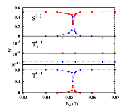
Figure 3: (Color online) Weights of the major components in eigenstates, $W$ [$=|\langle\xi_{0}|\xi\rangle|^{2}$ with $|\xi\rangle=|S^{(-)}\rangle$, $|T_{+}^{(-)}\rangle$, $|T_{-}^{(-)}\rangle$, and $|\xi_{0}\rangle=|S^{1(-)}\rangle$ (red solid curve), $|T_{+}^{1(-)}\rangle$ (green dashed curve), $|T_{-}^{1(-)}\rangle$ (blue dotted curve)], vs. the magnetic field near the anticrossing point $B_{\rm S^{(-)}T_{-}^{(-)}}$.

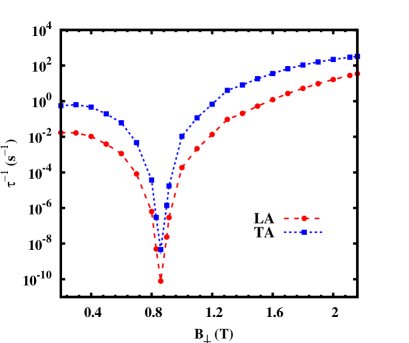
Figure 4: (Color online) Contributions of the LA and TA phonon modes to the relaxation rate between $|T_{-}^{(-)}\rangle$ and $|S^{(-)}\rangle$. The red dashed and blue dotted curves are for the LA and TA modes, respectively. Here, $2a=4.344$ nm and $d_{0}=29$ nm.

To indicate the relative contribution of the LA phonon mode to the ST relaxation, we remove the TA mode from the calculation, vice versa. The magnetic-field dependence of the relaxation rate of the channel between $|T_{-}^{(-)}\rangle$ and $|S^{(-)}\rangle$ is plotted in Fig. 4. One notices that the relaxation rate of the TA mode is always larger than that of the LA mode. Actually, the calculation of the other channels (not shown) also reveals similar conclusion. The reason lies in the different sound velocities of the LA and TA phonons. Since the longitudinal sound velocity is about twice as large as the transverse one,pop the momentum of the LA phonon emission is smaller for a fixed phonon energy. As a result, the transition rate due to the LA phonon emission process is smaller according to Eq. (15).

In addition, we investigate the influence of the effective diameter $d_{0}$ on the ST relaxation. The results are plotted in Fig. 5. One notices that the behavior of the transition rates is similar to what obtained above by changing the perpendicular magnetic field. Here, an anticrossing point between the singlet and one of the triplets ($|T_{-}^{(-)}\rangle$) is also observed at $d_{0}\sim 27.4$ nm. In the vicinity of this point, we also find the relaxation rate between $|T_{-}^{(-)}\rangle$ and $|S^{(-)}\rangle$ is strongly suppressed and the rates of other transition channels relevant to these two states show a rapid increase or decrease too. Therefore, the manipulation of the ST relaxation by tuning the dot size is also feasible. In the experiment, the dot size can be controlled electrically.shaji

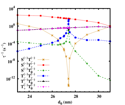
Figure 5: (Color online) Transition rates vs. effective dot diameter $d_{0}$. In the calculation, $2a=4.344$ nm and $B_{\perp}=1$ T.

Finally, we also study the case of small valley splitting by taking 27 monoatomic layers along the growth direction of the quantum well, where $2|\Delta_{n_{z}}^{1}|=0.35$ meV according to Eq. (8). In this configuration, the SOC strengths are unavailable in the literature. We extract these parameters according to the results of odd monoatomic layers calculated by Nestoklon et al.nestoklon and obtain $a_{0}=\mp 2.28$ m/s and $b_{0}=\pm 37.93$ m/s for the SOC elements between the states with identical valley indices “$\mp$”, when the same electric field ($30$ kV/cm) as the case of large valley splitting is applied. One finds that the lowest triplet states (denoted as $|T_{-}^{(m)}\rangle$, $|T_{0}^{(m)}\rangle$, and $|T_{+}^{(m)}\rangle$) are mainly constructed by the single-electron functions $|001-\rangle$ and $|001+\rangle$, in a QD with the effective diameter 18 nm under a low magnetic field. However, the major component of the lowest singlet ($|S^{(-)}\rangle$) remains in the same configuration as the case of large valley splitting. Interestingly, the second singlet level ($|S^{\ast(m)}\rangle$), whose major component is constructed by the single-electron basis functions $|001-\rangle$ and $|001+\rangle$, is almost degenerate with $|T_{0}^{(m)}\rangle$, which reveals that the intervalley Coulomb exchange interaction is rather small.li In this case, no anticrossing point is observed between the relevant states, because of the absence of the SOC element between different valley states when only the lowest subband is relevant, as mentioned above. Moreover, we find that the relaxations from the three triplet states to $|S^{(-)}\rangle$ are much slower than those in the case of large valley splitting because these triplets and $|S^{(-)}\rangle$ are in different sets as mentioned above.

IV SUMMARY

In summary, we have investigated the ST relaxation in silicon QDs with magnetic fields in either the Voigt or the Faraday configuration. Our results in the Voigt configuration agree pretty well with the recent experiment in Si/SiO₂ QDs. We have identified that the origin of the relaxation channel in the experiment is between the lowest singlet and triplet in the set with single valley eigenstate “$-/+$” (more likely the “$-$” one). Besides, we also predict the enhancement of the ST relaxation process in the vicinity of the anticrossing point due to the SOCs when the magnetic field further increases, which should be checked by future experiments. We then focus on the ST relaxation in the Faraday configuration in SiGe/Si/SiGe QDs and discuss the role of the valley splittings. In the case of large valley splitting, the lowest levels are all constructed by the eigenstates from the lowest valley state. We find that the transition rates are about four orders of magnitude smaller than those of GaAs QDs due to the weak SOC in silicon. The transition rates can be effectively manipulated by tuning the magnetic field and dot size. From the magnetic-field and dot-size dependence of energy levels, we also observe ST crossing/anticrossing points. In the vicinity of the anticrossing point, there exists a small energy gap between the singlet and one of the triplet states due to the SOC. The transition rates of the channels relevant to these two states show a sharp increase or decrease. We show that the contribution of the TA phonon mode is larger than that of the LA one due to the smaller transverse sound velocity. As for the small valley splitting, the eigenstates from both valley states contribute. We find the ST relaxation rates in this case are much smaller.

Appendix A G IN COULOMB INTERACTION

$G$ in Eq. (12) is given by

$$G(\phi_{n_{1}l_{1}n_{z1}}^{\gamma_{1}},\phi_{n_{2}l_{2}n_{z2}}^{\gamma_{2}},\phi_{n_{1}^{\prime}l_{1}^{\prime}n_{z1}^{\prime}}^{\gamma_{1}^{\prime}},\phi_{n_{2}^{\prime}l_{2}^{\prime}n_{z2}^{\prime}}^{\gamma_{2}^{\prime}})=\int_{0}^{\infty}dk_{\|}\int_{-\infty}^{\infty}dk_{z}k_{\|}P_{n_{1}l_{1}}^{n_{1}^{\prime}l_{1}^{\prime}}(k_{\|})P^{n_{2}l_{2}}_{n_{2}^{\prime}l_{2}^{\prime}}(k_{\|})\frac{W_{n_{z1}\gamma_{1}}^{n_{z1}^{\prime}\gamma_{1}^{\prime}}(k_{z})(W^{n_{z2}\gamma_{2}}_{n_{z2}^{\prime}\gamma_{2}^{\prime}}(k_{z}))^{\ast}}{k^{2}},$$ (18)

where $P_{nl}^{n^{\prime}l^{\prime}}$ and $W_{n_{z}\gamma}^{n_{z}^{\prime}\gamma^{\prime}}$ come from the lateral and vertical parts of the matrix element $\langle n,l,n_{z},\gamma|e^{i{\bf k}\cdot{\bf r}}|n^{\prime},l^{\prime},n_{z}^{\prime},\gamma^{\prime}\rangle$, respectively. $P$ ischeng

$$P_{nl}^{n^{\prime}l^{\prime}}(k_{\|})=\sqrt{\frac{n!n^{\prime}!}{(n+|l|)!(n^{\prime}+|l^{\prime}|)!}}{\rm exp}(-\frac{k_{\|}^{2}}{4\alpha^{2}})\sum_{i=0}^{n^{\prime}}\sum_{j=0}^{n}C_{n^{\prime},|l^{\prime}|}^{i}C_{n,|l|}^{j}\bar{n}!L_{\bar{n}}^{|l-l^{\prime}|}(\frac{k_{\|}^{2}}{4\alpha^{2}})\Big{[}{\rm sgn}(l^{\prime}-l)\frac{k_{\|}}{2\alpha}\Big{]}^{|l^{\prime}-l|},$$ (19)

with $C_{n,l}^{i}=\frac{(-1)^{i}}{i!}{n+l\choose n-i}$ and $\bar{n}=i+j+(|l|+|l^{\prime}|-|l^{\prime}-l|)/2$. sgn $(x)$ represents the sign function and $W$ reads $W_{n_{z}\gamma}^{n_{z}^{\prime}\gamma^{\prime}}=\langle n_{z},\gamma|{\rm exp}(ik_{z}z)|n_{z}^{\prime},\gamma^{\prime}\rangle$.

References

- (1) D. Loss and D. P. DiVincenzo, Phys. Rev. A 57, 120 (1998).
- (2) F. H. L. Koppens, C. Buizert, K.-J. Tielrooij, I. T. Vink, K. C. Nowack, T. Meunier, L. P. Kouwenhoven, and L. M. K. Vandersypen, Nature (London) 442, 766 (2006).
- (3) J. R. Petta, A. C. Johnson, J. M. Taylor, E. A. Laird, A. Yacoby, M. D. Lukin, C. M. Marcus, M. P. Hanson, and A. C. Gossard, Science 309, 2180 (2005).
- (4) F. H. L. Koppens, J. A. Folk, J. M. Elzerman, R. Hanson, L. H. Willems van Beveren, I. T. Vink, H. P. Tranitz, W. Wegscheider, L. P. Kouwenhoven, and L. M. K. Vandersypen, Science 309, 1346 (2005).
- (5) J. R. Petta, A. C. Johnson, A. Yacoby, C. M. Marcus, M. P. Hanson, and A. C. Gossard, Phys. Rev. B 72, 161301(R) (2005).
- (6) S. Sasaki, T. Fujisawa, T. Hayashi, and Y. Hirayama, Phys. Rev. Lett. 95, 056803 (2005).
- (7) T. Meunier, I. T. Vink, L. H. Willems van Beveren, K.-J. Tielrooij, R. Hanson, F. H. L. Koppens, H. P. Tranitz, W. Wegscheider, L. P. Kouwenhoven, and L. M. K. Vandersypen, Phys. Rev. Lett. 98, 126601 (2007).
- (8) J. L. Cheng, M. W. Wu, and C. Lü, Phys. Rev. B 69, 115318 (2004).
- (9) K. Shen and M. W. Wu, Phys. Rev. B 76, 235313 (2007).
- (10) J. H. Jiang, Y. Y. Wang, and M. W. Wu, Phys. Rev. B 77, 035323 (2008).
- (11) V. N. Golovach, A. Khaetskii, and D. Loss, Phys. Rev. B 77, 045328 (2008).
- (12) J. M. Taylor, H.-A. Engel, W. Dür, A. Yacoby, C. M. Marcus, P. Zoller, and M. D. Lukin, Nature Phys. 1, 177 (2005).
- (13) J. M. Taylor, J. R. Petta, A. C. Johnson, A. Yacoby, C. M. Marcus, and M. D. Lukin, Phys. Rev. B 76, 035315 (2007).
- (14) R. Hanson, L. P. Kouwenhoven, J. R. Petta, S. Tarucha, and L. M. K. Vandersypen, Rev. Mod. Phys. 79, 1217 (2007).
- (15) R. Hanson, B. Witkamp, L. M. K. Vandersypen, L. H. Willems van Beveren, J. M. Elzerman, and L. P. Kouwenhoven, Phys. Rev. Lett. 91, 196802 (2003).
- (16) S. Amasha, K. MacLean, I. Radu, D. M. Zumbühl, M. A. Kastner, M. P. Hanson, and A. C. Gossard, arXiv:0607110.
- (17) J. I. Climente, A. Bertoni, G. Goldoni, M. Rontani, and E. Molinari, Phys. Rev. B 75, 081303(R) (2007).
- (18) D. Paget, G. Lampel, B. Sapoval, and V. I. Safarov. Phys. Rev. B 15, 5780 (1977).
- (19) G. E. Pikus and A. N. Titkov, Optical Orientation (Berlin, Springer, 1984).
- (20) S. I. Erlingsson, Y. V. Nazarov, and V. I. Fal’ko, Phys. Rev. B 64, 195306 (2001).
- (21) A. Khaetskii, D. Loss, and L. Glazman, Phys. Rev. B 67, 195329 (2003).
- (22) W. M. Witzel and S. D. Sarma, Phys. Rev. B 74, 035322 (2006).
- (23) W. Yao, R.-B. Liu, and L. J. Sham, Phys. Rev. B 74, 195301 (2006).
- (24) W. Zhang, V. V. Dobrovitski, K. A. Al-Hassanieh, E. Dagotto, and B. N. Harmon, Phys. Rev. B 74, 205313 (2006).
- (25) C. Deng and X. Hu, Phys. Rev. B 78, 245301 (2008).
- (26) W. A. Coish, J. Fischer, and D. Loss, Phys. Rev. B 77, 125329 (2008).
- (27) L. Cywiński, W. M. Witzel, and S. D. Sarma, Phys. Rev. Lett. 102, 057601 (2009).
- (28) L. Cywiński, W. M. Witzel, and S. D. Sarma, Phys. Rev. B 79, 245314 (2009).
- (29) G. Dresselhaus, Phys. Rev. 100, 580 (1955).
- (30) E. I. Rashba, Fiz. Tverd. Tela (Leningrad) 2, 1224 (1960) [Sov. Phys. Solid State 2, 1109 (1960)].
- (31) D. Culcer, L. Cywiński, Q. Li, X. Hu, and S. D. Sarma, Phys. Rev. B 80, 205302 (2009).
- (32) Q. Li, L. Cywiński, D. Culcer, X. Hu, and S. D. Sarma, Phys. Rev. B 81, 085313 (2010).
- (33) M. Prada. R. H. Blick, and R. Joynt, Phys. Rev. B 77, 115438 (2008).
- (34) W. Pan, X. Z. Yu, and W. Z. Shen, Appl. Phys. Lett. 95, 013103 (2009).
- (35) H. W. Liu, T. Fujisawa, Y. Ono, H. Inokawa, A. Fujiwara, K. Takashina, and Y. Hirayama, Phys. Rev. B 77, 073310 (2008).
- (36) N. Shaji, C. B. Simmons, M. Thalakulam, L. J. Klein, H. Qin, H. Luo, D. E. Savage, M. G. Lagally, A. J. Rimberg, R. Joynt, M. Friesen, R. H. Blick, S. N. Coppersmith, and M. A. Eriksson, Nature Phys. 4, 540 (2008).
- (37) D. Culcer, L. Cywiński, Q. Li, X. Hu, and S. D. Sarma, arXiv:1001.5040.
- (38) M. Xiao, M. G. House, and H. W. Jiang, Phys. Rev. Lett. 104, 096801 (2010).
- (39) W. A. Coish and D. Loss, Phys. Rev. B 70, 195340 (2004).
- (40) J. M. Taylor, W. Dür, P. Zoller, A. Yacoby, C. M. Marcus, and M. D. Lukin, Phys. Rev. Lett. 94, 236803 (2005).
- (41) L. Vervoort, R. Ferreira, and P. Voisin, Phys. Rev. B 56, R12744 (1997).
- (42) L. Vervoort, R. Ferreira, and P. Voisin, Semicond. Sci. Technol. 14, 227 (1999).
- (43) M. O. Nestoklon, E. L. Ivchenko, J.-M. Jancu, and P. Voisin, Phys. Rev. B 77, 155328 (2008).
- (44) T. B. Boykin, G. Klimeck, M. A. Eriksson, M. Friesen, S. N. Coppersmith, P. von Allmen, F. Oyafuso, and S. Lee, Appl. Phys. Lett. 84, 115 (2004).
- (45) M. Friesen, S. Chutia, C. Tahan, and S. N. Coppersmith, Phys. Rev. B 75, 115318 (2007).
- (46) V. Fock, Z. Phys. 47, 446 (1928).
- (47) C. G. Darwin, Proc. Cambrige Philos. Soc. 27, 86 (1931).
- (48) A. L. Saraiva, M. J. Calderón, X. Hu, S. D. Sarma, and B. Koiller, Phys. Rev. B 80, 081305(R) (2009).
- (49) S. Chutia, S. N. Coppersmith, and M. Friesen, Phys. Rev. B 77, 193311 (2008).
- (50) E. Pop, R. W. Dutton, and K. E. Goodson, J. Appl. Phys. 96, 4998 (2004).
- (51) E. Sonder and D. K. Stevens, Phys. Rev. 110, 1027 (1958).
- (52) R. N. Dexter, B. Lax, A. F. Kip, and G. Dresselhaus, Phys. Rev. 96, 222 (1954).
- (53) C. F. O. Graeff, M. S. Brandt, M. Stutzmann, M. Holzmann, G. Abstreiter, and F. Schäffler, Phys. Rev. B 59, 13242 (1999).
- (54) S. M. Sze, Physics of Semiconductor Devices (Wiley-Interscience, New York, 1981), p. 849.