Difficulties in analytic computation for relative entropy of entanglement

Abstract

It is known that relative entropy of entanglement for an entangled state $\rho$ is defined via its closest separable (or positive partial transpose) state $\sigma$. Recently, it has been shown how to find $\rho$ provided that $\sigma$ is given in two-qubit system. In this paper we study on the reverse process-i.e., how to find $\sigma$ provided that $\rho$ is given. It is shown that if $\rho$ is one of Bell-diagonal, generalized Vedral-Plenio, and generalized Horodecki states, one can find $\sigma$ from a geometrical point of view. This is possible due to the following two facts: (i) The Bloch vectors of $\rho$ and $\sigma$ are identical with each other (ii) The correlation vector of $\sigma$ can be computed from a crossing point between a minimal geometrical object, in which all separable states reside in the presence of Bloch vectors, and a straight line, which connects the point corresponding to the correlation vector of $\rho$ and the nearest vertex of the maximal tetrahedron, where all two-qubit states reside. It is shown, however, that these nice properties are not maintained for the arbitrary two-qubit states.

I Introduction

It is well known that entanglement of quantum states is an important physical resource in the context of the quantum information theories. It plays a crucial role in quantum teleportationbennett93 , superdense codingbennett92 , quantum cloningscarani05 , quantum cryptographyekert91 and quantum computer technologyvidal03-1 ; nielsen00 . Therefore, to understand how to quantify and how to characterize the entanglement for a given quantum state is an highly important physical task.

Many entanglement measures have been developed for last few years. Above all, in our opinion, the most important entanglement measure is a distillable entanglementbennett96 , which quantifies how many maximally entangled states can be constructed from the copies of the given quantum state in the asymptotic region. The importance of the distillable entanglement arises due to the fact that the entanglement is fragile when noises interfere the quantum information processing. The disadvantage of the distillable entanglement is its calculational difficulty. In order to compute the distillable entanglement analytically we should find the optimal purification (or distillation) protocol. If this optimal protocol generates $n$ maximally entangled states from $m$-copies of the quantum state $\rho$, the distillable entanglement for $\rho$ is given by

$$D(\rho)=\lim_{m\rightarrow\infty}\frac{n}{m}.$$ (1)

However, finding an optimal purification protocol is an highly non-trivial task. It makes it difficult to compute the distillable entanglement analytically.

Fortunately, the tight upper bound of the distillable entanglement has been developed in Ref.vedral-97-1 ; vedral-97-2 . In these references the new entanglement measure called relative entropy of entanglement (REE) was introduced. It is defined as

$$E_{R}(\rho)=\min_{\sigma\in{\cal D}}S(\rho||\sigma),$$ (2)

where ${\cal D}$ is a set of separable states and $S(\rho||\sigma)$ is a quantum relative entropy-i.e., $S(\rho||\sigma)=\mbox{tr}(\rho\ln\rho-\rho\ln\sigma)$. It was shown in Ref.vedral-97-2 that $E_{R}(\rho)$ is a upper bound of the distillable entanglement. Subsequently, Rainsrains-99-1 ; rains-99-2 has shown that

$$\tilde{E}_{R}(\rho)=\min_{\sigma\in{\cal D}_{PPT}}S(\rho||\sigma),$$ (3)

where ${\cal D}_{PPT}$ is a set of positive partial transposition (PPT) states, is more tight upper bound when $\rho$ is an higher-dimensional bipartite state. Using the facts that the REE is an upper bound of the distillable entanglement and Smolin statesmolin00 is a bound entangled state, the distillable entanglement for the various Bell-state mixtures has been analytically computedghosh01 ; chen02 ; chen03 . In order to understand the distillable entanglement more deeply, therefore, it is important to develop the various techniques for the explicit computation of the REE. Of course, regardless of the distillable entanglement, the development of the calculation technique for the REE itself is important to understand the characterization of entanglement more profoundly. For last few years many properties of the REE were investigatedhoro-07-1 . Furthermore, recently relation between the REE and other distance measures has been studiedhayashi05 ; wei08 .

In this paper we confine ourselves to the REE when $\rho$ is two-qubit states-i.e., $\rho\in{\cal H}^{2}\otimes{\cal H}^{2}$. Since there is no bound-entangled state in this case, $E_{R}(\rho)$ and $\tilde{E}_{R}(\rho)$ defined in Eq.(2) and Eq.(3) are same. Let $\sigma^{*}$ be the closest separable state (CSS) of $\rho$. Then, $E_{R}(\rho)$ is given by

$$E_{R}(\rho)=\min_{\sigma\in{\cal D}}S(\rho||\sigma)=S(\rho||\sigma^{*}).$$ (4)

When the CSS $\sigma^{*}$ is explicitly given and it is full rank, Ref.miran-08-1 has presented how to construct the set of the entangled states, whose CSS are $\sigma^{*}$. Let $\lvert i\rangle$ and $\lambda_{i}$ be eigenvectors and corresponding eigenvalues of $\sigma^{*}$. If $\sigma^{*}$ is the CSS (hence, edge) state, then its partial transposition $\sigma^{\Gamma}$ is rank deficient. Let $\lvert\phi\rangle$ be the kernel of $\sigma^{\Gamma}$-i.e.,

$$\sigma^{\Gamma}\lvert\phi\rangle=0.$$ (5)

Then, the set of the entangled states $\rho(x)$, whose CSS are $\sigma^{*}$, is given by the following one-parameter family expression:

$$\rho(x)=\sigma^{*}-xG(\sigma^{*})$$ (6)

$$G(\sigma^{*})=\sum_{i,j}G_{ij}\lvert i\rangle\langle i\lvert(\lvert\phi\rangle\langle\phi\lvert)^{\Gamma}\lvert j\rangle\langle j\lvert,$$

where $x\geq 0$ and

$$G_{ij}=\left\{\begin{array}[]{cc}\lambda_{i}&\hskip 14.22636pt\mbox{for}\hskip 5.69046pti=j\\ \frac{\lambda_{i}-\lambda_{j}}{\ln\lambda_{i}-\ln\lambda_{j}}&\hskip 14.22636pt\mbox{for}\hskip 5.69046pti\neq j.\end{array}\right.$$ (9)

When, however, the entangled state $\rho$ is explicitly given, it is difficult to use Eq.(6) for finding its CSS. In other words we have to find the reverse process of Ref.miran-08-1 in order to derive the closed formula of the REE for the arbitrary two-qubit state $\rho$ as Wootterswoot-98 has done in the entanglement of formation. Unfortunately, still it is an unsolved problemopen05 .

In this paper we will explore the reverse process of Ref.miran-08-1 . We will show that the reverse process of Ref.miran-08-1 is possible, at least, for the Bell-diagonal, generalized Vedral-Plenio, and generalized Horodecki states. We present a method for finding the corresponding CSS systematically for these states by generalizing the geometrical method discussed by Horodecki in Ref.horo-96-1 . We also discuss why it is difficult to find the CSS for the arbitrary two-qubit mixed states from the geometrical point of view. The paper is organized as follows. In section II we will show how to find the CSS for the Bell-diagonal states. In section III we discuss how the geometrical objects presented in Ref.horo-96-1 such as tetrahedron ${\cal T}$ and octahedron ${\cal L}$ are deformed in the presence of the non-zero Bloch vectors. In section IV and section V we present a method for finding the corresponding CSS for the generalized Vedral-Plenio and generalized Horodecki states, respectively. In section VI we discuss why it is very difficult task to find the CSS for the arbitrary two-qubit states from the geometrical point of view. In section VII a brief conclusion is given.

II CSS for the Bell-Diagonal States

In this section we show how to find the CSS when $\rho$ is the Bell-diagonal state from the geometrical point of view. In fact, this problem was already solved in Ref.vedral-97-2 long ago. The reason why we re-consider the same problem is to stress the geometrical analysis.

An arbitrary two-qubit state can be represented as follows:

$$\rho=\frac{1}{4}\left[I\otimes I+{\bm{r}}\cdot{\bm{\sigma}}\otimes I+I\otimes{\bm{s}}\cdot{\bm{\sigma}}+\sum_{m,n=1}^{3}g_{mn}\sigma_{m}\otimes\sigma_{n}\right],$$ (10)

where ${\bm{r}}$ and ${\bm{s}}$ are Bloch vectors and $\sigma_{i}$ is usual Pauli matrix. The coefficients $g_{mn}$ form a real matrix and represent the interaction of the qubits. If state $\rho$ is explicitly given, one can derive the Bloch vectors ${\bm{r}}$ and ${\bm{s}}$ and the correlation tensor $g_{ij}$ as follows:

$${\bm{r}}=\mbox{tr}(\rho_{A}{\bm{\sigma}}),\hskip 28.45274pt{\bm{s}}=\mbox{tr}(\rho_{B}{\bm{\sigma}}),\hskip 28.45274ptg_{ij}=\mbox{tr}(\rho\sigma_{i}\otimes\sigma_{j}),$$ (11)

where $\rho_{A}=\mbox{tr}_{B}\rho$ and $\rho_{B}=\mbox{tr}_{A}\rho$. It is well known that an appropriate local unitary (LU) transformation of $\rho$ can make $g_{mn}$ to be diagonal (see appendix of Ref.jung-08-1 ). Since entanglement is invariant under the LU transformation, it is in general sufficient to consider the case of diagonal $g_{mn}$ for the discussion of entanglement. Thus, without loss of generality, one can express $\rho$ as

$$\rho=\frac{1}{4}\left[I\otimes I+{\bm{r}}\cdot{\bm{\sigma}}\otimes I+I\otimes{\bm{s}}\cdot{\bm{\sigma}}+\sum_{n=1}^{3}g_{n}\sigma_{n}\otimes\sigma_{n}\right].$$ (12)

If $\rho=\lvert\beta_{i}\rangle\langle\beta_{i}\lvert$, where

$$\lvert\beta_{1}\rangle=\frac{1}{\sqrt{2}}\left(\lvert 00\rangle+\lvert 11\rangle\right)\hskip 56.9055pt\lvert\beta_{2}\rangle=\frac{1}{\sqrt{2}}\left(\lvert 00\rangle-\lvert 11\rangle\right)$$ (13)

$$\lvert\beta_{3}\rangle=\frac{1}{\sqrt{2}}\left(\lvert 01\rangle+\lvert 10\rangle\right)\hskip 56.9055pt\lvert\beta_{4}\rangle=\frac{1}{\sqrt{2}}\left(\lvert 01\rangle-\lvert 10\rangle\right),$$

it is easy to show that the corresponding Bloch vectors ${\bm{r}}$ and ${\bm{s}}$ are vanishing and the corresponding correlation tensor $g_{mn}$ become

$$g_{1}=\mbox{diag}(1,-1,1)\hskip 14.22636ptg_{2}=\mbox{diag}(-1,1,1)\hskip 14.22636ptg_{3}=\mbox{diag}(1,1,-1)\hskip 14.22636ptg_{4}=\mbox{diag}(-1,-1,-1).$$ (14)

If, therefore, $\rho$ is Bell-diagonal state, the Bloch vectors ${\bm{r}}$ and ${\bm{s}}$ are always null vectors.

Since we are considering on the diagonal case of the correlation tensor, we will regard, from now on, the tensor as a vector, whose components are equal to the diagonal elements. When ${\bm{r}}={\bm{s}}=0$, Horodecki has shown in Ref.horo-96-1 that the total two-qubit states belong to the tetrahedron ${\cal T}$ with vertices $v_{1}=(1,-1,1)$, $v_{2}=(-1,1,1)$, $v_{3}=(1,1,-1)$ and $v_{4}=(-1,-1,-1)$ in the correlation vector space. Ref.horo-96-1 also has shown that the separable states (with ${\bm{r}}={\bm{s}}=0$) belong to the octahedron ${\cal L}$ with vertices $o_{1}^{(\pm)}=(\pm 1,0,0)$, $o_{2}^{(\pm)}=(0,\pm 1,0)$ and $o_{3}^{(\pm)}=(0,0,\pm 1)$. This is pictorially represented in Fig. 1.

Figure 1: The total Bell-diagonal states belong to the tetrahedron $(v_{1},v_{2},v_{3},v_{4})$ and the set of the separable states belong to the octahedron, whose vertices are $o_{1}^{\pm}$, $o_{2}^{\pm}$ and $o_{3}^{\pm}$. As this figure shows, the planes $(o_{1}^{(+)},o_{2}^{(-)},o_{3}^{(-)})$, $(o_{1}^{(+)},o_{2}^{(+)},o_{3}^{(+)})$, $(o_{1}^{(-)},o_{2}^{(-)},o_{3}^{(+)})$ and $(o_{1}^{(-)},o_{2}^{(+)},o_{3}^{(-)})$ are contained in the planes $(v_{1},v_{3},v_{4})$, $(v_{1},v_{2},v_{3})$, $(v_{1},v_{2},v_{4})$ and $(v_{2},v_{3},v_{4})$, respectively. Therefore, all entangled Bell-diagonal mixtures belong to the small four tetrahedra $(v_{1},o_{1}^{(+)},o_{2}^{(-)},o_{3}^{(+)})$, $(v_{2},o_{1}^{(-)},o_{2}^{(+)},o_{3}^{(+)})$, $(v_{3},o_{1}^{(+)},o_{2}^{(+)},o_{3}^{(-)})$ and $(v_{4},o_{1}^{(-)},o_{2}^{(-)},o_{3}^{(-)})$.

As Fig. 1 shows, the planes $(o_{1}^{(+)},o_{2}^{(-)},o_{3}^{(-)})$, $(o_{1}^{(+)},o_{2}^{(+)},o_{3}^{(+)})$, $(o_{1}^{(-)},o_{2}^{(-)},o_{3}^{(+)})$ and $(o_{1}^{(-)},o_{2}^{(+)},o_{3}^{(-)})$ are parts of the planes $(v_{1},v_{3},v_{4})$, $(v_{1},v_{2},v_{3})$, $(v_{1},v_{2},v_{4})$ and $(v_{2},v_{3},v_{4})$ ,respectively. Therefore, all entangled Bell-diagonal mixtures belong to the small four tetrahedra $(v_{1},o_{1}^{(+)},o_{2}^{(-)},o_{3}^{(+)})$, $(v_{2},o_{1}^{(-)},o_{2}^{(+)},o_{3}^{(+)})$, $(v_{3},o_{1}^{(+)},o_{2}^{(+)},o_{3}^{(-)})$ and $(v_{4},o_{1}^{(-)},o_{2}^{(-)},o_{3}^{(-)})$.

Now, we show how to perform the reverse process of Ref.miran-08-1 when $\rho$ is an entangled Bell-diagonal state. This can be achieved by following two theorems.

Theorem 1. Every Bell state has infinite CSS, which cover fully the nearest surface of the octahedron ${\cal L}$.

Proof. It is sufficient to prove this theorem when $\rho=\lvert\beta_{1}\rangle\langle\beta_{1}\lvert$. When $\rho=\lvert\beta_{i}\rangle\langle\beta_{i}\lvert\hskip 2.84544pt(i=2,3,4)$, one can prove the theorem similarly.

Let $\sigma$ be a following Bell-diagonal state:

$$\sigma=\frac{1}{4}\left[I\otimes I+\sum_{n=1}^{3}p_{n}\sigma_{n}\otimes\sigma_{n}\right]$$ (15)

with ${\bm{p}}=(x,y,z)$. Then, it is easy to show that the spectral decomposition of $\sigma$ is

$$\sigma=\frac{1+x-y+z}{4}\lvert\beta_{1}\rangle\langle\beta_{1}\lvert+\frac{1-x+y+z}{4}\lvert\beta_{2}\rangle\langle\beta_{2}\lvert$$ (16)

$$\hskip 19.91684pt+\frac{1+x+y-z}{4}\lvert\beta_{3}\rangle\langle\beta_{3}\lvert+\frac{1-x-y-z}{4}\lvert\beta_{4}\rangle\langle\beta_{4}\lvert.$$

The nearest surface of ${\cal L}$ from $\rho=\lvert\beta_{1}\rangle\langle\beta_{1}\lvert$ is $(o_{1}^{(+)},o_{2}^{(-)},o_{3}^{(+)})$, whose surface equation is $x-y+z=1$. If $\sigma$ belongs to the surface $(o_{1}^{(+)},o_{2}^{(-)},o_{3}^{(+)})$, it is easy to show that $S(\rho||\sigma)=\ln 2$, which exactly coincides with the REE of the Bell statesvedral-97-1 . Therefore, $\sigma$ on the surface $(o_{1}^{(+)},o_{2}^{(-)},o_{3}^{(+)})$ is the CSS of $\lvert\beta_{1}\rangle\langle\beta_{1}\lvert$.

Now, let us consider the case where $\sigma$ belongs to other surface. For example, let us assume that $\sigma$ belongs to the surface $(o_{1}^{(+)},o_{2}^{(+)},o_{3}^{(-)})$, whose surface equation is $x+y-z=1$. Then, $S(\rho||\sigma)$ reduces to $\ln 2-\ln x$, which is less than $\ln 2$ if $x\neq 1$. Therefore $\sigma$ on $(o_{1}^{(+)},o_{2}^{(+)},o_{3}^{(-)})$ is not CSS of $\lvert\beta_{1}\rangle\langle\beta_{1}\lvert$. By same way one can show that $\sigma$ on $(o_{1}^{(-)},o_{2}^{(+)},o_{3}^{(+)})$ or $(o_{1}^{(-)},o_{2}^{(-)},o_{3}^{(-)})$ is not CSS of $\lvert\beta_{1}\rangle\langle\beta_{1}\lvert$, which completes the proof.

Theorem 2. The CSS of the any Bell-diagonal state $\rho$ corresponds to the crossing point between the nearest surface of ${\cal L}$ from $\rho$ and the straight line $\ell$, which connects $\rho$ and the nearest vertex of ${\cal T}$ from $\rho$.

Proof. If $\sigma$ is CSS of $\rho$, the CSS of $\tilde{\rho}=x\rho+(1-x)\sigma$ is also $\sigma$vedral-97-2 . Let $\rho$ be $\rho=\lvert\beta_{1}\rangle\langle\beta_{1}\lvert$. Then, theorem 1 implies that $\sigma$ can be any point on the surface $(o_{1}^{(+)},o_{2}^{(-)},o_{3}^{(+)})$. Let $\tilde{\rho}$ belong to the small tetrahedron $(v_{1},o_{1}^{(+)},o_{2}^{(-)},o_{3}^{(+)})$. Note that $\tilde{\rho}$ corresponds to a internally dividing point of the line segment $\overline{\rho\sigma}$. Since Eq.(6) implies that the set of the entangled states which have same CSS should be represented by the straight line, the only possible $\sigma$ as CSS of $\tilde{\rho}$ is a crossing point between a line $\overline{\rho\tilde{\rho}}$ and the surface $(o_{1}^{(+)},o_{2}^{(-)},o_{3}^{(+)})$, which completes the proof for the Bell-diagonal states.

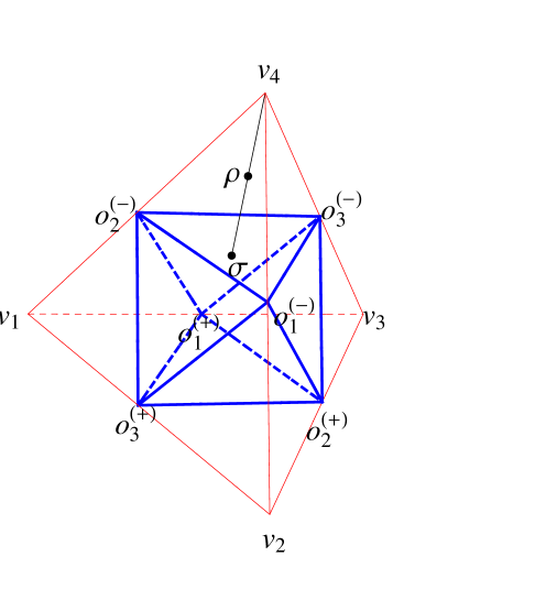
Figure 2: This figure shows how to find the CSS for the Bell-diagonal state. First, extend the line segment between $\rho$ and the point corresponding to the nearest vertex of ${\cal T}$. Second, compute the coordinate of the crossing point between the line and the nearest surface of the octahedron ${\cal L}$. Finally, find the CSS of $\rho$ which corresponds to the crossing point.

By making use of the Theorem 2 one can always find the CSS $\sigma$ if $\rho$ is a Bell-diagonal state. Fig. 2 shows how to find the CSS for the Bell-diagonal state. First, extend the line segment between $\rho$ and the point corresponding to the nearest vertex of ${\cal T}$. Second, compute the coordinate of the crossing point between the line and the nearest surface of the octahedron ${\cal L}$. Finally, find the CSS which corresponds to the crossing point. This complete the reverse process of Ref.miran-08-1 .

III Geometrical Deformation of ${\cal T}$ and ${\cal L}$

When the Bloch vectors ${\bm{r}}$ and ${\bm{s}}$ are non-zero, the geometrical objects ${\cal T}$ and ${\cal L}$ should be deformed. In this section we will discuss how ${\cal T}$ and ${\cal L}$ are deformed. In order to perform the following analysis analytically we consider in this paper the case where ${\bm{r}}$ and ${\bm{s}}$ are parallel to each other. It is worthwhile noting that if ${\bm{r}}$ and ${\bm{s}}$ are $x$- or $y$-direction, one can make them to be $z$-directional via the appropriate local-unitary transformation. For example, if they are $x$-direction, $\rho^{\prime}=(U\otimes U)\rho(U\otimes U)^{\dagger}$ with

$$U=\frac{1}{\sqrt{2}}\left(\begin{array}[]{cc}1&1\\ -1&1\end{array}\right)$$

has $z$-directional Bloch vectors and its correlation vector changes from $(g_{1},g_{2},g_{3})$ to $(-g_{3},g_{2},g_{1})$. Similarly, one can change the state with $y$-directional Bloch vectors into the state with $z$-directional Bloch vectors without altering the diagonal property of the correlation term.

In this reason it is reasonable to assume that the directions of the Bloch vectors are $z$-direction by writing ${\bm{r}}=(0,0,r)$ and ${\bm{s}}=(0,0,s)$. In this case the arbitrary two-qubit state $\rho$ defined in Eq.(12) with $\bm{g}=(q_{1},q_{2},q_{3})$ reduces to

$$\rho=\frac{1}{4}\left(\begin{array}[]{cccc}1+r+s+q_{3}&0&0&q_{1}-q_{2}\\ 0&1+r-s-q_{3}&q_{1}+q_{2}&0\\ 0&q_{1}+q_{2}&1-r+s-q_{3}&0\\ q_{1}-q_{2}&0&0&1-r-s+q_{3}\end{array}\right).$$ (21)

Figure 3: The deformation of ${\cal T}$ is plotted when $r=s=0.3$ (Fig. 3a), $r=-s=0.3$ (Fig. 3b), $r=s=0.5$ (Fig. 3c) and $r=-s=0.5$ (Fig. 3d). For comparison we plot ${\cal T}$ together. The appearance of non-zero Bloch vectors generally shrink the tetrahedron. The shrinking rate becomes larger with increasing the norm of the Bloch vectors.

The eigenvalues and eigenvectors of $\rho$ are summarized at Table I.

eigenvalues of $\rho$	eigenvectors of $\rho$
$\mu_{\pm}=\frac{1}{4}\left\{(1-q_{3})\pm M_{1}\right\}$	$\lvert\mu_{\pm}\rangle=\frac{1}{\Lambda_{\pm}}\left[(q_{1}+q_{2})\lvert 01\rangle-\left\{(r-s)\mp M_{1}\right\}\lvert 10\rangle\right]$
$\nu_{\pm}=\frac{1}{4}\left\{(1+q_{3})\pm M_{2}\right\}$	$\lvert\nu_{\pm}\rangle=\frac{1}{\Delta_{\pm}}\left[(q_{1}-q_{2})\lvert 00\rangle-\left\{(r+s)\mp M_{2}\right\}\lvert 11\rangle\right]$

Table I: Eigenvalues and Eigenvectors of $\rho$ in Eq.(21)

At Table I $M_{1}$, $M_{2}$, $\Lambda_{\pm}$ and $\Delta_{\pm}$ are given by

$$M_{1}=\sqrt{(r-s)^{2}+(q_{1}+q_{2})^{2}}\hskip 28.45274ptM_{2}=\sqrt{(r+s)^{2}+(q_{1}-q_{2})^{2}}$$

$$\Lambda_{\pm}=\sqrt{\left\{(r-s)\mp M_{1}\right\}^{2}+(q_{1}+q_{2})^{2}}\hskip 14.22636pt\Delta_{\pm}=\sqrt{\left\{(r+s)\mp M_{2}\right\}^{2}+(q_{1}-q_{2})^{2}}.$$

Then, the deformation of ${\cal T}$ can be obtained from the positivity condition of $\rho$. Since deformation should be a set of the boundary states, the condition of the deformation becomes

$$\min(\mu_{-},\nu_{-})=0.$$ (23)

One can make two surfaces by making use of Eq.(23). Each surface corresponds to $\min(\mu_{-},\nu_{-})=\mu_{-}=0$ or $\min(\mu_{-},\nu_{-})=\nu_{-}=0$. Gluing these surfaces together yields the deformation of ${\cal T}$.

In Fig. 3 we plot the deformation of ${\cal T}$ when $r=s=0.3$ (Fig. 3a), $r=-s=0.3$ (Fig. 3b), $r=s=0.5$ (Fig. 3c) and $r=-s=0.5$ (Fig. 3d). For comparison we plot ${\cal T}$ together. For convenience, we will call the deformation of ${\cal T}$ with fixed $r$ and $s$ as ${\cal T}_{r,s}$. From Fig. 3 one can realize that the deformation ${\cal T}_{r,s}$ has following two characteristics. First one is that the effect of the non-zero Bloch vectors is to shrink the geometrical object. The shrinking rate becomes larger with increasing $|r|$ and $|s|$. When $r=s$, the deformation is biased toward $(v_{1},v_{2})$ region. When, however, $r=-s$, the deformation is biased toward $(v_{3},v_{4})$ region. The shrinkage of ${\cal T}_{r,s}$ implies that the number of proper quantum states reduces with increasing $|r|$ and $|s|$ due to the constraint $\mbox{tr}\rho^{2}\leq 1$. The second characteristic of ${\cal T}_{r,s}$ is that it has continuous smooth surface while ${\cal T}$ has sharp edges. This fact arises from the condition $\min(\mu_{-},\nu_{-})=0$. When $r=s=0$, this condition generates the four surface equations

$$\pm(q_{1}+q_{2})+q_{3}=1\hskip 28.45274pt\pm(q_{1}-q_{2})-q_{3}=1,$$ (24)

each of which corresponds to the surface of ${\cal T}$. When, however, $r$ and $s$ are non-zero, these four equations reduce to the following two equations:

$$\sqrt{(r-s)^{2}+(q_{1}+q_{2})^{2}}+q_{3}=1\hskip 28.45274pt\sqrt{(r+s)^{2}+(q_{1}-q_{2})^{2}}-q_{3}=1.$$ (25)

This implies that the deformation ${\cal T}_{r,s}$ can be formed by attaching two smooth surfaces when $r\neq\pm s$.

Figure 4: The deformation of ${\cal L}$ is plotted when $r=s=0.3$ (Fig. 4a), $r=-s=0.3$ (Fig. 4b), $r=s=0.5$ (Fig. 4c) and $r=-s=0.5$ (Fig. 4d). For comparison we plot ${\cal L}$ together. The appearance of non-zero Bloch vectors generally shrinks the octahedron. The shrinking rate becomes larger with increasing the norm of the Bloch vectors

Now, we discuss the deformation of ${\cal L}$ when the Bloch vectors are ${\bm{r}}=(0,0,r)$ and ${\bm{s}}=(0,0,s)$. We will call this deformation as ${\cal L}_{r,s}$. We assume that $\rho$ in Eq.(21) is a separable state. In this case the PPT state of $\rho$, say $\rho^{\Gamma}$, should be positive. The eigenvalues and the corresponding eigenvectors of $\rho^{\Gamma}$ are summarized in Table II.

eigenvalues of $\rho^{\Gamma}$	eigenvectors of $\rho^{\Gamma}$
$\mu_{\pm}^{\Gamma}=\frac{1}{4}\left\{(1-q_{3})\pm M_{1}^{\Gamma}\right\}$	$\lvert\mu_{\pm}^{\Gamma}\rangle=\frac{1}{\Lambda_{\pm}^{\Gamma}}\left[(q_{1}-q_{2})\lvert 01\rangle-\left\{(r-s)\mp M_{1}^{\Gamma}\right\}\lvert 10\rangle\right]$
$\nu_{\pm}^{\Gamma}=\frac{1}{4}\left\{(1+q_{3})\pm M_{2}^{\Gamma}\right\}$	$\lvert\nu_{\pm}^{\Gamma}\rangle=\frac{1}{\Delta_{\pm}^{\Gamma}}\left[(q_{1}+q_{2})\lvert 00\rangle-\left\{(r+s)\mp M_{2}^{\Gamma}\right\}\lvert 11\rangle\right]$

Table II: Eigenvalues and Eigenvectors of $\rho^{\Gamma}$

At Table II $M_{1}^{\Gamma}$, $M_{2}^{\Gamma}$, $\Lambda_{\pm}^{\Gamma}$ and $\Delta_{\pm}^{\Gamma}$ are defined as

$$\hskip 56.9055ptM_{1}^{\Gamma}=M_{1}\bigg{|}_{q_{2}\rightarrow-q_{2}}=\sqrt{(r-s)^{2}+(q_{1}-q_{2})^{2}}$$ (26)

$$\hskip 56.9055ptM_{2}^{\Gamma}=M_{2}\bigg{|}_{q_{2}\rightarrow-q_{2}}=\sqrt{(r+s)^{2}+(q_{1}+q_{2})^{2}}$$

$$\Lambda_{\pm}^{\Gamma}=\sqrt{\left\{(r-s)\mp M_{1}^{\Gamma}\right\}^{2}+(q_{1}-q_{2})^{2}}\hskip 14.22636pt\Delta_{\pm}^{\Gamma}=\sqrt{\left\{(r+s)\mp M_{2}^{\Gamma}\right\}^{2}+(q_{1}+q_{2})^{2}}.$$

Then ${\cal L}_{r,s}$ can be obtained from the positivity condition of $\rho^{\Gamma}$. Since, furthermore, ${\cal L}_{r,s}$ should be a set of the edge states, the condition for the deformation of ${\cal L}$ reduces to

$$\min\left(\mu_{-}^{\Gamma},\nu_{-}^{\Gamma}\right)=0.$$ (27)

As deformation of ${\cal T}$ Eq.(27) generates two surfaces, each of which corresponds to $\min\left(\mu_{-}^{\Gamma},\nu_{-}^{\Gamma}\right)=\mu_{-}^{\Gamma}=0$ or $\min\left(\mu_{-}^{\Gamma},\nu_{-}^{\Gamma}\right)=\nu_{-}^{\Gamma}=0$. Gluing these two surfaces one can make the deformation of ${\cal L}$.

In Fig. 4 we plot the deformation of ${\cal L}$ at $r=s=0.3$ (Fig. 4a), $r=-s=0.3$ (Fig. 4b), $r=s=0.5$ (Fig. 4c) and $r=-s=0.5$ (Fig. 4d). For comparison we plot ${\cal L}$ together. Like the deformation of ${\cal T}$, Fig. 4 indicates that the effect of the non-zero Bloch vectors is to shrink ${\cal L}$ toward a particular direction. Fig. 4 also shows that the shrinking rate becomes larger and larger with increasing the norm of the Bloch vectors. Like ${\cal T}_{r,s}$ again, the deformation of the octahedron ${\cal L}_{r,s}$ also has smooth surfaces while ${\cal L}$ has sharp edges.

IV CSS for The Generalized Vedral-Plenio States

In this section we show how to derive the CSS for the Vedral-Plenio (VP) states. The VP states are defined as mixture of one Bell state and separable states, which are not orthogonal to the Bell state. One but most general example of the VP state is

$$\rho_{vp}=\lambda_{1}\lvert\beta_{1}\rangle\langle\beta_{1}\lvert+\lambda_{2}\lvert 00\rangle\langle 00\lvert+\lambda_{3}\lvert 11\rangle\langle 11\lvert,$$ (28)

where $\lvert\beta_{1}\rangle=(1/\sqrt{2})(\lvert 00\rangle+\lvert 11\rangle)$ and $\lambda_{1}+\lambda_{2}+\lambda_{3}=1$.

Let the arbitrary VP state be

$$\rho_{vp}=\frac{1}{4}\left(I\otimes I+{\bm{r}}_{vp}\cdot{\bm{\sigma}}\otimes I+I\otimes{\bm{s}}_{vp}\cdot{\bm{\sigma}}+\sum_{n=1}^{3}({\bm{t}}_{vp})_{n}\sigma_{n}\otimes\sigma_{n}\right)$$ (29)

and its CSS be

$$\pi_{vp}=\frac{1}{4}\left(I\otimes I+{\bm{u}}_{vp}\cdot{\bm{\sigma}}\otimes I+I\otimes{\bm{v}}_{vp}\cdot{\bm{\sigma}}+\sum_{n=1}^{3}({\bm{\tau}}_{vp})_{n}\sigma_{n}\otimes\sigma_{n}\right).$$ (30)

The following theorem shows how to compute ${\bm{u}}_{vp}$, ${\bm{v}}_{vp}$ and ${\bm{\tau}}_{vp}$ from $\rho_{vp}$.

Theorem 3. If $\pi_{vp}$ is the CSS of $\rho_{vp}$, ${\bm{u}}_{vp}={\bm{r}}_{vp}$ and ${\bm{v}}_{vp}={\bm{s}}_{vp}$. Let $\ell$ be a straight line, which connects ${\bm{t}}_{vp}$ and the nearest vertex of ${\cal T}$. Then, ${\bm{\tau}}_{vp}$ is a crossing point between $\ell$ and ${\cal L}_{r,s}$.

Proof. We will prove this theorem as following procedure. First, we assume that this theorem is correct. Then, following this theorem one can derive the trial CSS state of $\rho_{vp}$. Next, by making use of Eq.(6) we will show that this trial CSS state is a really CSS state of $\rho_{vp}$.

Since other VP states can be derived from Eq.(28) by local-unitary (LU) transformation, it is sufficient to show that the CSS of $\rho_{vp}$ in Eq.(28) satisfies this theorem. The other case can be proven similarly. For $\rho_{vp}$ in Eq.(28) ${\bm{r}}_{vp}$, ${\bm{s}}_{vp}$ and ${\bm{t}}_{vp}$ become ${\bm{r}}_{vp}=(0,0,r)$, ${\bm{s}}_{vp}=(0,0,s)$ and ${\bm{t}}_{vp}=(t_{1},t_{2},t_{3})$ where

$$r=s=\lambda_{2}-\lambda_{3}\hskip 28.45274ptt_{1}=-t_{2}=\lambda_{1}\hskip 28.45274ptt_{3}=1.$$ (31)

Then, a point $P=(q_{1},q_{2},q_{3})$ on the line $\ell$ satisfies $q_{2}=-q_{1}$ and $q_{3}=1$. If the point $P=(q_{1},q_{2},q_{3})$ is a crossing point between $\ell$ and ${\cal L}_{r,s}$, the corresponding separable state satisfies

$$\mu_{-}^{\Gamma}=-\frac{1}{2}|q_{1}|,\hskip 28.45274pt\nu_{-}^{\Gamma}=\frac{1}{2}(1-|\lambda_{2}-\lambda_{3}|),$$ (32)

where $\mu_{-}^{\Gamma}$ and $\nu_{-}^{\Gamma}$ are defined at Table II. Therefore, the CSS condition (27) implies $q_{1}=0$, which results in ${\bm{\tau}}_{vp}=(0,0,1)$. If, therefore, this theorem is correct, the CSS of $\rho_{vp}$ is

$$\pi_{vp} = \frac{1}{4}\left[I\otimes I+(\lambda_{2}-\lambda_{3})\left(\sigma_{3}\otimes I+I\otimes\sigma_{3}\right)+\sigma_{3}\otimes\sigma_{3}\right]$$ (33)

$$= \left(\begin{array}[]{cccc}\frac{\lambda_{1}}{2}+\lambda_{2}&0&0&0\\ 0&0&0&0\\ 0&0&0&0\\ 0&0&0&\frac{\lambda_{1}}{2}+\lambda_{3}\end{array}\right).$$ (38)

In order to show that $\pi_{vp}$ in Eq.(33) is really CSS of $\rho_{vp}$, it is convenient to define another edge state

$$\tilde{\pi}_{vp}=(\openone\otimes\sigma_{x})\pi_{vp}(\openone\otimes\sigma_{x})^{\dagger}=\left(\begin{array}[]{cccc}\epsilon&0&0&0\\ 0&\frac{\lambda_{1}}{2}+\lambda_{2}&\epsilon&0\\ 0&\epsilon&\frac{\lambda_{1}}{2}+\lambda_{3}&0\\ 0&0&0&\epsilon\end{array}\right),$$ (43)

where the infinitesimal positive parameter $\epsilon$ is introduced for convenience. This parameter will be taken to be zero after calculation.

Let us define a edge state

$$\sigma_{Z}=\left(\begin{array}[]{cccc}R_{1}&0&0&0\\ 0&R_{2}&Y&0\\ 0&Y&R_{3}&0\\ 0&0&0&R_{4}\end{array}\right)$$ (48)

with $Y=\sqrt{R_{1}R_{4}}$ and $R_{2}R_{3}\geq R_{1}R_{4}$. Then, by making use of Eq.(6) Ref.miran-08-1 has shown that the set of the entangled states, which have $\sigma_{Z}$ as CSS, is represented as

$$\rho_{Z}(x)=\left(\begin{array}[]{cccc}R_{1}-x\bar{R}_{1}&0&0&0\\ 0&R_{2}-x\bar{R}_{2}&Y-x\bar{Y}&0\\ 0&Y-x\bar{Y}&R_{3}-x\bar{R}_{3}&0\\ 0&0&0&R_{4}-x\bar{R}_{4}\end{array}\right)$$ (53)

where $x\geq 0$ and

$$\bar{R}_{1}=\bar{R}_{4}=\frac{Y^{2}}{R_{1}+R_{4}}\hskip 28.45274pt\bar{R}_{2}=2Y^{2}d\left[(R_{2}-R_{3})(R_{2}L-z)+2Y^{2}L\right]$$ (54)

$$\bar{R}_{3}=-2\bar{R}_{1}-\bar{R}_{2}\hskip 28.45274pt\bar{Y}=Yd\left[2Y^{2}(R_{2}+R_{3})L+(R_{2}-R_{3})^{2}z\right].$$

In Eq.(54) we define

$$z=\sqrt{(R_{2}-R_{3})^{2}+4R_{1}R_{4}}\hskip 19.91684ptL=\ln\left(\frac{(R_{2}+R_{3})+z}{(R_{2}+R_{3})-z}\right)\hskip 19.91684ptd=-\frac{1}{(R_{1}+R_{4})z^{2}L}.$$ (55)

Now, we identify $\sigma_{Z}$ with $\tilde{\pi}_{vp}$ by putting $R_{1}=R_{4}=Y=\epsilon$, $R_{2}=\lambda_{1}/2+\lambda_{2}$ and $R_{3}=\lambda_{1}/2+\lambda_{3}$. Then, it is straightforward to compute $\bar{R}_{1}$, $\bar{R}_{2}$, $\bar{R}_{3}$, $\bar{R}_{4}$ and $\bar{Y}$. After taking $\epsilon\rightarrow 0$ limit, one can show $\bar{R}_{1}=\bar{R}_{2}=\bar{R}_{3}=\bar{R}_{4}=0$ and $\bar{Y}=-|\lambda_{2}-\lambda_{3}|/2L$, where

$$L=\ln\frac{1+|\lambda_{2}-\lambda_{3}|}{1-|\lambda_{2}-\lambda_{3}|}\geq 0.$$ (56)

Therefore, the set of the entangled states, which have $\tilde{\pi}_{vp}$ as CSS, can be represented by

$$\tilde{\rho}_{Z}(x)=\left(\begin{array}[]{cccc}0&0&0&0\\ 0&\frac{\lambda_{1}}{2}+\lambda_{2}&x\frac{|\lambda_{2}-\lambda_{3}|}{2L}&0\\ 0&x\frac{|\lambda_{2}-\lambda_{3}|}{2L}&\frac{\lambda_{1}}{2}+\lambda_{3}&0\\ 0&0&0&0\end{array}\right).$$ (61)

Finally, the set of the entangled states, which have $\pi_{vp}$ as CSS, can be derived by taking the inverse LU transformation, i.e.

$$\rho_{Z}(x)=(\openone\otimes\sigma_{x})^{\dagger}\tilde{\rho}_{Z}(x)(\openone\otimes\sigma_{x}).$$ (62)

It is easy to show that $\rho_{Z}(x)$ reduces to $\rho_{vp}$ in Eq.(28) when $x=x_{vp}=\lambda_{1}L/|\lambda_{2}-\lambda_{3}|\geq 0$, which completes the proof.

Figure 5: Fig. 5 shows how to find the CSS for the VP states. Fig. 5a and Fig. 5b correspond to $r=s=0.3$ and $r=s=0.5$, respectively. To find a CSS make a straight line $\ell$ first, which connects the nearest vertex of ${\cal T}$ and a point ${\bm{t}}_{vp}$. Second, compute the coordinate for the intersection point between $\ell$ and ${\cal L}_{r,s}$. Thirdly, identify the crossing point with ${\bm{\tau}}_{vp}$. Keeping ${\bm{u}}_{vp}={\bm{r}}_{vp}$ and ${\bm{v}}_{vp}={\bm{s}}_{vp}$, one can find the CSS of the VP state.

Fig. 5 shows how to find the CSS for the VP state geometrically when $r=s=0.3$ (Fig. 5a) and $r=s=0.5$ (Fig. 5b). Fig. 5 indicates that the generalized VP states are on the edges of ${\cal T}$. First we make a line, which connects the nearest vertex of ${\cal T}$ and $\rho_{vp}$. Then, we compute the coordinate of the crossing point ${\bm{\tau}}$ between the line and ${\cal L}_{r,s}$. Finally, the CSS $\pi_{vp}$ of $\rho_{vp}$ can be computed by Eq.(30) with keeping the Bloch vectors.

V CSS for the Generalized Horodecki States

In this section we discuss how to derive the CSS of the generalized Horodecki states. The Horodecki states are defined as mixture of one Bell state and separable states, which are orthogonal to the Bell state. One but most general example of the VP state is

$$\rho_{H}=\lambda_{1}\lvert\beta_{1}\rangle\langle\beta_{1}\lvert+\lambda_{2}\lvert 01\rangle\langle 01\lvert+\lambda_{3}\lvert 10\rangle\langle 10\lvert$$ (63)

with $\lambda_{1}+\lambda_{2}+\lambda_{3}=1$. By contrast with the VP state Horodecki state (63) is separable when $\lambda_{1}^{2}\leq 4\lambda_{2}\lambda_{3}$. This can be easily understood by computing the concurrence of $\rho_{H}$, which is

$${\cal C}(\rho_{H})=\left\{\begin{array}[]{cc}\lambda_{1}-2\sqrt{\lambda_{2}\lambda_{3}}&\hskip 28.45274pt\mbox{if}\hskip 8.5359pt\lambda_{1}\geq 2\sqrt{\lambda_{2}\lambda_{3}}\\ 0&\hskip 28.45274pt\mbox{if}\hskip 8.5359pt\lambda_{1}\leq 2\sqrt{\lambda_{2}\lambda_{3}}.\end{array}\right.$$ (66)

Thus, ${\cal C}(\rho_{H})$ becomes zero when $\lambda_{1}^{2}\leq 4\lambda_{2}\lambda_{3}$, which indicates that $\rho_{H}$ is separable in this region.

Let the arbitrary Horodecki state be

$$\rho_{H}=\frac{1}{4}\left(I\otimes I+{\bm{r}}_{H}\cdot{\bm{\sigma}}\otimes I+I\otimes{\bm{s}}_{H}\cdot{\bm{\sigma}}+\sum_{n=1}^{3}(t_{H})_{n}\sigma_{n}\otimes\sigma_{n}\right)$$ (67)

and its CSS be

$$\pi_{H}=\frac{1}{4}\left(I\otimes I+{\bm{u}}_{H}\cdot{\bm{\sigma}}\otimes I+I\otimes{\bm{v}}_{H}\cdot{\bm{\sigma}}+\sum_{n=1}^{3}(\tau_{H})_{n}\sigma_{n}\otimes\sigma_{n}\right).$$ (68)

The following theorem shows how to compute ${\bm{u}}_{H}$, ${\bm{v}}_{H}$ and ${\bm{\tau}}_{H}$ from $\rho_{H}$.

Theorem 4. If $\pi_{H}$ is a CSS of $\rho_{H}$, ${\bm{u}}_{H}={\bm{r}}_{H}$ and ${\bm{v}}_{H}={\bm{s}}_{H}$. Let $\ell$ be a straight line, which connects ${\bm{t}}_{H}$ and the nearest vertex of ${\cal T}$. Then, ${\bm{\tau}}_{H}$ is the nearest crossing point between $\ell$ and ${\cal L}_{r,s}$.

Proof. We will prove this theorem by following the same procedure of Theorem 3. Since other Horodecki states can be derived from $\rho_{H}$ in Eq.(63) by LU transformation, it is sufficient to show that the CSS of Eq.(63) satisfies this theorem. By identifying Eq.(63) with Eq.(67) one can easily show that ${\bm{r}}_{H}$, ${\bm{s}}_{H}$ and ${\bm{t}}_{H}$ become ${\bm{r}}_{H}=(0,0,r)$, ${\bm{s}}_{H}=(0,0,s)$ and ${\bm{t}}_{H}=(t_{1},t_{2},t_{3})$, where

$$r=-s=\lambda_{2}-\lambda_{3}\hskip 28.45274ptt_{1}=-t_{2}=\lambda_{1}\hskip 28.45274ptt_{3}=2\lambda_{1}-1.$$ (69)

Then, a point $P(q_{1},q_{2},q_{3})$ on the line $\ell$ satisfies $q_{2}=q_{1}$ and $q_{3}=2q_{1}-1$.

Let the point $P$ be crossing point between $\ell$ and ${\cal L}_{r,s}$. Then, $\mu_{-}^{\Gamma}$ and $\nu_{-}^{\Gamma}$ for the state corresponding to the point $P$ are given by

$$\mu_{-}^{\Gamma}=\frac{1}{2}\left[(1-q_{1})-\sqrt{q_{1}^{2}+(\lambda_{2}-\lambda_{3})^{2}}\right]\hskip 28.45274pt\nu_{-}^{\Gamma}=\frac{q_{1}}{2}.$$ (70)

Therefore, the CSS condition $\min(\mu_{-}^{\Gamma},\nu_{-}^{\Gamma})=0$ gives two solutions $P_{1}=(q_{1},-q_{1},2q_{1}-1)$ and $P_{2}=(0,0,-1)$, where

$$q_{1}=\frac{1}{2}(\lambda_{1}+2\lambda_{2})(\lambda_{1}+2\lambda_{3}).$$ (71)

Since we have to choose the nearest point from ${\bm{t}}_{H}$, the solution we want is the former. Therefore, ${\bm{\tau}}_{H}$ becomes $(q_{1},-q_{1},2q_{1}-1)$. Then theorem 4 claims that the CSS of $\rho_{H}$ is

$$\pi_{H} = \frac{1}{4}\bigg{[}I\otimes I+(\lambda_{2}-\lambda_{3})\left\{\sigma_{3}\otimes I-I\otimes\sigma_{3}\right\}$$

$$\hskip 113.81102pt+q_{1}\sigma_{1}\otimes\sigma_{1}-q_{1}\sigma_{2}\otimes\sigma_{2}+(2q-1)\sigma_{3}\otimes\sigma_{3}\bigg{]}$$

$$= \frac{1}{4}\left(\begin{array}[]{cccc}(\lambda_{1}+2\lambda_{2})(\lambda_{1}+2\lambda_{3})&0&0&(\lambda_{1}+2\lambda_{2})(\lambda_{1}+2\lambda_{3})\\ 0&(\lambda_{1}+2\lambda_{2})^{2}&0&0\\ 0&0&(\lambda_{1}+2\lambda_{3})^{2}&0\\ (\lambda_{1}+2\lambda_{2})(\lambda_{1}+2\lambda_{3})&0&0&(\lambda_{1}+2\lambda_{2})(\lambda_{1}+2\lambda_{3})\end{array}\right).$$ (77)

Now, we will show that $\pi_{H}$ in Eq.(V) is really CSS of $\rho_{H}$ by making use of Eq.(6). In order to show this we define $\tilde{\pi}_{H}=(\openone\otimes\sigma_{x})\pi_{H}(\openone\otimes\sigma_{x})^{\dagger}$. Then by making use of Eq.(48) and Eq.(53) it is straightforward to find a set of the entangled quantum states $\tilde{\rho}(x)$, whose CSS are $\tilde{\pi}_{H}$. After taking the inverse LU transformation one can derive $\rho(x)=(\openone\otimes\sigma_{x})^{\dagger}\tilde{\rho}(x)(\openone\otimes\sigma_{x})$. The expression of $\rho(x)$ is

$$\rho(x)=\left(\begin{array}[]{cccc}Y+x\eta&0&0&Y+x\eta\\ 0&R_{1}-x\eta&0&0\\ 0&0&R_{4}-x\eta&0\\ Y+x\eta&0&0&Y+x\eta\end{array}\right)$$ (82)

where $x\geq 0$ and

$$R_{1}=\frac{1}{4}(\lambda_{1}+2\lambda_{2})^{2}\hskip 28.45274ptR_{4}=\frac{1}{4}(\lambda_{1}+2\lambda_{3})^{2}$$ (83)

$$Y=\frac{1}{4}(\lambda_{1}+2\lambda_{2})(\lambda_{1}+2\lambda_{3})\hskip 28.45274pt\eta=\frac{Y^{2}}{R_{1}+R_{4}}.$$

When

$$x=x_{H}=\frac{1}{\eta}\left(\frac{\lambda_{1}}{2}-Y\right),$$ (84)

$\rho(x)$ reduces to $\rho_{H}$ in Eq.(63). It is easy to prove that $x_{H}\geq 0$ if $\lambda_{1}^{2}\geq 4\lambda_{2}\lambda_{3}$, which is an entangled condition for $\rho_{H}$. Therefore, theorem 4 is completely proved.

Figure 6: Fig. 6 shows how to find the CSS for the generalized Horodecki states. Fig. 6a and Fig. 6b correspond to $r=-s=0.3$ and $r=-s=0.5$ respectively. In order to find CSS one makes a straight line $\ell$ first, which connects the nearest vertex of ${\cal T}$ and a point ${\bm{t}}_{H}$. Secondly, we compute the coordinate for the nearest crossing point between $\ell$ and ${\cal L}_{r,s}$. Thirdly, we identify the crossing point with ${\bm{\tau}}_{H}$. Keeping ${\bm{u}}_{H}={\bm{r}}_{H}$ and ${\bm{v}}_{H}={\bm{s}}_{H}$, one can find the CSS of the Horodecki state.

Fig. 6 shows how to find the CSS for the generalized Horodecki state $\rho_{H}$ when $r=-s=0.3$ (Fig. 6a) and $r=-s=0.5$ (Fig. 6b). If $\rho_{H}$ is explicitly given, compute ${\bm{r}}_{H}$, ${\bm{s}}_{H}$ and ${\bm{t}}_{H}$. Then make a straight line which connects a point ${\bm{t}}_{H}$ and the nearest vertex of ${\cal T}$. Find the crossing points between the line and ${\cal L}_{r,s}$. As Fig. 3 shows, there are two intersection points $P_{1}$ and $P_{2}$ for the Horodecki states. This is why the CSS condition $\min(\mu_{-}^{\Gamma},\nu_{-}^{\Gamma})=0$ gives two different solutions. Using the nearest crossing point ($P_{1}$ in Fig. 6) one can derive ${\bm{\tau}}_{H}$ straightforwardly. Finally using Eq.(68) with imposing ${\bm{u}}_{H}={\bm{r}}_{H}$ and ${\bm{v}}_{H}={\bm{s}}_{H}$, one can derive $\pi_{H}$, the CSS of $\rho_{H}$.

VI Difficulties in finding CSS for arbitrary states

In the previous sections we have shown how to find the CSS for the Bell-diagonal, generalized VP, and generalized Horodecki states. In fact, it is possible to find the CSS because those states exhibit the following nice features. Let ${\bm{r}}$, ${\bm{s}}$ and ${\bm{t}}$ be Bloch and correlation vectors of those states. Let ${\bm{u}}$, ${\bm{v}}$ and ${\bm{\tau}}$ be Bloch and correlation vectors for the corresponding CSS of those states. Then, the features are:

(i) ${\bm{u}}={\bm{r}}$ and ${\bm{v}}={\bm{s}}$.

(ii) ${\bm{\tau}}$ can be computed from the crossing point between the straight line $\ell$ and the surface for a set of the separable states ${\cal L}_{r,s}$.

However, such simple but nice features are not maintained for the general mixtures. For example, let us consider the comparatively simple model introduced in Eq.(48) and Eq.(53). It is straightforward to show that the first property, i.e. ${\bm{u}}={\bm{r}}$ and ${\bm{v}}={\bm{s}}$, is not maintained unless $R_{2}=R_{3}$. In order to find the CSS for the arbitrary states, therefore, we have to find the explicit relations between $({\bm{r}},{\bm{s}})$ and $({\bm{u}},{\bm{v}})$. As far as we know, still this is an unsolved problem.

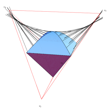
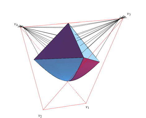
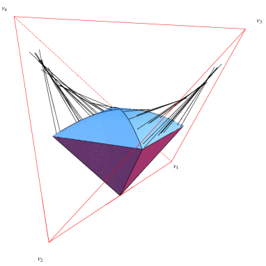
Figure 7: Fig. 7 shows that the property (ii) is not maintained for the arbitrary two-qubit states. Four figures in Fig. 7 correspond to $r=s=0.3$ (Fig. 7a), $r=-s=0.3$ (Fig. 7b), $r=s=0.5$ (Fig. 7c) and $r=-s=0.5$ (Fig. 7d). For convenience, we plot ${\cal T}$ and ${\cal L}_{r,s}$ together in each figure. Each line in Fig. 7 represents a set of ${\bm{t}}$, whose CSS has same ${\bm{\tau}}$. As Fig. 7 has exhibited, not all lines pass one of the vertices of ${\cal T}$. This fact indicates that the nice property (ii) is not maintained for the general mixtures.

In addition, one can show that the second property is not maintained too for the general mixtures. Using Eq.(6) we plot the ${\bm{\tau}}$ (correlation vector of CSS)-dependence of ${\bm{t}}$ (correlation vector of the entangled state) with varying the parameter $x$ when $\min(\mu_{-}^{\Gamma},\nu_{-}^{\Gamma})=\nu_{-}^{\Gamma}=0$. Since similar behavior arises when $\min(\mu_{-}^{\Gamma},\nu_{-}^{\Gamma})=\mu_{-}^{\Gamma}=0$, we have not included this case in Fig. 7. Four figures in Fig. 7 correspond to, respectively, $r=s=0.3$ (Fig. 7a), $r=-s=0.3$ (Fig. 7b), $r=s=0.5$ (Fig. 7c) and $r=-s=0.5$ (Fig. 7d). For convenience, we plot ${\cal T}$ and ${\cal L}_{r,s}$ together in each figure. Each line in Fig. 7 represents a set of ${\bm{t}}$, whose CSS has same ${\bm{\tau}}$. As Fig. 7 exhibits, not all lines do pass one of the vertices of ${\cal T}$. This fact indicates that unfortunately the nice property (ii) is not maintained for the arbitrary states.

The non-maintenance of the property (ii) can be proved on the analytical ground by making use of the simpler model. Let us consider $\sigma_{Z}$ in Eq.(48) and $\rho_{Z}(x)$ in Eq.(53). Then, the Bloch vectors ${\bm{r}}$, ${\bm{s}}$ and the correlation vector ${\bm{t}}$ of $\rho_{Z}(x)$ are ${\bm{r}}=(0,0,r)$, ${\bm{s}}=(0,0,s)$ and ${\bm{t}}=(t_{1},t_{2},t_{3})$, where

$$r=(R_{1}+R_{2}-R_{3}-R_{4})-x(\bar{R}_{2}-\bar{R}_{3})$$ (85)

$$s=(R_{1}-R_{2}+R_{3}-R_{4})+x(\bar{R}_{2}-\bar{R}_{3})$$

$$t_{1}=t_{2}=2Y-2x\bar{Y}\hskip 14.22636ptt_{3}=(R_{1}-R_{2}-R_{3}+R_{4})-4x\bar{R}_{1}.$$

Of course, if we take $x\rightarrow 0$ limit in Eq.(85), the corresponding quantities are the Bloch vectors and the correlation vector of $\sigma_{Z}$. Now, let us consider another state $\pi_{Z}$, which can be obtained from $\sigma_{Z}$ by changing $Y\rightarrow Y^{\prime}$ and $R_{i}\rightarrow R_{i}^{\prime}(i=1,\cdots,4)$. In order to ensure that $\pi_{Z}$ is CSS we require $Y^{\prime}=\sqrt{R_{1}^{\prime}R_{4}^{\prime}}$ and $R_{2}^{\prime}R_{3}^{\prime}\geq R_{1}^{\prime}R_{4}^{\prime}$. Then, the set of the entangled states $\xi_{Z}(x^{\prime})$, whose CSS are $\pi_{Z}$, can be obtained from $\rho_{Z}(x)$ by changing $Y\rightarrow Y^{\prime}$, $R_{i}\rightarrow R_{i}^{\prime}(i=1,\cdots,4)$ and $x\rightarrow x^{\prime}$. Thus, Bloch vectors ${\bm{r}^{\prime}}$, ${\bm{s}^{\prime}}$ and correlation vector ${\bm{t}^{\prime}}$ of $\xi_{Z}(x^{\prime})$ are ${\bm{r}^{\prime}}=(0,0,r^{\prime})$, ${\bm{s}^{\prime}}=(0,0,s^{\prime})$ and ${\bm{t}^{\prime}}=(t_{1}^{\prime},t_{2}^{\prime},t_{3}^{\prime})$, where

$$r^{\prime}=(R_{1}^{\prime}+R_{2}^{\prime}-R_{3}^{\prime}-R_{4}^{\prime})-x^{\prime}(\bar{R}_{2}^{\prime}-\bar{R}_{3}^{\prime})$$ (86)

$$s^{\prime}=(R_{1}^{\prime}-R_{2}^{\prime}+R_{3}^{\prime}-R_{4}^{\prime})+x^{\prime}(\bar{R}_{2}^{\prime}-\bar{R}_{3}^{\prime})$$

$$t_{1}^{\prime}=t_{2}^{\prime}=2Y^{\prime}-2x^{\prime}\bar{Y}^{\prime}\hskip 14.22636ptt_{3}^{\prime}=(R_{1}^{\prime}-R_{2}^{\prime}-R_{3}^{\prime}+R_{4}^{\prime})-4x^{\prime}\bar{R}_{1}^{\prime}.$$

Then, it is straightforward to show that the condition ${\bm{t}}={\bm{t}^{\prime}}$ imposes

$$x=\frac{\bar{Y}^{\prime}(\tilde{r}-\tilde{r}^{\prime})-4(Y-Y^{\prime})\bar{R}_{1}^{\prime}}{4(\bar{Y}^{\prime}\bar{R}_{1}-\bar{Y}\bar{R}_{1}^{\prime})}\hskip 14.22636ptx^{\prime}=\frac{\bar{Y}(\tilde{r}-\tilde{r}^{\prime})-4(Y-Y^{\prime})\bar{R}_{1}}{4(\bar{Y}^{\prime}\bar{R}_{1}-\bar{Y}\bar{R}_{1}^{\prime})}$$ (87)

where $\tilde{r}=R_{1}-R_{2}-R_{3}+R_{4}$ and $\tilde{r}^{\prime}=R_{1}^{\prime}-R_{2}^{\prime}-R_{3}^{\prime}+R_{4}^{\prime}$. Thus, one can compute the crossing point ${\bm{t}}={\bm{t}^{\prime}}=(\mu_{1},\mu_{2},\mu_{3})$, where $\mu_{i}$ becomes

$$\mu_{1}=\mu_{2}=\frac{4(Y\bar{Y}^{\prime}\bar{R}_{1}-Y^{\prime}\bar{Y}\bar{R}_{1}^{\prime})-\bar{Y}\bar{Y}^{\prime}(\tilde{r}-\tilde{r}^{\prime})}{2(\bar{Y}^{\prime}\bar{R}_{1}-\bar{Y}\bar{R}_{1}^{\prime})}$$ (88)

$$\mu_{3}=\frac{4(Y-Y^{\prime})\bar{R}_{1}\bar{R}_{1}^{\prime}-(\tilde{r}\bar{Y}\bar{R}_{1}^{\prime}-\tilde{r}^{\prime}\bar{Y}^{\prime}\bar{R}_{1})}{\bar{Y}^{\prime}\bar{R}_{1}-\bar{Y}\bar{R}_{1}^{\prime}}.$$

As a special case we consider the Bell-diagonal case by letting $R_{1}=R_{4}=Y=2\bar{R}_{1}=2\bar{R}_{4}=-2\bar{R}_{2}=-2\bar{R}_{3}=a$, $R_{2}=R_{3}=-2\bar{Y}=b$, $R_{1}^{\prime}=R_{4}^{\prime}=Y^{\prime}=2\bar{R}_{1}^{\prime}=2\bar{R}_{4}^{\prime}=-2\bar{R}_{2}^{\prime}=-2\bar{R}_{3}^{\prime}=a^{\prime}$ and $R_{2}^{\prime}=R_{3}^{\prime}=-2\bar{Y}^{\prime}=b^{\prime}$. Of course, one can show directly that $\rho_{Z}(x)$ and $\xi_{Z}(x^{\prime})$ are really Bell-diagonal states. Using the normalization conditions $2(a+b)=2(a^{\prime}+b^{\prime})=1$, it is easy to verify that the crossing point $(\mu_{1},\mu_{2},\mu_{3})$ is simply $\mu_{1}=\mu_{2}=1$ and $\mu_{3}=-1$, which is one of the vertices of ${\cal T}$. It is worthwhile noting that the crossing point is independent of particular choice of Bell-diagonal states $\rho_{Z}(x)$ and $\xi_{Z}(x^{\prime})$. This fact implies that all straight lines, which connect ${\bm{\tau}}$ and ${\bm{t}}$, pass one of the vertices of ${\cal T}$, which is consistent with theorem 2.

However for the arbitrary mixtures Eq.(88) implies that the crossing point $(\mu_{1},\mu_{2},\mu_{3})$ is dependent on the choice of the entangled states $\rho_{Z}(x)$ and $\xi_{Z}(x^{\prime})$. This is why the nice property (ii), which holds for the Bell-diagonal, generalized VP, and generalized Horodecki states, does not hold for the arbitrary mixture as Fig. 7 has indicated. In order to, therefore, derive the closed formula of $E_{R}(\rho)$ for the arbitrary two-qubit mixtures $\rho$, we have to understand how the property (ii) is modified when ${\bm{r}}$, ${\bm{s}}$ and ${\bm{t}}$ are arbitrary. Unfortunately, still this is an unsolved problem too.

VII Conclusion

In this paper we have considered how to find the CSS in the two-qubit system from the geometrical point of view. Of course, one can straightforwardly compute the REE of the state $\rho$ if its CSS is found. Therefore, it is important to develop a technique for finding CSS to overcome the calculational difficulty of the REE. Since, furthermore, the REE is a tight upper bound of the distillable entanglement, finding CSS is also important to understand the nature of the optimal (or near-optimal) purification protocols.

If $\rho$ is one of Bell-diagonal, generalized VP, and generalized Horodecki states, we have shown how to find the CSS of $\rho$, say $\sigma$, systematically by proving the following nice two properties: (i) The Bloch vectors of $\sigma$ are identical with those of $\rho$. (ii) The correlation vector of $\sigma$ exactly corresponds to the crossing point between the line $\ell$ and the geometrical object ${\cal L}_{r,s}$. Using these two properties it is straightforward to find the CSS of $\rho$.

As we have shown in the previous section, however, these two nice properties are not maintained for the general two-qubit states. Therefore, in order to derive the closed formula of $E_{R}(\rho)$ for the arbitrary mixture $\rho$ we have to understand how these two properties are modified when Bloch and correlation vectors of $\rho$ are arbitrary. The research into these issues is in progress and will be reported elsewhere.

Another interesting issue, which we will go further, is to explore the REE and the distillable entanglement for the higher-qubit or qudit systems. Few years ago, the analytical expressions of the distillable entanglement are obtained for some higher-dimensional bipartite statesghosh01 ; chen02 ; chen03 . Authors in those references used the upper-bound criterion $D\leq E_{R}$ and separability property of the Smolin’s unlockable statesmolin00 in various cuts. We would like to modify Eq.(6) to be applicable not only for low-rank $\sigma^{*}$ but also for higher-dimensional system. If the generalization of Eq.(6) is possible, we can use it to compute the REE and the distillable entanglement for many more higher-dimensional states. It may enable us to understand the nature of the optimal (or near-optimal) purification protocols. This work is in progress too.

References

(1) C. H. Bennett, G. Brassard, C. Crépeau, R. Jozsa,
A. Peres and W. K. Wootters, Teleporting an Unknown Quantum State via
Dual Classical and Einstein-Podolsky-Rosen Channles,
Phys. Rev. Lett. 70 (1993) 1895.
(2) C. H. Bennett and S. J. Wiesner, Communication via one-
and two-particle operators on Einstein-Podolsky-Rosen states, Phys. Rev. Lett.
69 (1992) 2881.
(3) V. Scarani, S. Lblisdir, N. Gisin and A. Acin, Quantum cloning,
Rev. Mod. Phys. 77 (2005) 1225 [quant-ph/0511088] and references therein.
(4) A. K. Ekert,
Quantum Cryptography Based on Bell’s Theorem, Phys. Rev. Lett.
67 (1991) 661.
(5) G. Vidal, Efficient classical simulation of slightly
entangled quantum computations, Phys. Rev. Lett. 91 (2003)
147902 [quant-ph/0301063].
(6) M. A. Nielsen and I. L. Chuang, Quantum Computation and
Quantum Information (Cambridge University Press, Cambridge, England, 2000).
(7) Y. Shimoni, D. Shapira and O. Biham, Characterization of pure quantum states of multiple qubits,
Phys. Rev. A69 (2004) 062303 [quant-ph/0309062].
(8) B. P. Lanyon, M. Barbieri, M. P. Almeida and A. G. White, Experimental quantum computing without entanglement,
Phys. Rev. Lett. 101 (2008) 200501 [arXiv:0807.0668 (quant-ph)].
(9) E. Biham, G. Brassard, D. Kenigsberg and T. Mor, Quantum computing without entanglement,
Theor. Comp. Sci. 320 (2004) 15 [quant-ph/0306182].
(10) C. H. Bennett, D. P. DiVincenzo, J. A. Smolin and W. K. Wootters,
Mixed-state entanglement and quantum error correction, Phys. Rev. A54
(1996) 3824 [quant-ph/9604024].
(11) V. Vedral, M. B. Plenio, M. A. Rippin and P. L. Knight, Quantifying
Entanglement, Phys. Rev. Lett. 78 (1997) 2275 [quant-ph/9702027].
(12) V. Vedral and M. B. Plenio, Entanglement measures and purification procedures,
Phys. Rev. A57 (1998) 1619 [quant-ph/9707035].
(13) E. M. Rains, Rigorous treatment of distillable entanglement, Phys. Rev. A60
(1999) 173 [quant-ph/9809078].
(14) E. M. Rains, Bound on distillable entanglement, Phys. Rev. A60 (1999) 179 [quant-ph/9809082].
(15) J. A. Smolin, Four-party unlockable bound entangled state, Phys. Rev. A63 (2001)
032306 [quant-ph/0001001].
(16) S. Ghosh, G. Kar, A. Roy, A. Sen and U. Sen, Distinguishability of Bell States, Phys. Rev. Lett.
87 (2001) 277902 [quant-ph/0106148].
(17) Y. X. Chen, J. S. Jin and D. Yang, Distillation of multiple copies of Bell states, Phys. Rev.
A67 (2003) 014302 [quant-ph/0204004].
(18) D. Yang and Y. X. Chen, Mixture of multiple copies of maximally entangled states is quasipure,
Phys. Rev. A69 (2004) 024302 [quant-ph/0304194].
(19) R. Horodecki, P. Horodecki, M. Horodecki, and K. Horodecki, Quantum Entanglement,
Rev. Mod. Phys. 81 (2009) 865 [quant-ph/0702225] and references therein.
(20) M. Hayashi, D. Markham, M. Murao, M. Owari and S. Virmani,
Bounds on Multipartite Entangled Orthogonal State Discrimination Using Local Operations and Classical
Communication, Phys. Rev. Lett. 96 (2006) 040501 [quant-ph/0506170].
(21) T. C. Wei, Relative entropy of entanglement for multipartite mixed states:
Permutation-invariant states and Dür states, Phys. Rev. A78 (2008) 012327 [arXiv:0805.1090 (quant-ph)].
(22) A. Miranowicz and S. Ishizaka, Closed formula for the relative entropy of entanglement,
Phys. Rev. A78 (2008) 032310 [arXiv:0805.3134 (quant-ph)].
(23)W. K. Wootters, Entanglement of Formation of an Arbitrary State of
Two Qubits, Phys. Rev. Lett. 80, 2245 (1998) [quant-ph/9709029].
(24) O. Krueger and R. F. Werner, Some Open Problems in Quantum Information Theory, quant-ph/0504166.
(25) R. Horodecki and M. Horodecki, Information-theoretic aspects of inseparability of mixed states, Phys. Rev.
A54 (1996) 1838 [quant-ph/9607007].
(26) E. Jung, M. R. Hwang, D. K. Park, L. Tamaryan and S. Tamaryan, Three-Qubit Groverian Measure,
Quant. Inf. Comp. 8 (2008) 0925 [arXiv:0803.3311 (quant-ph)].