A theory of MHD instability of an inhomogeneous plasma jet

Abstract

A problem of the instability of an inhomogeneous axisymmetric plasma jet in a parallel magnetic field is solved. The jet boundary becomes, under certain conditions, unstable relative to magnetosonic oscillations (Kelvin-Helmholtz instability) in the presence of a shear flow at the jet boundary. Because of its internal inhomogeneity the plasma jet has resonance surfaces, where conversion takes place between various modes of plasma MHD oscillations. Propagating in inhomogeneous plasma, fast magnetosonic waves drive the Alfven and slow magnetosonic oscillations, tightly localized across the magnetic shells, on the resonance surfaces. MHD oscillation energy is absorbed in the neighbourhood of these resonance surfaces. The resonance surfaces disappear for the eigen-modes of slow magnetosonic waves propagating in the jet waveguide. The stability of the plasma MHD flow is determined by competition between the mechanisms of shear flow instability on the boundary and wave energy dissipation because of resonant MHD-mode coupling. The problem is solved analytically, in the WKB approximation, for the plasma jet with a boundary in the form of a tangential discontinuity over the radial coordinate. The Kelvin-Helmholtz instability develops if plasma flow velocity in the jet exceeds the maximum Alfven speed at the boundary. The stability of the plasma jet with a smooth boundary layer is investigated numerically for the basic modes of MHD oscillations, to which the WKB approximation is inapplicable. A new ”global” unstable mode of MHD oscillations has been discovered which, unlike the Kelvin-Helmholtz instability, exists for any, however weak, plasma flow velocities.

1 Introduction

Shear plasma flows in magnetic field are encountered in many problems in magnetohydrodynamics. Of most interest are usually unstable oscillations developing in a shift layer. Thus, many kinds of geomagnetic field oscillations related to the Kelvin-Helmholtz instability develop on the Earth’s magnetospheric boundary when the solar wind plasma flows around it [1, 2]. Similar instabilities arise in differentially rotating plasma shells of stars [3]. The problem of the instability of the plasma configuration boundary in experimental installations where the plasma was confined magnetically has been discussed widely enough [4, 5]. In such installations, plasma injected along the magnetic field lines becomes unstable [6].

Analytical studies devoted to shear flow stability are often stated for two-layer medium models where fluid, gas or plasma move in two homogeneous half-spaces separated by a flat shift layer of velocity [1, 7]. Using such models enables one to progress far enough in constructing analytical solutions to hydrodynamic (or magnetohydrodynamic) equations describing unstable oscillation modes. However, real shear flows occur, as a rule, in an inhomogeneous medium in a layer of finite thickness. Constructing analytical solutions in such models is only possible for several extreme cases [8]. Solutions to corresponding equations are often obtained by numerical integration [9]. As a rule, all effects related to medium inhomogeneity are ascribed, in these models, to the shift layer, while the medium away from it is supposed to be homogeneous. The solutions obtained in this way have a rather strong limitation regarding their applicability area as well.

In many real events the medium remains inhomogeneous (though the scale of the inhomogeneity is smaller than in the shift layer) even far from the shift layer. This inhomogeneity can also play a considerable role in forming the conditions under which the unstable oscillation modes develop in the shift layer [10]. For example, in the inhomogeneous layer, the resonance surfaces can exist where there is a coupling of various modes of MHD oscillations. When fast magnetosonic (FMS) waves propagate in inhomogeneous plasma they can drive the Alfven and slow magnetosonic (SMS) oscillations tightly localized across magnetic shells, on the resonance surfaces [11]. This results in the oscillation energy absorbed by particles of the background plasma, heating up in the process [12, 13]. The mechanism stabilizes the unstable modes.

Shear flows bounded in space also have their specific features. Such jet flows arise, for example, when plasma clusters are injected into magnetic traps along the magnetic field lines [14]. The same conditions arise when plasma filaments erupt from the Sun surface in the corona [15], and also when the solar wind plasma flows round a planet’s magnetosphere [1, 16]. The model of a cylindrical plasma jet propagating parallel to the magnetic field lines is obviously closest to reality in all these situations. There are a few studies devoted to the stability of hydrodynamic and magnetohydrodynamic flows in cylindrical models (see [16, 17]).

This work tackles the problem of stability of a cylindrical plasma jet in a parallel magnetic field. The plasma in the jet is assumed to be homogeneous over the azimuth and inhomogeneous over the radius. The velocity of plasma in the jet is supposed to be homogeneous. The shear flow occurs in a layer of finite thickness at the plasma jet boundary. For a qualitative understanding of the structure and dynamics of the unstable oscillation modes, this problem is solved in the WKB approximation over the radial coordinate. The boundary of the plasma jet is assumed to be in the form of a tangential discontinuity. The solution to the problem when the boundary has the form of a smooth transition layer is obtained numerically for the first harmonics of unstable oscillations, for which the WKB approximation is inapplicable.

This paper is structured as follow. The model of the medium is presented and the basic equations of the problem under study are derived in Section 2. Section 3 is a qualitative examination of the structure of the radial component of the wave vector in the WKB approximation, as well as deriving the boundary conditions and the matching condition on the jet boundary for unstable MHD oscillations in question. Section 4 examines the structure of the forced modes and eigen-modes of MHD oscillations of the plasma jet in the WKB approximation. The dependence on the plasma flow velocities of the increment of unstable oscillations of the plasma jet (with a boundary in the form a tangential discontinuity) is analytically studied in Section 5. Section 6 provides a numerical solution to the same problem for a plasma jet with its boundary in the form of a smooth transition layer. Section 7 explores the instability of the ”global modes” of plasma jet oscillations. The Conclusion lists the main results of this work.

2 Model medium and basic equations

Let us consider a model cylindrical plasma jet presented in fig.1-2. Let us introduce a cylindrical coordinates system ($r,\phi,z$) where the origin $r=0$ coincides with the jet axis. We assume the background magnetic field to be directed along the $z$ axis and be homogeneous (but not identical) inside and outside the plasma jet. In calculations for the jet boundary in the tangential discontinuity approximation, the parameters of the medium on its conventional boundary $r=r_{b}$ will have a subscript _I - inside, and _II outside. We will consider the plasma in the jet to be moving along the $z$ axis at velocity $v_{0}$, and the plasma outside of the jet to be immobile (see fig.1). Transition from the jet parameters to the parameters outside occurs within a narrow transition layer of thickness $\Delta_{r}\ll r_{b}$. The plasma density distribution over the radius will be considered as maximum at the jet axis and decreasing to a minimum toward the boundary. We assume the magnetic field inside the jet to be greater than outside. The distribution of the Alfven speed $A=B_{0}/\sqrt{4\pi\rho_{0}}$ over the radius has the form presented qualitatively in fig.1-2. Such a distribution of plasma parameters occurs in magnetic arches on the Sun, in the magnetotail of the Earth’s magnetosphere, as well as in laboratory installations with magnetic plasma confinement of the theta-pinch type.

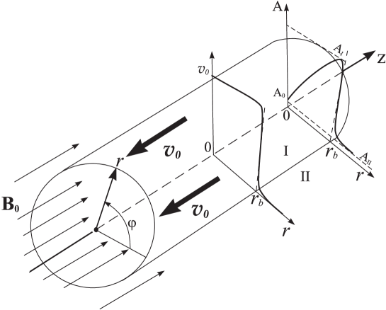
Figure 1: A model of cylindrical plasma jet whose plasma motion is directed against the background magnetic field $\bi{B_{0}}$. The distributions of the velocity profile of moving plasma ${v_{0}}(r)$ and of the Alfven speed $A(r)$ are presented schematically.

To describe such a plasma configuration we used a set of ideal MHD equations of the form

$$\rho\frac{d\bar{\bi{v}}}{dt} = -\-\nabla\bar{P}+\frac{1}{4\pi}[\mathop{\mathrm{curl}}\bar{\bi{B}}\times\bar{\bi{B}}],$$ (1a)

$$\frac{\partial\bar{\bi{B}}}{\partial{}t} = \mathop{\mathrm{curl}}[\bar{\bi{v}}\times\bar{\bi{B}}],$$ (1b)

$$\frac{\partial\bar{\rho}}{\partial{}t} + \nabla(\rho\bar{\bi{v}})=0,$$ (1c)

$$\frac{d}{dt}\frac{\bar{P}}{\bar{\rho}^{\gamma}} = 0,$$ (1d)

where $\bar{\bi{B}},\ \bar{\bi{v}}$ are vectors of the magnetic field and velocity of the plasma motion, $\bar{\rho},\ \bar{P}$ are the plasma density and pressure, $\gamma=5/3$ is the adiabatic index. Let us assume the wave-related disturbance to be weak enough, allowing for the initial set of equations to be linearized. Let us denote the parameters of the unperturbed plasma with a subscript of zero, while leaving the wave-related parameters unindexed: $\bar{\bi{B}}=\bi{B_{0}}+\bi{B},\ \bar{\bi{v}}=\bi{v_{0}}+\bi{v},\ \bar{\rho}=\rho_{0}+\rho,\bar{P}=P_{0}+P$. In the zero approximation the $r$ component of equation (1a) in steady state ($\partial/\partial t=0$) yields the equilibrium condition for a plasma configuration

$$P_{0}+\frac{B_{0}^{2}}{8\pi}=const,$$ (1b)

which determines an equilibrium distribution of the plasma pressure $P_{0}(r)$ for a fixed distribution of $B_{0}(r)$. This pressure determines the distribution of the sound velocity in plasma $S=\sqrt{\gamma P_{0}/\rho_{0}}$ and a corresponding distribution of SMS-wave velocity $C_{s}=AS/\sqrt{A^{2}+S^{2}}$ in fig. 2. Let us assume the magnetic field to be almost constant inside and outside the plasma jet, changing only in a thin transition layer of thickness $\Delta_{r}\ll r_{b}$. Then it follows from the equilibrium condition (1b) that the plasma pressure also varies inside the transition layer only. We denote the component of the vector of the disturbed plasma velocity in a wave in the $r$ axis direction $v_{r}=\mathrm{d}\zeta/\mathrm{d}t\equiv\partial\zeta/\partial t+(\mathbf{\bi{v}_{0}\nabla})\zeta$, where $\zeta$ is the displacement of a plasma element. Let us consider the harmonic of a wave in the form $\exp(ik_{z}z+im\phi-i\omega t)$, where $k_{z}$ is the component of the wave vector in the $z$ axis direction, $m=0,1,2,3...$ is azimuthal wave number, $\omega$ is wave frequency. Linearizing the set of equations (1a)-(1d) and expressing the other components of the oscillation field through $\zeta$, we obtain:

$$v_{r}=-i\bar{\omega}\zeta,\ \ \ \ \ v_{\phi}=-\frac{1}{K_{s}^{2}}\left(A^{2}+\frac{K_{A}^{2}S^{2}}{\chi_{S}^{2}}\right)\frac{m}{\bar{\omega}r^{2}}\frac{\partial r\zeta}{\partial r},$$ (1ca)

$$v_{z}=-\frac{k_{z}K_{A}^{2}S^{2}}{\bar{\omega}\chi_{S}^{2}r}\frac{\partial r\zeta}{\partial r}-v_{0}^{\prime}\zeta,$$

$$B_{r}=-ik_{z}B_{0}\zeta,\ \ \ \ B_{\phi}=-\frac{k_{z}B_{0}}{\bar{\omega}}v_{\phi},\ \ \ B_{z}=-\frac{K_{A}^{2}B_{0}}{\chi_{S}^{2}}\left(1-\frac{k_{z}^{2}S^{2}}{\bar{\omega}^{2}}\right)\frac{1}{r}\frac{\partial r\zeta}{\partial r}-B_{0}^{\prime}\zeta,$$

$$P=-\gamma P_{0}\frac{K_{A}^{2}}{\chi_{S}^{2}}\frac{1}{r}\frac{\partial r\zeta}{\partial r}+\left(\frac{B_{0}^{2}}{8\pi}\right)^{\prime}\zeta,$$ (1cb)

where

$$K_{A}^{2}=1-\frac{k_{z}^{2}A^{2}}{\bar{\omega}^{2}},\ \ \ \ \ \ \ K_{s}^{2}=K_{A}^{2}-\frac{m^{2}A^{2}}{r^{2}\bar{\omega}^{2}},$$

$$\chi_{S}^{2}=1-\frac{m^{2}/r^{2}+k_{z}^{2}}{\bar{\omega}^{2}}\left(A^{2}+S^{2}-\frac{k_{z}^{2}A^{2}S^{2}}{\bar{\omega}^{2}}\right),$$

$\bar{\omega}=\omega-k_{z}v_{0}$ is an oscillation frequency modified by Doppler’s effect. For the displacement $\zeta$ we obtain the equation

$$\frac{\partial}{\partial r}\,\,\frac{\rho_{0}\Omega^{2}}{k_{r}^{2}}\,\,\frac{1}{r}\frac{\partial r\zeta}{\partial r}+\rho_{0}\Omega^{2}\zeta=0,$$ (1cd)

where $\Omega^{2}=\omega^{2}-k_{z}^{2}A^{2}$,

$$k_{r}^{2}=\frac{\bar{\omega}^{4}}{\bar{\omega}^{2}(A^{2}+S^{2})-k_{z}^{2}A^{2}S^{2}}-k_{z}^{2}-\frac{m^{2}}{r^{2}}=$$ (1ce)

$$k_{z}^{2}\left(\frac{\bar{\omega}_{A}^{4}/(1+\beta^{*})}{(\bar{\omega}_{A}^{2}-\bar{\omega}_{S}^{2})}-1-\frac{m^{2}}{k_{z}^{2}r^{2}}\right)=$$

$$\frac{k_{z}^{2}}{1+\beta^{*}}\frac{(\bar{\omega}_{A}^{2}-\bar{\omega}_{A1}^{2})(\bar{\omega}_{A}^{2}-\bar{\omega}_{A2}^{2})}{(\bar{\omega}_{A}^{2}-\bar{\omega}_{s}^{2})},$$

and the notations are $\bar{\omega}_{A}=\bar{\omega}/k_{z}A(r)$, $\bar{\omega}_{S}=\sqrt{\beta^{*}/(1+\beta^{*})}$, $\beta^{*}=S^{2}/A^{2}$, whereas $\bar{\omega}_{A1}^{2},\bar{\omega}_{A2}^{2}$ are the roots of a biquadratic (with respect to $\bar{\omega}_{A}$) equation $k_{r}^{2}=0$.

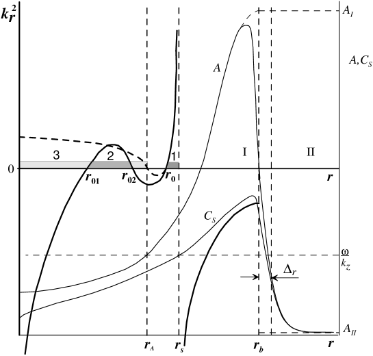
Figure 2: Distribution of the Alfven speed $A(r)$ and velocities of the SMS waves $C_{s}(r)$ inside and outside of the plasma jet (the thin lines and right-hand vertical axis). Distribution of the squared WKB component of the wave vector $k^{2}_{r}(r)$ in the plasma jet (the thick lines; for the mode $m=0$ dashed line, left vertical axis). The $r_{A}$ and $r_{S}$ coordinates correspond to the resonance surfaces for the Alfven and SMS-oscillations in the jet, respectively; $r_{0},r_{01},r_{02}$ are the turning points. The numerals and shades of gray demonstrate the transparency regions: (1) for SMS waves, (2) for FMS waves ($m\neq 0$), and (3) $m=0$.

Note that the expression $\beta^{*}$ coincides, within a factor close to unity, with the well known parameter $\beta=8\pi P_{0}/B_{0}^{2}$ - the gas-kinetic plasma to magnetic pressure ratio. It can be seen from (1cd) that $k_{r}^{2}$ is the square of the $r$-component of the wave vector in the WKB approximation when the solution to (1cd) may be presented in the form $\zeta\sim\exp(i\int k_{r}dr)$.

3 The distribution of $k_{r}^{2}(r)$, the matching conditions on the plasma jet boundary and boundary conditions

Solving the problem in the WKB approximations is determined by the magnitude of the wave vector component $k_{r}^{2}(r)$ on both sides of the plasma jet boundary presented in the form of a tangential discontinuity. We will analyse the behaviour of $k_{r}^{2}(r)$ inside and outside the jet. For convenience, our subsequent calculations will involve the frame of reference moving with the flux plasma at velocity $\bi{v}_{0}$. In this frame of reference plasma is immobile in the plasma flux rope, while moving at velocity $-v_{0}$ outside of it. The distribution of $k_{r}^{2}(r)$ in the plasma flux rope is presented qualitatively in fig. 2. This figure presents the distribution of $k_{r}^{2}(r)$ for such values of $m,k_{z}$ and $\omega$ for which all possible resonance surfaces and turning points are present in the plasma flux rope.

The turning points are determined by zeros of the function $k_{r}^{2}(r)$. In the distribution in fig. 2 their number can vary from one ($r_{0}$) to three ($r_{0},r_{01},r_{02}$). The number of turning points is determined by the parameters $m,k_{z}$ and $\omega$. Thus, for the axisymmetric mode $m=0$, the turning point $r_{02}$ is absent, whereas another one - $r_{01}$ coincides with the point $r_{A}$, that determines the location of the resonance surface for Alfven wave when $m\neq 0$. A transparency region (where $k_{r}^{2}(r)>0$) can exist for the FMS waves in the plasma flux rope - this region is located in the range $r_{01}\leq r\leq r_{02}$ when $m\neq 0$, and in the range $0\leq r\leq r_{A}$ when $m=0$. The transparency region for SMS waves is located in the interval $r_{0}\leq r\leq r_{s}$ (where $r_{s}$ is a resonance surface for the SMS oscillations).

Resonance surfaces are determined by the singular points of equation (1cd) where the coefficient of the higher derivative reduces to zero. One of them – the Alfven resonance point $r_{A}$ determined by the equation $\Omega^{2}(r_{A})=0$ – is located in the opacity region in the interval $(r_{02},r_{0})$. When $m=0$ the point $r_{A}$ is the turning point and is not singular (the coefficient of the higher derivative here does not reduce to zero). The second singular point – magnetosonic resonance point $r_{s}$ – is determined by the denominator in the expression (1ce) becoming zero, yielding a local dispersion equation for SMS waves when $|k_{r}^{2}|\rightarrow\infty$: $\omega^{2}=k_{z}^{2}C_{s}^{2}(r_{s})$. The point $r_{s}$ is located farther along the radius than the turning point $r_{0}$, and the transparency region for the SMS waves is located between them. The opacity region is in the range $r_{s}<r<r_{b}$.

It is evident from (1ce) that the behaviour of $k_{r}^{2}(r)$ in the range $0<r<r_{b}$ depends on the magnitude of $\bar{\omega}_{A}(r)$ at the ends of the interval. It is possible to see the distribution of $k_{r}^{2}(r)$ mentally moving the function $k_{r}^{2}(r)$ shown in fig.2 from left to right. When $\omega^{2}_{0}<\omega_{SI}^{2}$ (where $\omega^{2}_{0}\equiv\bar{\omega}_{A}^{2}(0)$, $\omega_{SI}^{2}=const$ is the magnitude of $\bar{\omega}_{S}^{2}$ in a plasma flux rope) we have $k_{r}^{2}(r)<0$ over the entire cross-section of the jet, i.e. the entire jet is an opacity region. It is possible to regard the entire interval $0<r<r_{b}$ as the part of the $k_{r}^{2}(r)$ plot, presented in fig.2, corresponding to the opacity region $r_{s}<r<r_{b}$. The point of magnetosonic resonance $r_{s}$ is absent from the system – the rest of the plot in fig. 2 can be imagined on the left of the point $r=0$. When $\omega^{2}_{0}$ increases (due to growing parallel phase velocity $\omega/k_{z}$) this plot moves from left to right in the range $0<r<r_{b}$. The resonance surface for SMS waves $r_{s}$ (for $\omega_{SI}^{2}<\omega^{2}_{0}$), the turning point for SMS waves $r_{0}$ (for the case $m\neq 0$, the points $r_{s}$ and $r_{0}$ appear only together), the resonance surface for Alfven waves $r_{A}$, and turning points $r_{01}$ and $r_{02}$ (for $m\neq 0$) appear sequentially in the system.

Similarly, for $\omega_{SI}^{2}<\omega^{2}_{b}$ (where $\omega^{2}_{b}\equiv\bar{\omega}_{A}^{2}(r_{b})$) the resonance surface for SMS waves disappears ($r_{s}$ is virtually displaced to the right of $r_{b}$) from the system. When $\omega^{2}_{b}$ then increases, the points $r_{0}$, $r_{A}$ (for $m=0$ the entire jet becomes a transparency region) and $r_{01}$ disappear sequentially. The point $r_{02}\rightarrow 0$ when $\omega^{2}_{b}\rightarrow\infty$. This may be imagined by shifting the function $k_{r}^{2}(r)$ plot, presented in fig.2, farther to the right through the point $r=r_{b}$. Thus, depending on the magnitude of $\omega/k_{z}$, both the transparency region and the opacity region for the waves in question can adjoin the boundary inside the jet.

To picture the behaviour of $k_{r}^{2}(r)$ outside the jet, we will consider the functions $\bar{\omega}_{A1}^{2}(r),\bar{\omega}_{A2}^{2}(r)$, presented in fig.3. As follows from the last expression of (1ce), when $\bar{\omega}_{AII}^{2}<\bar{\omega}_{SII}^{2}$ (where $\bar{\omega}_{AII}^{2}\equiv\bar{\omega}_{A}^{2}(r\rightarrow\infty)$, $\bar{\omega}_{SII}^{2}\equiv\bar{\omega}_{S}^{2}(r\rightarrow\infty)$) - the outside jet region adjoining the boundary $r=r_{b}$ is an opacity region for the waves in question. When $\bar{\omega}_{SII}^{2}<\bar{\omega}_{AII}^{2}<\bar{\omega}_{A2b}^{2}$ - the outside region is transparent, and for $\bar{\omega}_{A2b}^{2}<\bar{\omega}_{AII}^{2}<\beta^{*}_{II}$ the transparency region shifts to $r>r_{1}>r_{b}$. In the interval $\beta^{*}_{II}<\bar{\omega}_{AII}^{2}<1+\beta^{*}_{II}$ the outside region adjoining the boundary is opaque, but is transparent when $\bar{\omega}_{A1b}^{2}<\bar{\omega}_{AII}^{2}$.

Figure 3: Distribution of the functions $\bar{\omega}_{A1}^{2}(r),\bar{\omega}_{A2}^{2}(r)$ and transparency regions (shown in grey) for SMS (1) and FMS waves (2,3,4), when $r>r_{b}$. Two possible magnitudes of $\bar{\omega}_{AII}^{2}\equiv\bar{\omega}_{A}^{2}(r\rightarrow\infty)$ (horizontal bold dashed lines) are presented, for which the turning points $r_{1,2}$ exist in the regions outside of the jet.

Thus, depending on the magnitude of $\bar{\omega}_{AII}^{2}$ determined by the wave phase velocity given the Doppler displacement of frequency for the oscillations under study $\bar{\omega}/k_{z}$, the boundary can also adjoin both the transparency and the opacity region outside the jet. As was shown above, the transparency or opacity of the region adjoining the boundary inside the jet is determined by the magnitude of the parallel phase velocity $\omega/k_{z}$. The solutions describing the oscillations in the transparency and the opacity regions adjoining the boundary outside and inside the jet can be combined in all possible combinations in the matching condition.

It is easy to obtain the matching condition for the solutions on the plasma jet boundary by integrating the equation (1cd) in a narrow interval ($r_{b}-\varepsilon,r_{b}+\varepsilon$):

$$\left.\frac{\rho_{0}\Omega^{2}}{k_{r}^{2}}\frac{\partial\ln\zeta}{\partial r}\right|_{r_{b}-\varepsilon}=\left.\frac{\rho_{0}\Omega^{2}}{k_{r}^{2}}\frac{\partial\ln\zeta}{\partial r}\right|_{r_{b}+\varepsilon},$$ (1cf)

where $\varepsilon\rightarrow 0$. Using the expressions (1c), (1cb) it is possible to show that (1cf) is similar to the requirements for the plasma to be identically displaced on both sides of the boundary ($\zeta_{r_{b}-\varepsilon}=\zeta_{r_{b}+\varepsilon}$ is the condition of impermeability) and for the total perturbed pressure to be sustained across the boundary ($(P+B_{z}B_{0}/4\pi)_{r_{b}-\varepsilon}=(P+B_{z}B_{0}/4\pi)_{r_{b}+\varepsilon}$).

Now let us define the boundary conditions for the problem. When $r\rightarrow 0$ the finite magnitude of the desired solution is a natural requirement. As to the boundary condition for $r\rightarrow\infty$ its determination is related to the causality principle. In this problem, we will be interested in solutions to (1cd) describing unstable modes of the plasma jet oscillations. For such solutions, oscillations far from the shift layer are running away from the shear flow that generated them, according to the causality principle. In other words, the energy flux of these waves should be directed out of the shift layer.

It should be noted when dealing with unstable oscillations that the wave vector component $k_{r}$ in the asymptotics is complex. For any weak unstable oscillations, it is formally possible to introduce the concept of waves running from the shift layer, for which ${\rm Re}(v_{gr})>0$ when $r\rightarrow\infty$, where $v_{gr}=\partial\omega/\partial k_{r}$ is the group velocity with which the wave energy is transferred over the radius $r$. The energy conservation law

$$\frac{\partial\mathcal{E}}{\partial t}+\frac{1}{r}\frac{\partial}{\partial r}(r\mathbf{v}_{gr}\mathcal{E})=0,$$

where $\mathcal{E}$ is wave energy density, quadratic on the oscillation amplitude, implies that ${\rm Im}(k_{r})>0$ when $r\rightarrow\infty$ for monochromatic unstable oscillations ($\rm{Im}(\omega)>0$). This results in an exponentially decreasing amplitude of oscillations escaping from the shift layer. A specific expression for the group velocity when $r\rightarrow\infty$ can be obtained by differentiating the expression (1ce) with respect to $\omega$:

$$v_{gr}=A_{II}\frac{1+\beta^{*}_{II}}{k_{z}}{\rm Re}k_{rII}\frac{\left[\bar{\omega}_{A}^{2}-\bar{\omega}_{SII}^{2}\right]^{2}}{\bar{\omega}_{A}^{3}\left[\bar{\omega}_{A}^{2}-2\bar{\omega}_{SII}^{2}\right]}.$$ (1cg)

The boundary condition for the wave running from the shift layer when $r\rightarrow\infty$ has the form

$$\frac{\partial\zeta}{\partial r}=ik_{rII}\zeta,$$ (1ch)

and the sign of $k_{rII}=\pm\sqrt{k_{rII}^{2}}\equiv k_{r}(r\rightarrow\infty)$ is determined by the requirement ${\rm Re}(v_{gr})>0$.

4 Structure of MHD oscillations in the jet in the WKB approximation

In order to understand qualitatively the structure of the oscillations in the plasma jet, let us consider a problem for the MHD oscillations with parameters permitting us to use the WKB approximation far from the turning points and resonance surfaces. We will search for solutions in the neighbourhoods of these points by linearizing the coefficients in (1cd) and subsequently matching the solutions with the solutions obtained in the WKB approximation. To make a complete picture of the wave field structure, let us consider oscillations with parameters corresponding to the distribution of $k_{r}^{2}(r)$ in fig.2, presenting all possible singular and turning points. Let us consider the structure of the forced and eigen-oscillations of the plasma jet separately.

4.1 The structure of forced oscillations in the plasma jet

Let us consider the case of forced MHD oscillations of the plasma jet, with a source located at its boundary.

When $r\rightarrow 0$ equation (1cd) can be approximately presented in the form:

$$r^{2}\zeta^{\prime\prime}+r^{\sigma}\zeta^{\prime}+(k_{r0}^{2}r^{2}-1)\zeta=0,$$

where $k_{r0}^{2}\equiv k_{r}^{2}(r\rightarrow 0)$ (for $m\neq 0$ we have $k_{r0}^{2}\approx-m^{2}/r^{2}$), $\sigma=1$ when $m=0$ and $\sigma=3$ when $m\neq 0$. A solution which is finite when $r\rightarrow 0$ has the form:

$$\zeta=C_{1}\left\{\begin{array}[]{lcr}J_{1}(\sqrt{k_{r0}^{2}}r),&for\ m=0,\\ r^{m-1},&for\ m\neq 0,\end{array}\right.$$ (1ci)

where $C_{1}$ is an arbitrary constant, $J_{1}(\sqrt{k_{r0}^{2}}r)$ is the Bessel function ($J_{1}(\sqrt{k_{r0}^{2}}r)\stackrel{{\scriptstyle r\rightarrow 0}}{{\approx}}\sqrt{k_{r0}^{2}}r/2$). The subsequent calculations will concern the case $m\neq 0$.

Let us present the WKB solution in the opacity region $0<r<r_{01}$, matched with (1ci), in the form

$$\zeta=C_{2}\frac{(-k_{r}^{2})^{1/4}}{\sqrt{\rho_{0}\Omega^{2}r}}\exp\left(\int_{r_{01}}^{r}\sqrt{-k_{r}^{2}}dr^{\prime}\right),$$ (1cj)

where $C_{2}$ is an arbitrary constant. Matching (1ci) to (1cj) we obtain a relation for the constants $C_{1}=C_{2}\exp{(\psi_{1})}/\bar{r}^{m}\sqrt{\rho_{0}\Omega^{2}_{0}/m}$, where $\psi_{1}=\int_{r_{01}}^{\bar{r}}\sqrt{-k_{r}^{2}}dr$, and $\bar{r}>0$ is an arbitrary point in the neighbourhood of $r=0$.

Solution in the neighbourhood of the turning point $r=r_{01}$. Let us differentiate (1cd) with respect to $r$, introduce the notation $u=(1/k_{r}^{2})\partial\zeta/\partial r$ and, linearizing $k_{r}^{2}\approx\xi_{1}/a_{1}^{2}$ close to $r=r_{01}$ (where $a_{1}^{-3}=(\partial k_{r}^{2}/\partial r)_{r=r_{01}}$, $\xi_{1}=(r-r_{01})/a_{1}$), will yield an equation

$$\frac{\partial^{2}u}{\partial\xi_{1}^{2}}+\xi_{1}u=0.$$ (1ck)

Its solution matched to (1cj) has the form

$$u=C_{3}Ai(-\xi_{1}),$$ (1cl)

where $Ai(z)$ is the Airy function. Matching this solution to (1cj) yields a relation for the constants $C_{3}=2C_{2}\sqrt{\pi a_{1}/\rho_{01}\Omega^{2}_{1}r_{01}}$. Hereafter the subscripts ${}_{0},_{1},_{2},_{A},_{S}$ denote the parameters at the corresponding points $r_{0},r_{01},r_{02},r_{A},r_{S}$.

The WKB solution in the transparency region $r_{01}<r<r_{02}$, matched to (1cl) has the form

$$u=\frac{C_{4}}{\sqrt{\rho_{0}\Omega^{2}k_{r}r}}\sin\left(\int_{r_{01}}^{r}k_{r}dr^{\prime}+\frac{\pi}{4}\right),$$ (1cm)

where $C_{4}=2C_{2}$.

The solution in the neighbourhood of the turning point $r=r_{02}$ may be obtained using linearization $k_{r}^{2}\approx-\-\xi_{2}/a_{2}^{2}$ ($a_{2}^{-3}=(\partial k_{r}^{2}/\partial r)_{r=r_{02}}$, $\xi_{2}=(r-r_{02})/a_{2}$) and obtaining an equation similar to (1ck) accurate within the substitution $\xi_{1}\rightarrow-\xi_{2}$. Its solution matched to (1cm) is

$$u=C_{5}Ai(\xi_{2})+C_{6}Bi(\xi_{2}),$$ (1cn)

where $Ai(z),Bi(z)$ are the Airy functions. We have the constants $C_{5}=C_{4}\sqrt{\pi a_{2}/\rho_{02}\Omega^{2}_{2}r_{02}}\sin{\psi_{2}}$, $C_{6}=C_{4}\sqrt{\pi a_{2}/\rho_{02}\Omega^{2}_{2}r_{02}}\cos{\psi_{2}}$, where $\psi_{2}=\int_{r_{01}}^{r_{02}}k_{r}dr$. If $\psi_{2}=\pi(n+1/2)$ ($n=0,1,2...$) and $C_{6}=0$, then to the right of $r_{02}$ in the opacity region we have a solution exponentially decreasing in amplitude (the asymptotics of the functions when $z\rightarrow\infty$: $Ai(z)=\exp[-(2/3)z^{3/2}]/2\sqrt{\pi\sqrt{z}},\ \ Bi(z)=\exp[(2/3)z^{3/2}])/\sqrt{\pi\sqrt{z}}$). This condition means that the eigen-waveguide mode of FMS waves is captured in the transparency region ($r_{01},r_{02}$). As to the case $m=0$, a solution similar to (1cm) is obtained for the transparency region ($0,r_{A}$).

The WKB solution in the opacity region $r_{02}<r<r_{A}$ will be presented in the form:

$$\zeta=\frac{(-k_{r}^{2})^{1/4}}{\sqrt{\rho_{0}\Omega^{2}r}}\left[C_{7}\exp\left(\int_{r_{A}}^{r}\sqrt{-k_{r}^{2}}dr^{\prime}\right)+C_{8}\exp\left(-\int_{r_{A}}^{r}\sqrt{-k_{r}^{2}}dr^{\prime}\right)\right].$$ (1co)

If an eigen mode propagates in the waveguide ($r_{01},r_{02}$), there is only a solution exponentially decreasing in amplitude (i.e. $C_{7}=0$) in the opacity region $r_{02}<r<r_{A}$. That case will be dealt with in the following Section. For the non-eigenmodes whose source are the plasma jet boundary oscillations, an exponentially growing solution exists in the opacity region, against the background of which, to stick to an exponentially decreasing solution means to exceed the accuracy. In that case matching the solutions (1cn) and (1co) yields $C_{7}=C_{6}\exp(\psi_{3})\sqrt{\rho_{02}\Omega^{2}_{2}r_{02}/\pi a_{2}}$, where $\psi_{3}=\int_{r_{02}}^{r_{A}}\sqrt{-k_{r}^{2}}dr$.

Solution near the resonance surface $r=r_{A}$. When $r\rightarrow r_{A}$ we have $k_{r}^{2}\approx-m^{2}/r_{A}^{2}$. Let us linearize $\Omega^{2}\approx k_{z}^{2}A^{2}(r_{A})[(r-r_{A})/a_{A}-2i\gamma/k_{z}A(r_{A})]$ close to $r=r_{A}$, where $a_{A}=(\partial\ln(A^{2})/\partial r)^{-1}_{r=r_{A}}$ is the characteristic scale of $A(r)$ variation. Here the imaginary part of the frequency $\gamma\equiv{\rm Im}(\omega)$, necessary for regularizing the solution near the singular point, is represented in an explicit form. From (1cd), we have the equation

$$\frac{\partial}{\partial\xi_{A}}(\xi_{A}-i\varepsilon_{A})\frac{\partial\zeta}{\partial\xi_{A}}-(\xi_{A}-i\varepsilon_{A})\zeta=0,$$ (1cp)

where $\xi_{A}=m(r-r_{A})/r_{A}$, $\varepsilon_{A}=ma_{A}\gamma/k_{z}r_{A}A(r_{A})$ (we assume $\varepsilon_{A}\ll 1$). The solution of (1cp) matched to (1co) is

$$\zeta=C_{9}K_{0}(-\-\xi_{A}+i\varepsilon_{A}),$$ (1cq)

where $K_{0}(z)$ is the modified Bessel function, $C_{9}=C_{7}m\sqrt{2a_{A}/\pi\rho_{0A}r_{A}}/(k_{z}A(r_{A})r_{A})$. When $r\rightarrow r_{A}$ the solution has a well known logarithmic singularity

$$\zeta\approx-C_{9}\ln{(-\-\xi_{A}+i\varepsilon_{A})},$$

which corresponds to the resonant Alfven wave.

WKB solution in the opacity region $r_{A}<r<r_{0}$ will be presented in the form

$$\zeta=C_{10}\frac{(-k_{r}^{2})^{1/4}}{\sqrt{\rho_{0}\Omega^{2}r}}\exp\left(\int_{r_{A}}^{r}\sqrt{-k_{r}^{2}}dr^{\prime}\right).$$ (1cr)

Matching it to the solution (1cq) relates the constants : $C_{10}=C_{7}$.

Solution in the neighbourhood of the turning point $r=r_{0}$. Let us differentiate (1cd) with respect to $r$, introduce the notation $u=(1/k_{r}^{2})\partial\zeta/\partial r$, and, linearizing $k_{r}^{2}\approx\xi_{0}/a_{0}^{2}$ close to $r=r_{0}$ (where $a_{0}^{-3}=(\partial k_{r}^{2}/\partial r)_{r=r_{0}}$, $\xi_{0}=(r-r_{0})/a_{0}$) yields an equation similar to (1ck), accurate within the substitute $\xi_{1}\rightarrow\xi_{0}$. Its solution matched to (1cr) has the form

$$u=C_{11}Ai(-\xi_{0}),$$ (1cs)

where $C_{11}=2C_{10}\exp(\psi_{4})\sqrt{\pi a_{0}/\rho_{00}\Omega^{2}_{0}r_{0}}$, $\psi_{4}=\int_{r_{A}}^{r_{0}}\sqrt{-k_{r}^{2}}dr$.

WKB solution in the transparency region $r_{0}<r<r_{S}$ matched to (1cs) may be represented in the form

$$\zeta=C_{12}\sqrt{\frac{k_{r}}{\rho_{0}\Omega^{2}r}}\cos\left(\int_{r_{0}}^{r}k_{r}dr^{\prime}+\frac{\pi}{4}\right),$$ (1ct)

where $C_{12}=-C_{11}\sqrt{\rho_{00}\Omega^{2}_{0}r_{0}/\pi a_{0}}$.

Solution near the resonance surface $r=r_{S}$. Let us linearize the coefficient of the higher derivative in (1cd) representing $k_{r}^{-2}\approx a_{s}^{2}\xi_{s}$, where $\xi_{s}=(r-r_{S})/a_{s}$, $a_{s}=(-\partial k_{r}^{-2}/\partial r)_{r=r_{s}}$ is the characteristic scale of variation of $k_{r}^{-2}$, close to $r=r_{S}$. Then, close to $r=r_{S}$, equation (1cd) can be represented in the form

$$\frac{\partial}{\partial\xi_{s}}(\xi_{s}+i\varepsilon_{s})\frac{\partial\zeta}{\partial\xi_{s}}-\zeta=0,$$ (1cu)

where $\varepsilon_{s}=ma_{s}\gamma/k_{z}r_{S}C_{s}(r_{S})$ is the regularized factor related to the imaginary part of the frequency. Its solution matched to (1ct) is

$$\zeta=C_{13}I_{0}(2\sqrt{\xi_{s}+i\varepsilon_{s}})+C_{14}K_{0}(2\sqrt{\xi_{s}+i\varepsilon_{s}}),$$ (1cv)

$I_{0}(z),K_{0}(z)$ are the modified Bessel functions. Using their asymptotic representations when $\xi_{s}\rightarrow-\infty$ we find a relation between the integration constants: $C_{13}=-iC_{12}\sqrt{\pi a_{s}/\rho_{0s}\Omega^{2}_{s}r_{s}}\exp{(i\psi_{5})}$, $C_{14}=2C_{12}\sqrt{\pi a_{s}/\rho_{0s}\Omega^{2}_{s}r_{s}}\cos({\psi_{5}})$, where $\psi_{5}=\int_{r_{0}}^{r_{S}}k_{r}dr$. If $\psi_{5}=\pi(n+1/2)$ ($n=0,1,2...$), we have $C_{14}=0$ and the magnetosonic resonance disappears. In all the other cases, when $r\rightarrow r_{S}$, there exists a solution with a logarithmic singularity

$$\zeta=-\frac{C_{14}}{2}\ln{(\xi_{s}+i\varepsilon_{s})},$$

which corresponds to the resonant SMS wave.

WKB solution in the opacity region $r_{S}<r<r_{b}$ for the oscillations whose amplitude decreases from the boundary into the plasma jet, will be represented in the form

$$\zeta=C_{15}\exp(\psi_{6})\frac{(-k_{r}^{2})^{1/4}}{\sqrt{\rho_{0}\Omega^{2}r}}\exp\left(\int_{r_{b}}^{r}\sqrt{-k_{r}^{2}}dr^{\prime}\right),$$ (1cw)

where $\psi_{6}=\int_{r_{S}}^{r_{b}}\sqrt{-k_{r}^{2}}dr$. Matching it to the solution (1cv) relates the constants: $C_{15}=C_{13}\sqrt{a_{s}/\pi\rho_{0s}\Omega^{2}_{s}r_{s}}/2$.

4.2 Structure of the eigen-modes of MHD oscillations in the plasma jet

The wave field of an eigen-mode propagating in the FMS waveguide ($r_{01},r_{02}$) has the same structure in the opacity region $0<r\leq r_{02}$ as in the previous case, described by expressions (1ci), (1cj) and (1cl); in the transparency regions $r_{01}<r<r_{02}$ by expression (1cm). Near the turning point $r_{02}$, however, we have $C_{6}=0$ in the solution (1cn), while in the opacity region $r_{02}<r<r_{A}$ this solution has the amplitude decreasing from the turning point into the opacity region. The WKB solution in the opacity region $r_{02}<r<r_{A}$ looks like (1co) where $C_{7}=0$. Matching this solution to (1cn) yields $C_{8}=C_{5}\exp(-\psi_{3})(-1)^{n+1}/2$, where $n=1,2,3...$ is the number of the eigen harmonic propagating in the FMS waveguide. Near the resonance surface $r=r_{A}$ this solution is matched to the solution

$$\zeta=C_{9}K_{0}(\xi_{A}-i\varepsilon_{A}),$$ (1cx)

where $C_{9}=iC_{8}m\sqrt{2a_{A}/\pi\rho_{0A}r_{A}}/(k_{z}A(r_{A})r_{A})$, having a logarithmic singularity on the resonance surface. In the opacity region $r_{A}<r<r_{0}$, the WKB solution will be presented in the form

$$\zeta=C_{10}\frac{(-k_{r}^{2})^{1/4}}{\sqrt{\rho_{0}\Omega^{2}r}}\exp\left(-\int_{r_{A}}^{r}\sqrt{-k_{r}^{2}}dr^{\prime}\right).$$ (1cy)

Matching it to (1cae) yields $C_{10}=iC_{8}$.

Near the turning point $r=r_{0}$, the full solution for the function $u=(1/k_{r}^{2})\partial\zeta/\partial r$ has the form

$$u=C_{11}Ai(-\xi_{0})+C_{12}Bi(-\xi_{0}).$$ (1cz)

To correctly match this solution to the WKB solution left and right of the turning point, it is necessary to specify its behaviour in the opacity region $r>r_{S}$, to the right of the resonance surface $r=r_{S}$. Since we are dealing with an eigen-mode, we will require the amplitude of this solution to decrease into the opacity region $r>r_{S}$. The solution in the transparency region $r_{0}<r<r_{S}$ has the form of a wave coming to the resonance surface

$$\zeta=C_{13}\sqrt{\frac{k_{r}}{\rho_{0}\Omega^{2}r}}\exp\left(i\int_{r_{0}}^{r}k_{r}dr^{\prime}\right).$$ (1caa)

Near the resonance surface $r=r_{S}$ it is matched to the solution

$$\zeta=C_{14}K_{0}(2\sqrt{\xi_{s}+i\varepsilon_{s}}),$$ (1cab)

which last continues into the opacity region $r>r_{S}$ by a WKB solution of the form

$$\zeta=C_{15}\frac{(-k_{r}^{2})^{1/4}}{\sqrt{\rho_{0}\Omega^{2}r}}\exp\left(-\int_{r_{S}}^{r}\sqrt{-k_{r}^{2}}dr^{\prime}\right).$$ (1cac)

The constants in the solutions (1cy), (1cz), (1caa), (1cab) and (1cac) are related: $C_{12}=-iC_{11}=-C_{10}\exp({-\psi_{4}})\sqrt{\pi a_{0}/\rho_{00}\Omega^{2}_{0}r_{0}}$, $C_{13}=-C_{10}\exp({-\-\psi_{4}+i\pi/4})$, $C_{14}=2C_{13}\exp(i\psi_{5}-i\pi/4)/\sqrt{\pi a_{s}\rho_{0s}\Omega^{2}_{s}r_{s}}$, $C_{15}=C_{13}\exp(i\psi_{5}-i\pi/4)$. The eigen-mode propagates in the FMS waveguide and is simultaneously absorbed on the resonance surfaces for the Alfven and SMS waves. The entire wave energy reaching the resonance surface for SMS waves is completely absorbed in the neighbourhood of the surface [11]. Thus, the Q factor of oscillations in such a waveguide is less than unity even in the absence of waves escaping from the waveguide.

5 WKB calculation of the increment of shear flow instability on the plasma jet boundary

Let us match the internal solution for forced oscillations, obtained by the WKB approximation in the previous Section, to the external solution describing the structure of oscillations outside the jet. We will consider the plasma jet boundary as a tangential discontinuity when $r=r_{b}$. Note that in this approximation, describable as local, the dispersion properties of the oscillations are determined by the parameters of the immediately adjoining medium inside and outside of the jet boundary. In this case the result does not depend on the variation of medium properties far from the tangential discontinuity. The matching condition (1cf) lets us obtain the dispersion equation in the form

$$b\frac{c^{2}-1}{c^{2}-M^{2}_{A}}=\left\{\begin{array}[]{lcl}-\sqrt{k^{2}_{rI}/k^{2}_{rII}},&for&{\rm Re}(k^{2}_{rI}),{\rm Re}(k^{2}_{rII})<0,\\ i\sqrt{-k^{2}_{rI}/k^{2}_{rII}},&for&{\rm Re}(k^{2}_{rI})<0,{\rm Re}(k^{2}_{rII})>0,\\ -\-\cot\psi\sqrt{-k^{2}_{rI}/k^{2}_{rII}},&for&{\rm Re}(k^{2}_{rI})>0,{\rm Re}(k^{2}_{rII})<0,\\ i\cot\psi\sqrt{k^{2}_{rI}/k^{2}_{rII}},&for&{\rm Re}(k^{2}_{rI}),{\rm Re}(k^{2}_{rII})>0,\\ \end{array}\right.$$ (1cad)

where the subscripts ${}_{I},_{II}$ denote the values at point $r=r_{b}$ on the inner and outer side of the jet, respectively, $b=B^{2}_{0I}/B^{2}_{0II}$, $c=\bar{\omega}/k_{z}A_{I}$, $M_{A}=v_{0II}/A_{I}$ is the Mach number defined by the Alfven speed $A_{I}$, $\psi=\int_{\bar{r}_{0}}^{r_{b}}k_{r}dr+\pi/4$ is phase incursion in the transparency region ($\bar{r}_{0},r_{b}$) adjoining the jet boundary from the inside ($\bar{r}_{0}=r_{0}$ for the SMS waves, $\bar{r}_{0}=r_{01}$ for the FMS waves when $m\neq 0$, $\bar{r}_{0}=0$ for the FMS waves when $m=0$). In the same notations

$$k^{2}_{rI} = k_{z}^{2}\left(\frac{c^{4}}{c^{2}(1+\beta^{*}_{I})-\beta^{*}_{I}}-1-\kappa_{m}^{2}\right),$$

$$k^{2}_{rII} = k_{z}^{2}\left(\epsilon^{-2}\frac{(c-M_{A})^{4}}{(c-M_{A})^{2}(1+\beta^{*}_{II})-\-\epsilon^{2}\beta^{*}_{II}}-1-\kappa_{m}^{2}\right),$$

where $\beta^{*}_{I,II}=S_{I,II}^{2}/A_{I,II}^{2}$, $\kappa_{m}=m/k_{z}r_{b}$, $\epsilon=A_{II}/A_{I}$ (we assume $A_{II}\ll A_{I}$). We will employ the perturbation technique using small-parameter ($\epsilon\ll 1$) expansion to search for the solution of the dispersion equation (1cad), assuming

$$c=c_{0}+\epsilon c_{1}+...$$ (1cae)

In the zeroth order of the perturbation theory, we have $c_{0}=M_{A}$. In the first order of the perturbation theory, squaring the left and right parts of (1cad) produces the equation for $c_{1}$:

$$\bar{b}^{2}(M_{A}^{2}-1)^{2}\left(\frac{c_{1}^{4}}{c_{1}^{2}(1+\beta^{*}_{II})-\beta^{*}_{II}}-1-\kappa_{m}^{2}\right)=\pm(c_{1}^{2}-1)^{2}k^{2}_{rI0}$$ (1caf)

where $k^{2}_{rI0}\equiv k^{2}_{rI}(c_{0}=M_{A})$. The plus sign on the right hand and $\bar{b}=b$ corresponds to ${\rm Re}(k^{2}_{rI})<0$, the minus sign and $\bar{b}=b\tan(\psi+\pi/4)$ corresponds to ${\rm Re}(k^{2}_{rI})>0$. Equation (1caf) is of the sixth order with respect to $c_{1}$ and its solution can be sought for numerically. However when $|c_{1}|\gg 1$ (but $\epsilon|c_{1}|\ll c_{0}$) it can be approximately reduced to the biquadratic equation

$$c_{1}^{4}\mp c_{1}^{2}\frac{\bar{b}^{2}(M_{A}^{2}-1)^{2}}{k^{2}_{rI0}(1+\beta^{*}_{II})}\pm\frac{\bar{b}^{2}}{k^{2}_{rI0}}(1+\kappa_{m}^{2})(M_{A}^{2}-1)^{2}=0.$$ (1cag)

The solution of (1cag) for ${\rm Re}(k^{2}_{rI})<0$ has the form

$$c_{1}^{2}=\frac{b^{2}(M_{A}^{2}-1)^{2}}{2k^{2}_{rI0}(1+\beta^{*}_{II})}\pm\sqrt{\frac{b^{4}(M_{A}^{2}-1)^{4}}{4k^{4}_{rI0}(1+\beta^{*}_{II})^{2}}\frac{b^{2}(M_{A}^{2}-1)^{2}(1+\kappa_{m}^{2})}{k^{2}_{rI0}}}.$$ (1cah)

Obviously, the condition $|c_{1}|\gg 1$ is satisfied when $b\gg 1$ and $|M^{2}_{A}-1|\stackrel{{\scriptstyle>}}{{\sim}}1$. The value

$$k^{2}_{rI0}=k_{z}^{2}\left(\frac{M_{A}^{4}}{M_{A}^{2}(1+\beta^{*}_{I})-\beta^{*}_{I}}-1-\kappa_{m}^{2}\right)$$

is real and, hence, when $k^{2}_{rI0}>0$ ($c_{1}^{2}>0$) there are no unstable oscillations, but when $k^{2}_{rI0}<0$, we obtain the solution for an unstable mode if we choose to have the minus sign before the radical in (1cah). It is easy to check that $k^{2}_{rI0}<0$ when $M_{A}<M_{0}$ and $M_{1}<M_{A}<M_{2}$, where $M^{2}_{0}=\beta^{*}_{I}/(1+\beta^{*}_{I})$, and $M^{2}_{1,2}$ are the roots of the biquadratic (with respect to $M_{A}$) equation $k^{2}_{rI0}=0$:

$$M^{2}_{1,2}=\frac{(1+\kappa_{m}^{2})(1+\beta^{*}_{I})}{2}\pm\sqrt{\frac{(1+\kappa_{m}^{2})^{2}(1+\beta^{*}_{I})^{2}}{4}-\beta^{*}_{I}(1+\kappa_{m}^{2})}.$$

When $\beta^{*}_{I}\ll 1$ we have $M^{2}_{1}\approx M^{2}_{0}+M^{4}_{0}/M^{2}_{2}<1$ and $M^{2}_{2}\approx(1+\kappa_{m}^{2})(1+\beta^{*}_{I})>1$.

As follows from the second equation of (1cad), the value $c_{1}^{2}$ cannot be real when ${\rm Re}(k^{2}_{rII})>0$ (which corresponds to a transparency region outside of the jet), which contradicts the solution (1cah) when $k^{2}_{rI0}<0$. In this case there are no unstable oscillations. In the case ${\rm Re}(k^{2}_{rII})<0$, corresponding to the first equation of (1cad), the signs in the left- and right-hand parts of equation (1cad) are only in agreement when $M_{A}>1$. Hence, when ${\rm Re}(k^{2}_{rI})<0$ the unstable oscillations are driven on the plasma jet boundary for the flux parameter range

$$1<M_{A}<M_{2}.$$ (1cai)

The solution of (1cag) when ${\rm Re}(k^{2}_{rI})>0$ far from the poles ($\bar{b}^{2}=\infty$) and zeros ($\bar{b}^{2}=0$) of the function $\bar{b}=b\tan(\psi+\pi/4)$ has the form

$$c_{1}^{2}=-\frac{\bar{b}^{2}(M_{A}^{2}-1)^{2}}{2k^{2}_{rI0}(1+\beta^{*}_{II})}\pm\sqrt{\frac{\bar{b}^{4}(M_{A}^{2}-1)^{4}}{4k^{4}_{rI0}(1+\beta^{*}_{II})^{2}}+\frac{\bar{b}^{2}(M_{A}^{2}-1)^{2}(1+\kappa_{m}^{2})}{k^{2}_{rI0}}}.$$ (1caj)

Unstable solutions are obtained when $k^{2}_{rI0}>0$, which corresponds to the parameter ranges $M_{0}<M_{A}<M_{1}$ and $M_{A}>M_{2}$. The same as in the case $k^{2}_{rI0}<0$, the solutions corresponding to a transparency region outside of the jet (${\rm Re}(k^{2}_{rII})>0$) describe steady-state oscillations only. Analysis of the signs in the left- and right-hand part of the third equation (1cad) for the opaque external region (${\rm Re}(k^{2}_{rII})<0$) shows that it is only the positive (right of the solutions of equation $\tan(\psi(c_{0n})+\pi/4)=0$, where $n=1,2,3...$) branches of the functions $\bar{b}(M_{A})=b\tan(\psi(M_{A})+\pi/4)>0$ that correspond to the unstable solutions when $M_{A}>M_{2}>1$, with only the negative (left-hand) branches: $\bar{b}(M_{A})=b\tan(\psi(M_{A})+\pi/4)<0$ corresponding to them when $M_{0}<M_{A}<M_{1}<1$. The first of these parameter ranges ($M_{A}>M_{2}$) corresponds to an FMS wave transparency region ajoining the plasma jet boundary from the inside, while the second range ($M_{0}<M_{A}<M_{1}$) to an SMS wave transparency region. It is possible to show that the solutions describe only stable oscillations (Im $(c)<0$) when approaching the poles and the zeros of the function $\bar{b}(M_{A})$.

Fig. 4 is an example of a numerical solution of the dispersion equation (1cad) for the azimuthal harmonic $m=1$, parallel component of the wave vector $k_{z}r_{b}=2$ and the following parameters of the medium: $\epsilon=A_{II}/A_{I}=0.08$, $\beta_{I}^{*}=0.05$, $b=B_{0I}^{2}/B_{0II}^{2}=16$. Such a parameter set is characteristic of the Earth’s magnetotail, which the solar wind flows around. Notably, no eigen-mode does exist in the waveguide for the SMS waves. Therefore the plasma jet is stable when $M_{A}<1$. When $M_{A}>1$, the ranges of the Mach numbers $M_{A}$ for unstable modes correspond to the interval (1cai) and to the above solutions of equation (1caj), corresponding to the positive branches of the functions: $\bar{b}(M_{A})=b\tan(\psi(M_{A})+\pi/4)>0$. Each of these roots corresponds to one of the eigen harmonics of the FMS waveguide adjoining the plasma jet boundary from the inside. When $M_{A}$ increases, higher and still higher harmonics become unstable. Fig.5 displays no appreciable $M_{A}$ dependence of the maximum magnitudes of the oscillations increment, but the ranges of the unstable oscillations decreases noticeably when $M_{A}$ (and eigen harmonic number $n$) increases.

Figure 4: Mach number $M_{A}$ dependence of the frequencies (Re ($c$), bold line) and of the increment (Im ($c$), thin lines) of the plasma jet eigen-oscillations driven on its boundary having the form of a tangential discontinuity. The solution is obtained in the WKB approximation on the radial coordinate $r$ for the following parameters of the medium: $\epsilon=0.08$, $\beta_{I}^{*}=0.05$, $b=16$. $c_{01,02,03,04}$ are the roots of the dispersion equation $\tan(\psi(c_{0n})+\pi/4)=0$ defining the eigen-frequency $c_{0n}$ of the waveguide adjoining the plasma jet boundary from the inside.

6 Instability of a plasma jet with a smooth boundary

Let us now consider a problem of the stability of inhomogeneous plasma jet with a boundary in the form of a smoothly varying transition layer. We will not suggest the applicability of the WKB method searching for a solution, which will allow us to use the following results to oscillations with any spatial structure. In this case a solution to (1cd) may only be found numerically. For a convenient search of a numerical solution and comparison with the above results, we will rewrite (1cd) in the dimensionless form

$$\frac{\partial}{\partial x}\,\,\frac{\tilde{b}^{2}(x)(\bar{\omega}_{A}^{2}(x)-1)}{x\kappa^{2}(x)}\,\,\frac{\partial x\zeta}{\partial x}+(k_{z}r_{b})^{2}\tilde{b}^{2}(x)(\bar{\omega}_{A}^{2}(x)-1)\zeta=0,$$ (1cak)

where $x=r/r_{b}$, $\bar{\omega}_{A}(x)=[c-M_{A}\tilde{v}_{0}(x)]/\tilde{v}_{A}(x)$, $\tilde{v}_{A}(x)=A(x)/A_{I}$, $\tilde{v}_{0}(x)=v_{0}(x)/v_{0I}$, $\tilde{b}(x)=B^{2}_{0}(x)/B^{2}_{0I}$,

$$\kappa^{2}(x)=\frac{\bar{\omega}_{A}^{4}}{\bar{\omega}_{A}^{2}(x)(1+\beta^{*}(x))-\beta^{*}(x)}-1-\frac{\kappa_{m}^{2}}{x^{2}},$$

$\beta^{*}(x)=A^{2}(x)/S^{2}(x)$. The profiles of the shear flow velocity $\tilde{v}_{0}(x)$, Alfven speed $\tilde{v}_{A}(x)$ and of the square of the magnetic field strength $\tilde{b}(x)$ will be simulated by the following functions:

$$\tilde{v}_{0}(x)=\frac{1}{2}\left[1+\tanh\frac{x-1}{\Delta}\right],$$

$$\tilde{v}_{A}(x)=\frac{1}{2}\left[\epsilon+\epsilon_{0}+(1-\epsilon_{0})\sqrt{x}+(\epsilon+\epsilon_{0}-(1-\epsilon_{0})\sqrt{x})\tanh\frac{x-1}{\Delta}\right],$$

$$\tilde{b}(x)=\frac{1}{2}\left[1+b^{-1}-(1-b^{-1})\tanh\frac{x-1}{\Delta}\right],$$

where $\Delta=\Delta_{r}/r_{b}$, $\epsilon=A_{II}/A_{I}$, $\epsilon_{0}=A(0)/A_{I}$, $b=B^{2}_{0I}/B^{2}_{0II}$, and the function $\beta^{*}(x)$ will be determined from the equilibrium condition of the plasma configuration (1b):

$$\beta^{*}(x)=\frac{\beta^{*}_{I}}{\tilde{b}(x)}+\frac{\gamma}{2}\left(\frac{1}{\tilde{b}(x)}-1\right).$$

The numerical calculations involved the following magnitudes of the medium parameters: $\Delta=0.066$, $b=16$, $\epsilon_{0}=0.016$, $\epsilon=0.008$, $\beta^{*}_{I}=0.05$. What we were solving was the boundary-value problem of searching the phase velocity of oscillations (the $c$ parameter, in dimensionless variables) satisfying the boundary conditions (1ch) when $x\rightarrow\infty$ and (1ci) $x\rightarrow 0$. Fig. 5 displays the results of numerical calculations of the increment of unstable oscillations for the azimuthal harmonic $m=1$ and parallel wave number $k_{z}r_{b}=2$. Comparison with fig.4, presenting the solution of the same problem in the local approximation for oscillations of a sharp plasma-jet boundary, demonstrates essential different distributions of the oscillation increment.

Figure 5: Mach number $M_{A}$ dependence of the frequencies (Re ($c$), bold line) and of the increment (Im ($c$), thin lines) of the eigen-oscillations of the plasma jet with a boundary in the form of a smoothly varying transition layer with characteristic thickness $\Delta\equiv\Delta_{r}/r_{b}=0.066$. This is a numerical solution of (1cak) for the same parameters of the medium ($\epsilon=0.08$, $\beta_{I}^{*}=0.05$, $b=16$) as in Fig.4.

First, it should be noted that the solution for the plasma jet with a smooth boundary in the $c(M_{A})$ plot represents a ”bundle” of curves when $M_{A}>M_{2}$. These curves diverge from the basic value of $c\approx M_{A}$ (the zero-approximation solution in the previous Section) when they pass through the eigenvalues $Re(c)=c_{0n}$ corresponding to the values of the eigen-mode frequency of the FMS waveguide adjoining the jet boundary. This poses considerable difficulties for a numerical search of the required solution. The solutions were found by numerically integrating equation (1cak) (using the Runge-Kutt method) and by searching the $c$ values (using the Newton method) corresponding to the boundary conditions (1ch), (1ci). The following has proved to be an optimal technique for calculating the branch corresponding to the $n$-th eigen-mode. The calculation starts from the maximum magnitude $M_{A,max}$ towards $M_{A}=0$ in the calculating grid. The value of $M_{A,max}$ should be chosen as somewhat higher than $c_{0n}$, which will allow us to determine numerically the root with the maximum gradient of ${\rm Im}(c)$ corresponding to the $n$-th eigen-mode. Note that it is only solutions with ${\rm Im}(c)>0$ (for the boundary conditions (1ch), they correspond to waves running from the plasma jet boundary) that have a physical sense. Solutions with ${\rm Im}(c)<0$ should only be regarded as analytic continuations of solutions with ${\rm Im}(c)>0$. Integration is in increments allowing us to remain on the already calculated branch until the previous value $c_{0n-1}$. After the point of crossing the imaginary parts ${\rm Im}(c_{0n})={\rm Im}(c_{0n-1})$, we switch to the previous branch with a solution corresponding to the $(n-1)$-th harmonic.

Fig.5 presents the solutions in the range $0<M_{A}<4$ including the solutions for harmonics $n=1,2,3$. Comparison with fig.4 shows a manifold decrease of the increment of unstable oscillations. Only the few first harmonics ($n=1,2$ in our case) remain unstable. This is explained by the smoothing of the boundary layer and by competition between the dissipation mechanism of oscillations on resonance surfaces and the mechanism of shear flow instability. Aditionally, the points of the eigen-mode phase velocity $c_{0n}$ are displaced (fig.5 shows the same points $c_{0n}$ and $M_{2}$ as those in fig.4, obtained in the WKB approximation), the first region of unstable oscillations extends.

Fig.6a demonstrates the spatial structure of unstable oscillations close to the second harmonic $n=2$. As was to be expected from the analysis of the WKB solution, the region outside of the jet is opaque for the unstable oscillation mode. Resonance surfaces for the Alfven and SMS waves determined, respectively, by the equations $\bar{\omega}_{A}(r_{A})=\pm 1$ and $\bar{\omega}_{A}(r_{S})=\pm\bar{\omega}_{s}(r_{S})$ are located in the region of the transition layer at the plasma jet boundary.

Figure 6: Spatial structure of unstable oscillations of azimuthal harmonic $m=1$ normalised to the maximum $|d\zeta/dx|_{max}$: (a) oscillations close to the second harmonic $n=2$ of eigen-modes propagating in the FMS-waveguide in the plasma jet ($k_{z}r_{b}=2$), (b) oscillations of the ”global mode” for rather small magnitudes of $k_{z}r_{b}\rightarrow 0$. Resonance surfaces for the Alfven and SMS oscillations are determined by the equations $\bar{\omega}_{A}(r_{A})=\pm 1$ and $\bar{\omega}_{A}(r_{S})=\pm\bar{\omega}_{s}(r_{S})$ (the signs $\pm$ corresponds to the signs of $k_{z}$).

Thin lines in fig.7 depict the dependences of the MHD-oscillation increment due to local instability of the plasma jet boundary for the first azimuthal harmonics $m=0,1,2,3$ and for several values of the parallel wave number $k_{z}r_{b}$. Each of the four panels displays the distribution of the oscillation increment of the same magnitude $k_{z}r_{b}=2$ as in figs. 5 and 6. Comparing the increments of various azimuthal harmonics, one’s attention is drawn to the fact that when $m$ increases the absolute magnitude of ${\rm Im}(c)$ and the size of the first region of existence of unstable oscillations $1<M_{A}<M_{2}$ also increases. This is interpreted in the following way, when $m$ increases the $M_{2}$ point is displaced into the region of large values of $M_{A}$. The distributions of ${\rm Im}(c(M_{A}))$ presented in the same panel for oscillations with $k_{z}r_{b}<1$ show that the same happens also when the $k_{z}r_{b}$ parameter decreases – the $M_{2}$ point shifts to the region of large magnitudes of $M_{A}$ (except the harmonic $m=0$ for which $M_{2}=1$). This is completely consistent qualitatively with what has been obtained in the WKB approximation in the previous Section.

7 Instability of global modes of the plasma jet oscillations

As follows from fig.7, there is yet another type of unstable oscillations of the plasma jet, with the increment growing when $M_{A}\rightarrow 0$. The corresponding distributions of ${\rm Im}(c(M_{A}))$ are presented in fig.7 in bold lines. The following features of these oscillations attract one’s attention:

1. For oscillations with $m\neq 0$, instability only takes place for rather small magnitudes of $k_{z}r_{b}<(k_{z}r_{b})_{max}<1$ (the magnitude of $(k_{z}r_{b})_{max}$ is different for various azimuthal harmonics $m$).

2. The ${\rm Im}(c(M_{A}))$ plots for $m\neq 0$ practically coincide for any unstable oscillations with $k_{z}r_{b}<(k_{z}r_{b})_{max}$.

3. When $M_{A}$ increases, the increment of the oscillations decreases and for $m\neq 0$ it tends to zero when $M_{A}=M_{Ac}$ (the magnitude of $M_{Ac}$ is different for the different azimuthal harmonics $m$).

4. For oscillations with $m=0$ the ${\rm Im}(c(M_{A}))$ plots differ essentially for oscillations with various $k_{z}r_{b}$ , having no restricting value of $M_{Ac}$ to terminate the region of existence of unstable oscillations.

5. The absolute values of the increment are much larger for oscillations with $m\neq 0$ than for those with $m=0$.

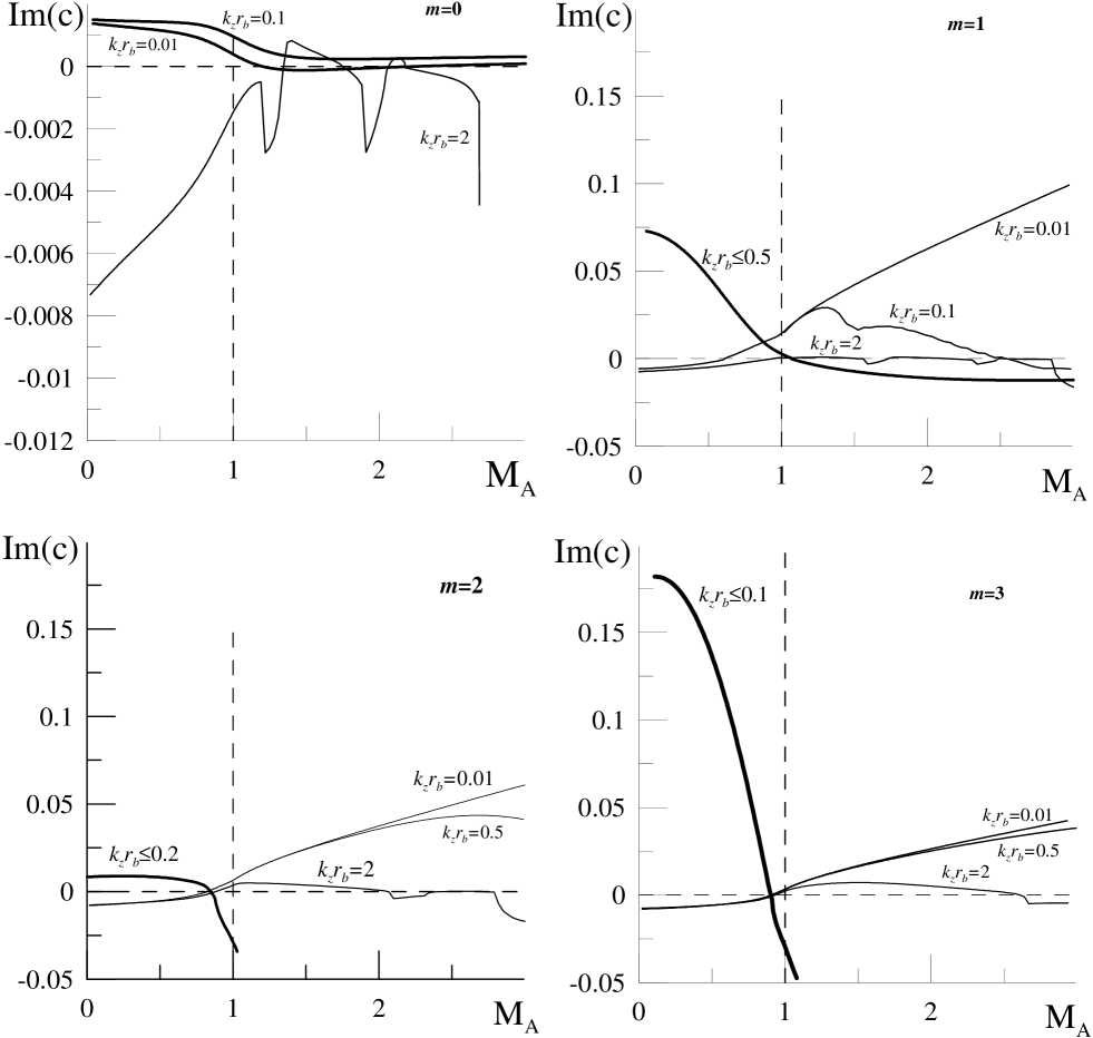
Figure 7: Mach number $M_{A}$ dependence of the increment of MHD oscillations of the cylindrical plasma jet for the first azimuthal harmonics $m=0,1,2,3$ and different magnitudes of parameter $k_{z}r_{b}$. The distributions of the increment for the oscillations with $k_{z}r_{b}=2$ (thin lines) defined by the local instability of the jet boundary are presented on all the panels. For the harmonics $m\neq 0$ the distributions are also presented of the increment of local instability for the oscillations with $k_{z}r_{b}<1$ (thin lines). Thick lines show the distributions of the increment of the ”global modes” of the plasma jet oscillations.

Let us try to understand qualitatively the nature and features of these oscillations by analyzing their spatial structure in fig.6b. First of all it should be noted that these oscillations have an almost homogeneous structure of the first derivative $d\zeta/dr\approx const=C_{I}$ in the plasma jet, whence we obtain $\zeta=C_{I}r$ (we suppose $\zeta(r\rightarrow 0)\rightarrow 0$). This means that the oscillations occupy the entire cross-section of the plasma jet and have a constant amplitude there. We will call such oscillations ”global modes” of the plasma jet. The dispersion equation for such modes can be obtained using the matching conditions (1cf) on the plasma jet boundary. For this purpose we will integrate equation (1cd) in the interval ($0,r_{b}$) using an approximate expression $\zeta=C_{I}r$ for $\zeta$:

$$\left.\frac{\rho_{0}\Omega^{2}}{k_{r}^{2}r}\frac{\partial r\zeta}{\partial r}\right|_{r=r_{b}-\varepsilon}=-\int_{0}^{r_{b}}\rho_{0}\Omega^{2}\zeta dr\approx-C_{I}\int_{0}^{r_{b}}\rho_{0}\Omega^{2}rdr$$

and substitute the resulting expression into the matching condition (1cf) assuming the region outside of the jet to be opaque. As a result we obtain the following dispersion equation

$$\int_{0}^{r_{b}}\rho_{0}\Omega^{2}rdr=\frac{\rho_{0II}\Omega_{II}^{2}r_{b}}{\sqrt{-k^{2}_{rII}(r_{b})}},$$

or, in the dimensionless form,

$$\int_{0}^{r_{b}}\left(\frac{c^{2}}{v_{A}^{2}(r)}-1\right)rdr=\frac{r_{b}\left[(c-M_{A})^{2}/\epsilon^{2}-1\right]}{b\sqrt{-k^{2}_{rII}(r_{b})}},$$ (1cal)

where

$$k^{2}_{rII}=k_{z}^{2}\left(\frac{(c-M_{A})^{4}/\epsilon^{4}}{(c-M_{A})^{2}(1+\beta^{*}_{II})/\/\epsilon^{2}-\beta^{*}_{II}}-1-\kappa_{m}^{2}\right),$$

$v_{A}(r)=A(r)/A_{I}$, $b=B_{0I}^{2}/B_{0II}^{2}$, $\epsilon=A_{II}/A_{I}\ll 1$, $\kappa_{m}=m/k_{z}r_{b}$.

Let us apply the perturbation theory to searching for a solution to (1cal), expanding $c$ into a (1cae)-like series with $\epsilon$ being the small parameter. In the zeroth order of the perturbation theory, we have $c_{0}=M_{A}$ as before. In the first order of the perturbation theory, we obtain an equation for $c_{1}$

$$\frac{c_{1}^{2}-1}{\sqrt{1+\kappa_{m}^{2}-c_{1}^{4}/[c_{1}^{2}(1+\beta^{*}_{II})-\beta^{*}_{II}})]}=\int_{0}^{r_{b}}\left(\frac{M_{A}^{2}}{v_{A}^{2}(r)}-1\right)rdr.$$ (1cam)

Let us consider two cases.

7.1 Case $m\neq 0$

When the parameter $k_{z}r_{b}$ is small enough ($\kappa_{m}\rightarrow\infty$, $k_{z}r_{b}\rightarrow 0$) we obtain the following approximate solution of (1cam):

$$c_{1}^{2}\approx bm\int_{0}^{1}\left(\frac{M_{A}^{2}}{v_{A}^{2}(x)}-1\right)xdx,$$

where $x=r/r_{b}$ and $b\gg 1$. It is easy to see from here that the unstable oscillations ($c_{1}^{2}<0$) exist only when the condition

$$\int_{0}^{r_{b}}\rho_{0}(r)\left(v_{0II}^{2}-A^{2}(r)\right)rdr<0,$$

holds, which also determines the magnitude of $M_{Ac}$. When $k_{z}r_{b}\rightarrow 0$ the magnitude of ${\rm Im}(c)$ does not depend on $k_{z}r_{b}$, which agrees completely with the numerical calculations in the previous Section.

7.2 Case $m=0$

If $|c_{1}|\gg 1$ (for example when $b\gg 1$, but $|\epsilon c_{1}|\ll c_{0}$) we have the following solution of (1cam)

$$c_{1}\approx\pm\frac{i}{\sqrt{1+\beta^{*}_{II}}}bk_{z}r_{b}\int_{0}^{1}\left(\frac{M_{A}^{2}}{v_{A}^{2}(x)}-1\right)xdx.$$

There is no limiting magnitude of $M_{Ac}$ for this solution, defining the region of existence for unstable oscillations, but there is a dependence on $k_{z}r_{b}$. This also agrees qualitatively with the above numerical calculations. Note that the solutions obtained in this way should only be regarded as an illustration of the qualitative behaviour of the global oscillation modes. The exact values of their increment obtained numerically may differ considerably from these simplified estimates.

8 Conclusion

Let us enumerate the main results of this work.

1. Qualitative analysis of the solution of (1cd), describing the MHD oscillations of a cylindrical plasma jet, has shown that its boundary is unstable in relation to the fast magnetosonic oscillations in the range of the flux parameters $1<M_{A}<M_{2}$ (where $M_{A}=v_{0II}/A_{I}$ is the Mach number found from the maximum Alfven speed, $M_{0}<M_{1}<1$; $M_{2}>1$ are the characteristic Mach numbers defined in Section 5 in the WKB approximation over the radial coordinate).

2. The boundary of the plasma jet also becomes unstable when $M_{A}$ approachs one of the eigenvalues $c_{0n}={\rm Re}((\omega/k_{z})_{n}/A_{I})$ defined by the dispersion equation for FMS and SMS oscillations in the resonator: $\tan(\psi(c_{0n})+\pi/4)=0$, $n=1,2,3...$, where $\psi$ is spatial oscillation phase from the turning point to the plasma jet boundary, $(\omega/k_{z})_{n}$ is the parallel phase velocity of the $n$-th harmonic of the oscillations. The ranges of $M_{A}$ where the unstable oscillations exist are located close to $c_{0n}$ - in the range $M_{A}>M_{2}>1$ for FMS waves, and $M_{0}<M_{A}<M_{1}<1$ for SMS-waves.

3. A numerical solution of the problem for a cylindrical plasma jet with a smooth boundary layer has shown that the range of $M_{A}$ values where the jet boundary is unstable corresponds qualitatively to those obtained in the WKB approximation for the jet with a sharp boundary. There are essential differences, however. Firstly, the absolute values of the increment of unstable oscillations for the jet with a smooth boundary layer are much smaller than those for the jet with a sharp boundary. This is explained by a smoothing of the boundary and by competition between the instability of the shear flow and the dissipation of the oscillation energy on the resonance surfaces for the Alfven and SMS waves. The number of unstable harmonics of the eigen-oscillations of magnetosonic resonators in the plasma jet is restricted by a few first harmonics. Secondly, the ranges of the $M_{A}$ values for unstable modes of the oscillations in the jet with a smooth boundary are considerably displaced relative to the location obtained for the jet with a sharp boundary.

4. It is shown that, in addition to local instability of the jet boundary, there exist also unstable ”global modes” of the plasma jet oscillations. Their amplitude is almost constant in the entire cross-section of the jet, while its instability increments are much larger than those for unstable oscillations of the jet boundary. The range of $M_{A}$ values for which the ”global modes” are unstable begins from $M_{A}=0$. The distribution of the increment of such oscillations differs substantially between the axisymmetric ($m=0$) and asymmetrical ($m\neq 0$) modes. Modes with $m\neq 0$ only become unstable for rather small magnitudes of the parallel wave number ($k_{z}r_{b}<(k_{z}r_{b})_{max}<1$), the region of their existence being restricted by the range $0<M_{A}<M_{Ac}$ (where $M_{Ac}$ is the limiting magnitude $M_{A}$ until which the ”global modes” remain unstable, different for each $m$). The distribution of the increment of such oscillations is almost the same for any oscillations with $k_{z}r_{b}<(k_{z}r_{b})_{max}$. Unstable axisymmetric ”global modes” are not limited in the $M_{A}$ value and their increment depends essentially on the magnitude of parameter $k_{z}r_{b}$.

References

References

• [1] McKenzie J F 1970 Planet. Space Sci., 18, 1
• [2] Kivelson M G, Pu Z-Y 1984 Planet. Space Sci., 32, 1335
• [3] Watson M 1981 Geophys. Astrophys. Fluid Dynamics, 16, 285-298
• [4] Rosenbluth M N and Longmire C L 1957 Annals of Physics, 1, 120-140
• [5] Lukiyanov 1975 Hot Plasma and Controlled Fusion (in Russian), (Nauka: Moskow), p. 407
• [6] Perkins W A and Post R F 1963 Physics of Fluids, 6, 1537-1558
• [7] Landau L D 1944 Akad. Nauk S.S.S.R., Compts Rendus (Doklady), 44, 139-142
• [8] Thorpe S A 1969 J. Fluid Mech., 36, 673-683
• [9] Miura A 1992 J. Geophys. Res., 97, 10655–10675
• [10] Fujita S, Glassmeier K H, Kamide K 1996 J. Geophys. Res., 101, 27317-27326
• [11] Leonovich A S and Kozlov D A 2009 Plasma Phys. Control. Fus., 51, 085007
• [12] Chen L and Hasegawa A 1974 Phys. Fluids, 17, 1399
• [13] Erdelyi R 2004 Astronomy and Geophysics, 45, 4.34
• [14] Azovsky Yu C, Guzhovsky I T, Pistryak V M 1967 in Investigations of a plasma clusters, (in Russian), (Naukova Dumka: Kiev), 56-65
• [15] Filippov B, Golub L, Koutchmy S 2009 Solar Phys. , 254, 259- 269
• [16] McKenzie J F 1970 J. Geophys. Res., 75, 5331-5339
• [17] Drazin P G and Howard L N 1966 Adv. Appl. Mech., 9, 1-89